Critically Reassessing Tropospheric Temperature Trends from Radiosondes Using
Realistic Validation Experiments
HOLLYA. TITCHNER, P. W. THORNE,ANDM. P. MCCARTHY Met Office Hadley Centre, Exeter, United Kingdom
S. F. B. TETT
School of Geosciences, University of Edinburgh, Edinburgh, United Kingdom
L. HAIMBERGER
Department of Meteorology and Geophysics, University of Vienna, Vienna, Austria
D. E. PARKER
Met Office Hadley Centre, Exeter, United Kingdom
(Manuscript received 8 January 2008, in final form 5 June 2008) ABSTRACT
Biases and uncertainties in large-scale radiosonde temperature trends in the troposphere are critically reassessed. Realistic validation experiments are performed on an automatic radiosonde homogenization system by applying it to climate model data with four distinct sets of simulated breakpoint profiles. Knowl-edge of the ‘‘truth’’ permits a critical assessment of the ability of the system to recover the large-scale trends and a reinterpretation of the results when applied to the real observations.
The homogenization system consistently reduces the bias in the daytime tropical, global, and Northern Hemisphere (NH) extratropical trends but underestimates the full magnitude of the bias. Southern Hemi-sphere (SH) extratropical and all nighttime trends were less well adjusted owing to the sparsity of stations. The ability to recover the trends is dependent on the underlying error structure, and the true trend does not necessarily lie within the range of estimates. The implications are that tropical tropospheric trends in the unadjusted daytime radiosonde observations, and in many current upper-air datasets, are biased cold, but the degree of this bias cannot be robustly quantified. Therefore, remaining biases in the radiosonde tem-perature record may account for the apparent tropical lapse rate discrepancy between radiosonde data and climate models. Furthermore, the authors find that the unadjusted global and NH extratropical tropospheric trends are biased cold in the daytime radiosonde observations.
Finally, observing system experiments show that, if the Global Climate Observing System (GCOS) Upper Air Network (GUAN) were to make climate quality observations adhering to the GCOS monitoring principles, then one would be able to constrain the uncertainties in trends at a more comprehensive set of stations. This reaffirms the importance of running GUAN under the GCOS monitoring principles.
1. Introduction
There has been much debate surrounding tropical tropospheric temperatures since the first attempt to create a satellite-based climate dataset (Spencer and
Christy 1990). Climate models predict amplification of the observed tropical warming trends at the surface (Santer et al. 2005; Karl et al. 2006), with maximum warming rates expected in the middle and upper tro-posphere. The observations are currently inadequately characterized to statistically robustly inform on this issue (Santer et al. 2008). The Remote Sensing Systems (RSS) (Mears and Wentz 2005), the University of Maryland (Vinnikov et al. 2006), and the National Environmental Satellite Data and Information Service (Zou et al. 2006) Corresponding author address:Holly Titchner, Met Office
Had-ley Centre, FitzRoy Road, Exeter, Devon EX1 3PB, United King-dom.
E-mail: [email protected] DOI: 10.1175/2008JCLI2419.1
Microwave Sounding Unit (MSU) datasets all yield trends that are more or less consistent with model predictions. So do some more recent radiosonde temperature data-sets (Sherwood et al. 2008a; Haimberger et al. 2008) and temperatures inferred from radiosonde winds (Allen and Sherwood 2008). However, other recently produced radiosonde datasets (Haimberger 2007; Thorne et al. 2005b; Free et al. 2005) and the University of Alabama in Huntsville (UAH) (Christy and Norris 2006) MSU dataset have all reported less warming aloft than ex-pected since 1979 (Karl et al. 2006). Here we aim to robustly reassess the uncertainty in the manually ho-mogenized Met Office Hadley Centre radiosonde tem-perature dataset (HadAT) (Thorne et al. 2005b), which should better inform where the truth lies.
There have been numerous changes to the global ra-diosonde observing network throughout the last few decades, many of which have been poorly documented. This has resulted in many sudden changes (inhomoge-neities or breakpoints) within the long-term time series. The challenge is to remove these breakpoints and re-cover the large-scale trends, which are small relative to both the natural variability and the magnitude of many of the identified breakpoints. However, our ability to do this is highly dependent on the decisions made dur-ing homogenization (Thorne et al. 2005a). The result-ing structural uncertainty is reflected in the different trend estimates produced by the existing datasets (Free and Seidel 2005; Karl et al. 2006).
McCarthy et al. (2008) developed an automated sys-tem, adapted from the manual HadAT dataset (Thorne et al. 2005b), that attempts to homogenize a radiosonde dataset using neighbor-based iterative breakpoint iden-tification and adjustment. The homogenization is con-trolled by a number of system parameters that can be set to different values, akin to making different meth-odological decisions during the dataset development. The system can be used to output a large ensemble of different dataset realizations. McCarthy et al. (2008) used a very simple validation ensemble and found that, when trends are systematically biased, many experi-ments did not fully recover the true large-scale trend.
In this study we develop four error (or breakpoint) models based on different, much more complex, as-sumptions in order to produce breakpoint profiles that could exist in the real world. This extends the idealized experiments performed by McCarthy et al. (2008). The four different error models are applied to homoge-neous third Hadley Centre Atmospheric Model (HadAM3) (Pope et al. 2000) climate simulation data from a run with prescribed historical sea surface tem-peratures and natural and anthropogenic forcings.
Tem-poral and spatial sampling characteristics of the daytime and nighttime observed radiosonde data are imposed on the model data. The resulting heterogeneous data are passed through the automatic homogenization system, and a population of 100 realizations is produced by varying the homogenization system parameters in a series of experiments. The only difference between each of the 100 experiments therefore relates to the homogeniza-tion method used. The same 100 experimental setups are used for each of the daytime and nighttime error model input datasets as well as the observations. Knowing the original model ‘‘truth’’ we can assess the ability of the system to recover the large-scale trends from heteroge-neous data. These validation experiments permit a criti-cal reappraisal of the trends produced when the system is applied to the real observations, enabling us to make inferences about the real world trends. We also run some observing system experiments using the error models in order to assess the impact of future possible changes to the radiosonde network and possible av-enues to improve our knowledge of historical data. Al-though our homogenization experiments are performed on levels between 850 and 30 hPa, we focus on the troposphere, particularly on the tropics. Our main aim is to assess whether the apparent tropical tropospheric lapse rate discrepancy, supported by many, but not all, currently available radiosonde datasets, could be due to uncertainty in the radiosonde records.
2. Input data
a. Radiosonde data
The radiosonde observations used within this study were derived from the raw daily data that were input into the Radiosonde Observation Correction Using Re-analyses (RAOBCORE) dataset (Haimberger 2007). This dataset is a merge of radiosonde ingest to the 40-yr European Centre for Medium-Range Weather Fore-casts (ECMWF) Re-Analysis (ERA-40) (Uppala et al. 2005) and the Integrated Global Radiosonde Archive (IGRA) (Durre et al. 2006), with preference given to ERA-40 ingest data. Data at 12 standard pressure lev-els (850, 700, 500, 400, 300, 250, 200, 150, 100, 70, 50, and 30 hPa) were used from 1958 to 2003.
were included, to limit the seasonality of polar day and night. We excluded Indian stations, which have previ-ously been found to be problematic (Thorne et al. 2005b; Lanzante et al. 2003; Parker et al. 1997). Sea-sonal anomalies were calculated relative to 1981–2000 climatology. This increased the coverage by 28 stations in the tropics (208S–208N) during the satellite era, which is the focus of this paper, compared with using 1966–95 climatology, as done by McCarthy et al. (2008) and Thorne et al. (2005b) to maximize the global cov-erage for the full period. The resulting daytime dataset contained a total of 586 (79 in the tropics) stations and the nighttime dataset contained 513 (29 in the tropics) stations (Fig. 1a).
We also use metadata documenting known changes of instruments and observing practices. These came from the IGRA dataset [Gaffen(1996) and subse-quent updates]. While these metadata provide valuable information regarding the timing of potential breaks, they are often incomplete. Around 70% of identified breakpoints in the HadAT (Thorne et al. 2005b) and RAOBCORE (Haimberger 2007) datasets had no known metadata events associated with them. Many of these breaks were large and very likely arose from un-recorded changes at the stations, rather than from false breakpoint identifications.
b. Simulated data
We perform validation experiments using simulated data from HadAM3 (Pope et al. 2000), forced with observed sea surface temperature and sea ice distribu-tions from the Hadley Centre Sea Ice and Sea Surface Temperature (HadISST) dataset (Rayner et al. 2003) and prescribed anthropogenic and natural external forcings (Tett et al. 2007). The advantage of using these data, instead of simply producing a randomly generated series, is that they contain a representation of real variations in the climate (such as ENSO) that may be expected to interact with the ability of any homogeni-zation system to identify and adjust for breaks.
The monthly model data were available at 10 of the 12 radiosonde observation pressure levels (all except 70 and 30 hPa) on a 2.58latitude by 3.758longitude grid. Data from the nearest grid box to each station were extracted. The data were subsampled twice, once using the daytime observation coverage and once using the nighttime coverage, to produce two datasets. Seasonal anomalies were created for each station relative to a 1981–2000 climatology. Random noise with a Gaussian distribution and standard deviation of half that of the model gridbox series was added to approximate sam-pling effects and to ensure that no two station series
arising from the same grid box would contain exactly the same data. The two resulting model datasets pro-vide homogeneous records with the same spatial and temporal sampling as the daytime and nighttime obser-vational datasets. We refer to these as control datasets.
3. Methods
a. Homogenization system
The homogenization system developed by McCarthy et al. (2008) uses an iterative neighbor-based break-point identification and adjustment technique similar to that employed in the development of the HadAT ra-diosonde dataset (Thorne et al. 2005b). Reference anomaly series are generated as weighted composites of neighboring stations, with weightings derived from temperature correlation coefficients calculated using ei-ther National Centers for Environmental Prediction (NCEP) (Kalnay et al. 1996) or ERA-40 (Uppala et al. 2005) reanalyses since 1979. A station minus neighbor difference series is then calculated, which is intended to remove the majority of the natural climatic variations and large-scale trends and emphasize nonclimatic change points. The success of this depends upon how well errors in the neighbor series cancel when averaged together.
The Kolomogorov–Smirnov (K–S) test (Press et al. 1992), a nonparametric statistical homogeneity test, is used to identify breakpoints in the station minus neigh-bors difference series. Pressure levels are considered in unison during the breakpoint identification, as the breakpoints are assumed to affect multiple (although not necessarily all) levels. Information regarding the sign of the potential breakpoints is not used at this stage. The statistical breakpoint test result series is combined with information based on the metadata. The metadata therefore provide additional evidence but are not usually crucial for the identification of a break-point. A critical threshold is used to assign breakpoints within this combined series. See Fig. 1 in McCarthy et al. (2008) for an example of this breakpoint identifica-tion method.
density of stations that do not have contemporaneous breaks. There are 14 tunable parameters within the sys-tem (appendix A of McCarthy et al. 2008), which affect the location and timing of the breakpoints identified and how the adjustments are calculated. For a more detailed description of the system, parameters, and limitations see section 3 of McCarthy et al. (2008).
Once the homogenization is completed, the anoma-lies are averaged onto a 58 latitude by 108 longitude grid, as in HadAT (Thorne et al. 2005b). They are then vertically weighted to replicate lower-tropospheric T2LT (Karl et al. 2006) temperature anomalies mea-sured by MSU and to allow dataset comparisons (see section 5). Static MSU weighting functions have been provided by the University of Alabama in Huntsville. Latitude bands are averaged and cos(lat) weighted to calculate global, tropical (208S–208N), Northern Hemi-sphere (NH) extratropical (208–708N), and Southern Hemisphere (SH) extratropical (208–708S) mean time series. Linear trends for the satellite era were estimated using the median of pairwise slopes method (Lanzante 1996) to minimize the effect of outliers. It is important to note that the true time series behavior is not neces-sarily linear and that alternative time series descriptors may be equally valid (Seidel and Lanzante 2004; Thorne et al. 2005b).
b. Derivation of error models
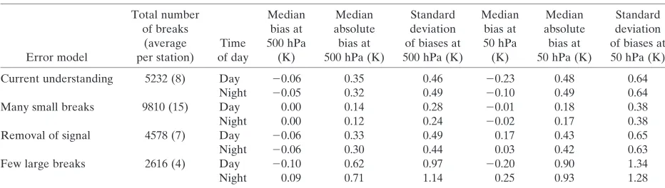
To rigorously test the homogenization system we ap-ply artificial breakpoint profiles to the daytime and nighttime control datasets from the climate model. The numbers, dates, and profiles of the breakpoints varied between four different error models (Table 1). Each error model was based on different assumptions regard-ing the size, distribution, etc., of the breakpoints (see appendix A for more details). They were applied at the same dates in the daytime and nighttime datasets,
al-though different breakpoint profiles were used for these two datasets. This is consistent with published results from radiosonde intercomparisons (Nash et al. 2005) that yield different error structures for day and night.
Figure 2 shows the distribution of daytime break-point sizes for each error model at 50 hPa. A positive (negative) breakpoint is said to occur when there is an increase (decrease) in the mean of the later part time series compared to the mean in the earlier part of the time series. Although we will later concentrate on the troposphere, we chose to illustrate the break-points applied at 50 hPa because they are larger than in the troposphere, as is also strongly believed to be the case in the observations (Karl et al. 2006), and hence the systematic biases can be more easily seen. The main features of each error model are summa-rized below.
d Current understanding. This error model is our
cur-rent understanding based upon existing literature of the breakpoints that afflict the observed temperature record in the radiosonde network. The breakpoints above 500 hPa have a negative mean (Table 1, Fig. 2a) in order to produce a cooling bias in the long-term trends. Breakpoints in the daytime dataset have an additional negative offset, as McCarthy et al. (2008) and Sherwood et al. (2005) found in observa-tions.
d Many small breakpoints. Although this error model
does contain some large breakpoints, it contains a large number of smaller ones (Table 1, Fig. 2b). These small breakpoints have only a very small sys-tematic bias.
d Removal of signal. Breakpoints at or below 150 hPa
have a negative offset and those above have a posi-tive offset (Table 1, Fig. 2c) similar in magnitude to the temperature trend in the model. The net result is
TABLE1. The total number of breakpoints applied within each error model and a summary of the breakpoint sizes applied at
500 hPa and 50 hPa.
Error model
Total number of breaks
(average per station)
Time of day
Median bias at 500 hPa
(K)
Median absolute bias at 500 hPa (K)
Standard deviation of biases at 500 hPa (K)
Median bias at 50 hPa (K)
Median absolute bias at 50 hPa (K)
Standard deviation of biases at 50 hPa (K)
Current understanding 5232 (8) Day 20.06 0.35 0.46 20.23 0.48 0.64
Night 20.05 0.32 0.49 20.10 0.49 0.64
Many small breaks 9810 (15) Day 0.00 0.14 0.28 20.01 0.18 0.38
Night 0.00 0.12 0.24 20.02 0.17 0.38
Removal of signal 4578 (7) Day 20.06 0.33 0.49 0.17 0.43 0.65
Night 20.06 0.30 0.44 0.03 0.42 0.63
Few large breaks 2616 (4) Day 20.10 0.62 0.97 20.20 0.90 1.34
to remove most of the underlying climate change sig-nal.
d Few large breakpoints. This error model contains
fewer breakpoints than the other error models but with a larger standard deviation, resulting in a higher proportion of large breakpoints (Table 1, Fig. 2d).
Except in the case of thecurrent understandingerror model, where daytime breakpoints are given a negative offset in comparison to nighttime breakpoints, the dif-ferences between the daytime and nighttime error structures only arise from random differences in the generation of the breakpoint profiles. The differences in median biases (Table 1) are more evident at 50 hPa where the sample is smaller, as in the real observations. The main difference between the daytime and night-time datasets is that nightnight-time has a much poorer spa-tial coverage, particularly outside the NH extratropics (Fig. 1a).
The error models can be used to assess the skill of a homogenization method on data containing different error structures, as the breakpoint locations and
mag-nitudes, and climate change signal are known. They are also more complex than idealized test cases employed in many earlier tests of homogenization methods (e.g., McCarthy et al. 2008; Haimberger 2007; Sherwood et al. 2008a) and allow for a more comprehensive under-standing of the trend uncertainties. The four error mod-els used within this study were deliberately designed to be as different as possible so that the system is not tuned toward a given set of assumptions. They span a range of possible error structures, all of which may con-tain at least some characteristics (e.g., phasing, bias, magnitude, clustering) that exist within the true obser-vations.
c. Homogenization ensembles
We perform an ensemble of 100 homogenization ex-periments on each dataset by randomly varying the 14 tunable system parameters listed in appendix B. Each homogenized output represents a different set of meth-odological choices and can be used to investigate un-certainty in trends resulting from the homogenization
FIG. 2. Breakpoint distributions at 50 hPa for each daytime error model. A positive (negative) breakpoint is said
to occur when there is an increase (decrease) in the mean of the later part time series compared to the mean of the earlier part of the time series. The number of breakpoints and the shape of the distributions vary between error models. The distribution also varies with height, with lower levels showing a similar shape but with a smaller
absolute spread. The zero line is marked by the vertical dashed line, which highlights the negative bias in thecurrent
(McCarthy et al. 2008). The same 100 random param-eter configurations were used for each ensemble so that the only difference between each ensemble was the in-put dataset. The variations within a given ensemble are therefore entirely due to differences in the tuning of the homogenization method. Ensembles were created for each of the daytime and nighttime datasets: the observations, the control datasets, and the four error models. Ensembles using the original control datasets were produced simply to assess the impact of homog-enizing breakpoint-free data. It is important to as-certain whether the system significantly alters these data as that would clearly be an undesirable character-istic.
d. Homogenization skill rankings
As well as assessing the absolute values of the trends produced from the homogenization system for error model ensembles, we also assess the relative skill within ensembles by ranking local error recovery and large-scale fidelity (see below). By comparing the rankings between each error model we can see whether particu-lar experiments consistently do well (or poorly) and, therefore, determine how dependent the homogeniza-tion skill is on the underlying error structure. If there is little dependence, then we will be able to unambigu-ously tune our system toward a more reliable set of experiments and exclude the experiments we know to be ineffective. The two approaches we use to rank the experiments are summarized below.
d Local skill. Provides a measure of how well each
ex-periment identifies breakpoint locations and magni-tude. We compare the root-mean-square difference (RMSD) between the known error model time series and the control series for each station and level with the RMSD between the homogenized series and the control series. The values are summed over all stations and levels to yield a single value for each experiment within a given ensemble. The experiment values are then ranked between 1 and 100 (1 indi-cating closest agreement to the known error struc-ture). A high local skill score therefore indicates an experiment that provides accurate local observations relative to the other experiments within the given ensemble.
d Trend recovery. Provides a measure of how
success-ful each experiment is at capturing the ‘‘true’’ mean T2LT trend in the satellite era for a given large-scale region (global, tropical, NH extratropical, or SH ex-tratropical). The experiments are ranked between 1 and 100 (1 indicating the best) based on how closely they estimate the trend in the unbiased control series.
4. Error model results
a. Ranking results
Using the method outlined in section 3d, Fig. 3 com-pares the local skill rankings for themany small breaks andremoval of signaldaytime ensembles. The cluster-ing around the 1:1 line and the high correlation be-tween the rankings show that there is good agreement as to how the homogenization system performs on these two error models. The correlations between the other error models for both daytime and nighttime were also found to be high (Table 2). This is encourag-ing and indicates that the ability of the system to reduce RMSD is not very dependent on the underlying error structure. A total of 35 (32) experiments consistently rank in the top half for the daytime (nighttime) error model ensembles. Assuming that the error models are uncorrelated, if the system showed no skill, it would effectively become a random number generator. Under this assumption the degree of agreement actually found is considerably more than would be expected from a set of four random number populations (10030.5456). We also produced separate rankings for the tropo-sphere only and found very similar results (not shown). The absolute RMSD values reveal that nearly all
ex-FIG. 3. A comparison of the local skill rankings for themany
periments improve local skill relative to making no ad-justments (Table 3). Any breakpoints identified and adjusted for in the control experiments are false, and so are detrimental to the local skill and trend. However, the RMSD values for the control ensembles were found to be an order of magnitude smaller than the RMSD values for error models. The benefit (in terms of RMSD, i.e., the accuracy of local observations) of ad-justing data in the presence of biases is therefore much greater than the cost if no errors exist.
Figure 4 compares the tropical trend recovery rank-ings for the current understanding and many small breaks daytime ensembles. The correlations (Table 4) show that these rankings are less consistent than the local skill rankings. Therefore, skill in recovering large-scale trends depends on the underlying error structure. Also, an experiment that is relatively skillful at mini-mizing RMSD error is not necessarily skillful at recov-ering the large-scale trends (Sherwood et al. 2008b). However, there are still 17 experiments that consistently rank in the top half for all daytime error models, which is more than expected by chance. A total of 12 daytime experiments rank in the top half for both tropical trend recovery and local skill (only 10030.58,1 is expected by chance), 7 of which also rank in the top half for the global and NH extratropical trend recovery. We refer to these seven experiments as our ‘‘top’’ experiments throughout the rest of this paper. SH extratropical re-sults are ignored as there is poor agreement between the error model trend rankings in this region (only three experiments consistently rank in the top half using these rankings alone) owing to the sparsity of SH
extra-tropical stations (Fig. 1a). Although the extra-tropical stations are equally sparse, their neighbor correlation regions are larger, so the homogenization performs better there, as reflected in the better agreement between error model rankings. We only consider the best performing experiments for the daytime data as there is extremely poor agreement between the nighttime error models: only 7 consistently rank in the top half using the tropical trend recovery rankings alone, again owing to data sparsity.
An examination of the parameter settings for the ‘‘top’’ experiments did reveal that they all used an ‘‘adaptive’’ adjustment method (i.e., all adjustments are recalculated during every iteration unlike the ‘‘non-adaptive’’ adjustment method; see appendix A and sec-tion 3 of McCarthy et al. 2008 for more details). No other parameter settings stand out as being optimal. However, 100 experiments is not a large enough sample
TABLE2. Rank correlations between local error recovery skill for each error model based on the day (lower-left-hand triangle) and
night (italic, upper-right-hand triangle) RMSD. Correlations between the day and night RMSD rankings for each individual error model are given on the diagonal (bold).
Current understanding Many small breaks Removal of signal Few large breaks
Current understanding 0.80 0.89 0.95 0.66
Many small breaks 0.68 0.97 0.86 0.48
Removal of signal 0.85 0.90 0.98 0.78
Few large breaks 0.84 0.90 0.97 0.80
TABLE3. The number of homogenized series that have a lower
RMSD or trend error than each unadjusted error model for day and night.
Error model
RMSD Trend
Day Night Day Night
Current understanding 98 98 88 21
Many small breaks 94 84 70 2
Removal of signal 100 100 93 38
Few large breaks 100 100 98 94
FIG. 4. As in Fig. 3 but using the tropical T2LT satellite-era
trend recovery rankings for thecurrent understandingandmany
with purely random parameter setting choices to thor-oughly investigate the effect of parameter values, as there are too many possible settings and many are likely to interact nonlinearly. A more detailed study with a larger number of experiments would be required to achieve this and is not the purpose of the current study.
b. Absolute trend results
We now consider the tropical T2LT satellite-era trend results from the daytime error model ensembles (Fig. 5a). By comparing the ensembles with the original control trend we can infer how well the system is likely to recover the true trend in the real observations. It can be seen that the spread in the daytime ensembles en-compasses the original (control) trend for all error models except for theremoval of signalcase. Although
the median trends underestimate the original trend, in all cases they reduce the trend bias. This is also re-flected in the daytime results for trend error in Table 3, which indicates that most experiments improve the tropical trend recovery in comparison to each unad-justed error model. The underestimation of the bias is partly due to the known inclusion of poor homogeni-zation experiments that are very conservative in the detection and adjustment of breakpoints and result in little or no change in trend compared to the unadjusted data. The trend in the unadjusted data does lie outside of or near the edge of the interquartile range for all error models. The medians of the top experiments are better at estimating the magnitude of the trend bias compared to the median of all experiments, and the original trend is almost recovered for the few large breakserror model, which is a priori the most tractable.
TABLE4. Rank correlations as in Table 2 except using the tropical T2LT trend recovery skill.
Current understanding Many small breaks Removal of signal Few large breaks
Current understanding 0.02 20.04 0.06 0.11
Many small breaks 0.25 0.12 0.25 20.04
Removal of signal 0.38 0.53 0.14 20.12
Few large breaks 0.33 0.14 0.54 0.25
FIG. 5. Tropical (a) daytime and (b) nighttime T2LT equivalent trends for the satellite period for
We infer that a median trend from a daytime ensemble is likely to correctly capture the sign of the trend bias, but is likely to underestimate the adjustment required (see also McCarthy et al. 2008). We can therefore infer the sign of the trend bias and place a strong lower limit on its magnitude from the median of the full ensemble. It is also likely that the true trend bias will be at least as large as the median of the top performing experiments, and possibly larger.
The nighttime tropical trend results are less encour-aging, which is reflected in the larger spread of solu-tions (Fig. 5b). Thus, there is a larger dependence on the error structure. Adjusted trends from all error mod-els except removal of signal do manage to encompass the original trend, but in many experiments there is a tendency for the adjustment to move the trend further from the truth. The bias in the median trend for all cases, exceptfew large breaks(recall this is a priori the most tractable), is similar to or worse than the trend in the unadjusted data. These results are also seen in Table 3 and must be due to the data coverage, which we recall is much poorer than for the daytime data (Fig. 1a). We therefore have very little confidence that re-sults from our system for the nighttime data in the trop-ics can provide a robust indication of the sign or mag-nitude of the systematic bias in the data.
Any breakpoints identified in the control experi-ments are false. In some control experiexperi-ments this erro-neously shifted the tropical T2LT trends up to 0.1 K decade21away from the already homogenous trends in
the daytime data, and up to 0.2 K decade21away in the nighttime data. This highlights the risk of relying upon a single homogenization method for trend estimation. However, 96 (86) daytime (nighttime) experiments shifted the trends by less than 0.05 K, and the median trends changed by less than 3% from the original con-trol trends. This suggests that false breakpoint detec-tion is not likely to be the major failing of a majority of the homogenization members. Further analysis of the error model ensembles (not shown) supports this and revealed that the underestimation of the trend bias in the majority of experiments occurred mainly as a result of missed breakpoints or incorrect adjustments, and not from falsely identified breakpoints.
The global tropospheric results are similar to those for the tropics, although the spread in the trend esti-mates tends to be smaller (Figs. 6a and 7a). The same applies to other subregions (Figs. 6b,c and 7b,c), al-though the SH extratropical trends for the daytime cur-rent understandingerror model (which are unbiased in the raw data) are shifted away from the truth, probably owing to sparsity of data. The NH extratropical
night-time data perform better than for the tropics and other subregions, as the median trend captures the right sign of the trend bias for all error models (albeit the median trend shifts very little for two of the error models). This is likely due to higher station density, better station management, and better quality metadata—all of which are important for the homogenization methodology.
5. Observation results
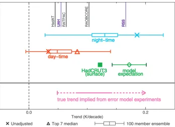
Figure 8 shows the tropical T2LT satellite-era trends for the adjusted observations produced from the same 100 experimental setups as those used for the error model ensembles. The unadjusted daytime trend is bi-ased cold relative to the climate model expectation of 0.14–0.20 K decade21based upon amplification of
sur-face trends (Santer et al. 2005). The median trend from the daytime ensemble shifts the trend closer, but the full spread,20.01–0.14 K decade21, does not quite en-compass the range of model estimates. The top experi-ments shift the median trend closer to the range based upon model expectation. The unadjusted daytime trend lies on the edge of the interquartile range, 0.03–0.07 K decade21. This is a relatively large spread compared to the daytime control ensemble, for example, which shifts the median trend very little.
The unadjusted nighttime trend, 0.19 K decade21, lies within the range of model expectation, although the median trend from the adjusted ensemble, 0.13 K de-cade21, is out of this range. The very large spread of the
adjusted trends, 0.03–0.23 K decade21, even
encom-passes the raw daytime trend.
We can make inferences about these real world trends using the results from the model-based experi-ments, although we are unable to calculate exact prob-abilities. The pink bar in Fig. 8 represents the true trend implied from the findings. However, we must caveat that the results are based on four out of an infinite number of possible error structures (see section 7). The following statements can be made about the tropical tropospheric trends:
d The trend in the raw daytime observations (0.03 K
decade21) is very likely biased cold (consistent with
McCarthy et al. 2008, Randel and Wu 2006, and Sher-wood et al. 2005), but we cannot comprehensively quantify the magnitude of the bias and its uncer-tainty.
d Our findings suggests that the true tropical trend is
d The tropical trends from many current datasets,
in-cluding HadAT (0.05 K decade21), are likely to be
biased cold.
d The true tropical trend may be warmer than the
range estimated from the daytime ensemble. There-fore remaining biases may still account for the appar-ent tropical lapse rate discrepancy between the ob-servations and climate models.
We now consider the T2LT satellite-era trends for the other large-scale regions (Fig. 9). The median en-semble trends indicate that the unadjusted daytime trends are biased cold globally and in the NH extra-tropics. In both cases the unadjusted trends also lie outside the interquartile range. We note that the me-dian trends from the global nighttime ensembles are only able to capture the correct sign of the bias for two
FIG. 6. As in Fig. 5 but for the (a) global, (b) NH extratropical, and (c) SH extratropical daytime
of the error models (Fig. 7a). However, in the other cases the median trend is shifted very little and the unadjusted trend falls well within the narrow interquar-tile range. The unadjusted trend from the night obser-vations (Fig. 9a), however, falls above the upper quar-tile. There is, therefore, some evidence for a warm glob-al nighttime bias, glob-although this is not robust. The median nighttime trend for the NH extra tropics does
capture the correct sign of the bias for all error models, even though the unadjusted trend sometimes lies within the interquartile range (Fig. 7b). Therefore Fig. 9b hints at a cold bias in the observed NH nighttime trends, although again this is not a robust result particularly as the unadjusted trend lies within a narrow interquartile range. Given the poor results from the validation ex-periments in the SH extratropics, we can say very little
FIG. 7. As in Fig. 5 but for the (a) global, (b) NH extratropical, and (c) SH extratropical
about the SH extratropical daytime and nighttime trends. The homogenization system therefore has little or no skill in this region.
We can only make the following inferences regarding Fig. 9 using the results from the validation experiments that are shown in Fig. 7:
d The unadjusted global daytime trend is very likely
biased cold, but we cannot comprehensively quantify the magnitude of the bias and its uncertainty.
d Our findings suggest that the true global trend is not
only warmer than the median trend from the daytime ensemble (0.11 K decade21), but also warmer than the median trend from the top experiments (0.12 K decade21).
d The unadjusted NH extratropical daytime trend is
very likely biased cold, but we cannot
comprehen-sively quantify the magnitude of the bias and its un-certainty.
d Our findings suggest that the true NH extratropical
trend is not only warmer than the median trend pro-duced from the daytime ensemble (0.27 K decade21),
but also warmer than the median trend from the top experiments (0.28 K decade21).
6. Assessing the value of the GUAN network
The error models can also be used to understand the effects of systematic changes to either the method em-ployed or the data used. The latter can guide us on future possible changes to radiosonde network. We perform two additional sets of experiments using the error models to assess the value of the Global Climate
FIG. 8. Tropical T2LT MSU equivalent trends for the satellite period. The red (daytime) and blue
Observing System (GCOS) Upper Air Network (GUAN). This is a small network of stations with a worldwide coverage sufficient for the detection of global-mean trends (McCarthy 2008).
a. Obtaining perfect metadata for GUAN stations
First, we assess the impact of accurately recording known instrumental or observational changes for the GUAN stations. We subsampled the GUAN stations (Fig. 1b) in the daytime (giving a total of 123 stations) and nighttime (giving a total of 77 stations) error model datasets and passed them through the system with no metadata. We then used the same data but this time with perfect metadata containing the correct timings of all breakpoints. The system was forced to apply adjust-ments at these breakpoint timings, although in some cases where breakpoints were close together only one adjustment may have been applied (see section 3 of McCarthy et al. 2008 for more details). We did this using the seven top experimental setups on the daytime and nighttime datasets for each error model.
High quality metadata do not have a beneficial im-pact on the T2LT tropical trends compared to using no metadata at all (Fig. 10). The median trend of each daytime ensemble changes very little. At night, perfor-mance with metadata is worse in two ensembles. This
may seem surprising given that the system is given per-fect knowledge of breakpoint locations, but there is still a requirement for the system to provide accurate ad-justments, which is particularly a challenge when only a few bad quality neighbors are used. It is likely that the GUAN nighttime coverage (Fig. 1b) is too sparse to create a sufficiently homogeneous neighbor composite series when only GUAN stations are used. It has al-ready been seen in section 4b that the poor coverage in the nighttime data inhibits the ability of our system to recover the large-scale trends even when the full net-work is used (albeit incomplete metadata were used). Sparsity of the GUAN nighttime stations may also cause more of a problem when given perfect metadata because the system is being forced to adjust all break-points, including the very small ones, in the early itera-tions because knowledge of metadata in these experi-ments all but guarantees breakpoint identification. b. Non-GUAN stations using perfect GUAN
stations as neighbors
We now investigate the impact of using a high quality set of GUAN stations (Fig. 1b) for homogenizing the rest of the network (Fig. 1c). This assesses the potential benefits of maintaining the GUAN network according to the GCOS climate monitoring principles. First, we
FIG. 9. (a) Global, (b) NH extratropical, and (c) SH extratropical observed T2LT equivalent
used the biased GUAN stations within each given error model to create the neighbor composite series, and then we used the perfect breakpoint-free GUAN sta-tions from the original control dataset. Again we used the seven top experimental setups for each of the day-time and nightday-time error model datasets.
The system is always better at capturing the true con-trol trend in tropical T2LT when the perfect GUAN stations are used as neighbors (Fig. 11). The improve-ments in theremoval of signalensembles are particu-larly noticeable, which is encouraging as this error model was the hardest to homogenize in the previous experiments (section 4b), though only seven experi-ments were used here. These results indicate a high quality reference series is important for trend recovery, and this may be a problem when a biased sparse net-work is used. If we could gain a high quality GUAN or similar-sized network, then it is very likely we would be able to adequately constrain the uncertainties in the trends for the rest of the global network.
7. Conclusions and discussion
The main aim of this study was to assess whether the tropical tropospheric lapse rate discrepancy between
climate models and some radiosonde datasets could conceivably be accounted for by uncertainty in the ra-diosonde records. To assess this uncertainty we devel-oped four substantially different error models. These error models contained artificial breakpoint profiles based on different assumptions about the underlying error structure. They were applied to HadAM3 climate model data, which were subsampled to the daytime and nighttime observations. These biased data were ad-justed using the automatic radiosonde homogenization system developed by McCarthy et al. (2008). We then assessed the ability of the system to recover the original large-scale trends, enabling us to make inferences about the biases and uncertainties in the real world observations.
The homogenization system produces a number of different realizations based on different methodological assumptions. A 100-member ensemble was created us-ing each daytime and nighttime error model dataset, as well as the observations. Changing the parameter set-tings influenced the breakpoints identified and the ad-justments calculated during the homogenization. This in turn affected the large-scale trends produced from each adjusted dataset.
Our prior knowledge of the original model trends
FIG. 10. Error model tropical T2LT trends using GUAN stations only for the (a) daytime and (b)
and the breakpoints within each error model enabled us to assess the homogenization skill of the system. Most experiments exhibited skill on a local observation basis relative to undertaking no homogenization at all. It was found that the performance of each member was fairly independent of the underlying error struc-ture when ranked according to this local skill, but more dependent when ranked according to the large-scale tropospheric trend recovery skill (also see Sherwood et al. 2008b).
Our results indicate that the bias in the daytime tropical tropospheric trends was underestimated by the majority of error models experiments. One of the four daytime error model ensembles (the removal of signal ensemble) was unable to capture the original model trend at all. We are therefore unable to guarantee that the spread in daytime observation ensemble encom-passes the real world trend. The change in the sign of the trend bias between the troposphere and strato-sphere is unlikely to have caused the poor performance using theremoval of signalerror model, as the system’s breakpoint identification and adjustment methodology should not be affected by such a change (see section 3a and McCarthy et al. 2008 for methodology details). However, a close examination of theremoval of signal error model revealed that it contained randomly gen-erated clustering of breakpoints at some times
through-out the series. This could cause problems during the homogenization and inhibit the system’s ability to re-cover the large-scale trends. It is possible that such clus-tering may occur in the real world observations. The cause could also be more complex still and relate to regional clustering and cancellation of errors, for ex-ample. The bottom line is that we have no unimpeach-able basis on which to reject at least some aspects of each error model being prevalent in the poorly under-stood real world raw data.
However, the bias in each unadjusted error model trend was correctly reduced to some extent both in the median ensemble member trend and even more so in an identified set of optimal experimental setups. We are therefore confident that the system correctly iden-tifies a cooling bias in the daytime observations, al-though we cannot robustly estimate the magnitude of the bias. Our analysis provides evidence that a lower bound of 0.08 K decade21 can be placed on our real world tropical T2LT trend uncertainty estimate, but does not provide an upper bound. This lower bound indicates that many current upper-air datasets, such as HadAT, are biased cold. Unfortunately, the tropical nighttime observation ensemble results are unable to provide an upper or lower bound, as many of the error model experiments were unable to reduce the night-time trend bias owing to the sparsity of data. Hence,
FIG. 11. As in Fig. 10 except using non-GUAN stations homogenized with error model biased
our analysis using realistic validation experiments is un-able to discount or confirm the presence of a tropical tropospheric lapse rate discrepancy between the radio-sonde observations and climate model expectations.
The daytime observations indicate that the unad-justed NH extratropical and global daytime trends are biased cold, although again we are unable to quantify the magnitude of these biases. There is some evidence that the unadjusted nighttime NH extratropical and global trends contain a cold and warm bias respectively, but this is not a robust result. Additional experiments would be required to investigate these biases further. The homogenization system performed particularly poorly in the SH extra tropics for some error models in both daytime and nighttime (likely owing to data spar-sity), therefore it has little or no skill in this region and we have no confidence in the observational results.
The results from the error models, and hence the implications for our current understanding, depend on a number of factors. There are an infinite number of error structures that could be created by further varying the different assumptions. There are a large number of assumptions that we have not varied, such as the data used to create our control dataset. The effect of using a particular set of randomly generated breakpoints for each error model has also not been properly investi-gated (although this has been varied to some extent between the different error models). Although there is uncertainty in our results related to these influences, the four error models used within this work spanned a sufficiently large range to provide useful results regard-ing the performance of the homogenization system and the true observational trends.
Results are also dependent on the actual homogeni-zation system being applied, therefore we will make our error model data freely available online at http://www. hadobs.org/ and encourage others to use them to criti-cally reassess their systems also. The range of trend estimates produced from each ensemble highlights the risk of relying upon a single homogenization method for trend estimation, particularly when there is no or little knowledge of optimal parameter settings or meth-odological choices. We therefore believe that much would be gained from a coordinated comparison of in-dependent radiosonde homogenization methods, par-ticularly if realistic validation experiments are per-formed. The error model data have proven useful al-ready in examining the new dataset produced by Sherwood et al. (2008a).
Sparsity of the network is likely to be accountable for the poor performance in some ensembles, particularly when compared to the ensembles that used a more comprehensive network, although the bias was
consis-tently underestimated even in these cases. One expla-nation may be that the system is unable to construct a sufficiently high quality neighbor reference series. The ability of the system to recover the trends in some or all ensembles may be improved if alternative methodologi-cal decisions are made in addition to those already tested. We are therefore undertaking further experi-ments on the error models by adding additional flex-ibility to the system to try to ascertain whether we can better constrain our trend estimates. These include re-moval of data around assigned breakpoints in the neighbor series, an assessment of sensitivity to the time interval of the input data, and use of different break-point statistical identification tests.
This study has not only given us a better understand-ing of the trend uncertainties, but it also allowed us to investigate the impacts of possible targeted changes to the radiosonde network. A number of further valida-tion experiments indicated that perfect metadata were unable to constrain the tropical tropospheric trend un-certainties using only GUAN stations. Results were much more encouraging when a GUAN network con-sisting of perfect station records was used as a reference series to homogenize the rest of the available stations. We therefore recommend that the GUAN network is maintained to a high standard, including adherence to the GCOS monitoring principles (GCOS 2004) so that we can have a better understanding of future trends in the free atmosphere.
Acknowledgments. Thanks to Steven Sherwood for comments on an earlier draft. Met Office Hadley Cen-tre authors (and Simon Tett during his time at the Met Office Hadley Centre) were supported by the Joint De-fra and MoD Integrated Climate Programme—GA01101, CBC/2B/0417_Annex C5. The work of Leo Haim-berger was supported by Contract P18120-N10 of the Austrian Fonds zur Fo¨rderung der wissenschaftlichen Forschung (FWF).
APPENDIX A
Error Model Assumptions
nighttime series under the assumption that discontinu-ities will occur at both times with any change in prac-tice. However, breakpoint profiles applied differed be-tween day and night. There is strong quantitative evi-dence for such behavior to be associated with radiosonde changes—at least through the series of WMO intercomparison projects (Nash et al. 2005 and references therein). Differences between the daytime and nighttime series within each individual error model therefore relate to these differing assumptions as to average day and night error structures as well as to coverage differences and to random differences in the breakpoint magnitudes.
The metadata record containing known breakpoints in the real world (Gaffen 1996, and subsequent up-dates) was used to assign some breakpoint locations within each error model. In some of these cases the same breakpoint profiles were applied to all break-points associated with a particular class of change. For example all changes from Vaisala RS80 to Vaisala RS90 had identical day breakpoints and identical night breakpoints applied.
Extra breakpoints were chosen by randomly select-ing stations and dates until the chosen total number of breakpoints was reached. In some error models a pro-portion of these extra breakpoints were assigned at the same date to all stations within the same country as a randomly selected station. In this case common
day-time breakpoint profiles and common nightday-time break-point profiles were applied to all stations within the country.
Vertically correlated breakpoint sizes were derived in order to create each breakpoint profile:
breakz5ð0:93breakz1Þ1nðmz;sÞ; ðA1Þ where breakzis the breakpoint size at a given pressure levelz(numbered 1 to 10, increasing height from 850 to 50 hPa), andnis an offset derived from a random dis-tribution with meanmz(at levelz) and standard
devia-tions. Here breakZ2150 forz51 (i.e., at 850 hPa);
mz andswere varied between each error model, and sometimes between different breakpoint profiles within an individual error model. Once each breakpoint pro-file was generated it was added to the daytime/night-time control series (section 2b) at and before the break-point date.
Table A1 summarizes the different assumptions made during the derivation of the error models and includes the values used in Eq. (A1). See Table 1 for a summary of the resulting set of breakpoints applied to each error model.
APPENDIX B
System Parameter Settings
The automated homogenization system contains a number of parameters that affect various components
TABLEB1. Possible settings for system parameters used in the ensemble experiments. Refer to McCarthy et al. (2008) for more
information.
Parameter name Description Possible settings
Neighbor weighting coefficients
Weighting coefficients for possible neighbor stations derived from reanalysis fields
NCEP or ERA-40
Country/metadata Excludes any neighbor stations within the same country/with similar
metadata records as the target station
Either both on or both off
K–S window width Number of seasons used for the K–S test used to assign breakpoints 8–20 seasons
Metadata weighting Weighting given to metadata events during the breakpoint identification
procedure (05no weight, 15breakpoint at every metadata event)
0.–1.
Metadata_function Shape of inversion in the metadata statistic series at known events Exponential or step
Vary metadata background
Alters the background value of the metadata probability series for each station based on the number of metadata events (i.e., penalizes stations with poor metadata records)
On or off
Range Minimum number of seasons required between each breakpoint 6–20 seasons
Critical value Initial critical threshold used to identify breakpoints in the first iteration 0.005, 0.02, or 0.05
Max iteration Number of iterations performed 3, 6, or 9
Iteration step Increment that the critical value is increased by with each iteration 0.005, 0.01, or 0.02
Adjustment method Adjustment method used. Adaptive recalculates all adjustments at each
iteration. Semiadaptive recalculates only if the breakpoint is found again at a later iteration. Nonadaptive calculates adjustment only when the breakpoint is first found
Adaptive or nonadaptive
Adjustment_period Number of seasons either side of each breakpoint used to calculate an
adjustment factor
5–20 or 40–55 seasons
Adjustment_threshold Thresholds for determining whether an adjustment should be applied or
not based on a points scoring system (appendix B; McCarthy et al. 2008)
of the homogenization process. These parameters are outlined in appendix A of McCarthy et al. (2008). Table B1 gives the range of settings used for each of the pa-rameters in the 100 experiments used within this study. For each of the 100 experiments the parameter values were randomly selected using a random number gen-erator on each range of settings.
REFERENCES
Allen, R. J., and S. C. Sherwood, 2008: Warming maximum in the
tropical upper troposphere deduced from thermal winds.
Na-ture Geosci.,1,399–403, doi:10.1038/ngeo208.
Brohan, P., J. J. Kennedy, I. Harris, S. F. B. Tett, and P. D. Jones, 2006: Uncertainty estimates in regional and global observed
temperature changes: A new data set from 1850.J. Geophys.
Res.,111,D12106, doi:10.1029/2005JD006548.
Christy, J. R., and W. B. Norris, 2004: What may we conclude
about global tropospheric temperature trends?Geophys. Res.
Lett.,31,L06211, doi:10.1029/2003GL019361.
——, and ——, 2006: Satellite and VIZ–radiosonde
intercompari-sons for diagnosis of nonclimatic influences.J. Atmos.
Oce-anic Technol.,23,1181–1194.
Durre, I., R. S. Vose, and D. B. Wuertz, 2006: Overview of the
Integrated Global Radiosonde Archive.J. Climate,19,53–68.
Free, M., and D. J. Seidel, 2005: Causes of differing temperature
trends in radiosonde upper air datasets.J. Geophys. Res.,110,
D07101, doi:10.1029/2004JD005481.
——, ——, J. K. Angell, J. Lanzante, I. Durre, and T. C. Peterson, 2005: Radiosonde atmospheric temperature products for as-sessing climate (RATPAC): A new data set of large-area
anomaly time series. J. Geophys. Res., 110, D22101,
doi:10.1029/2005JD006169.
Gaffen, D., 1996: A digitized metadata set of global upper-air station histories. NOAA Tech. Memo. ERL ARL-211, 38 pp. GCOS, 2004: Implementation Plan for the Global Observing Sys-tem for Climate in Support of the UNFCCC. GCOS-92, WMO/TD 1219, World Meteorological Organization, 136 pp. Haimberger, L., 2007: Homogenization of radiosonde
tempera-ture time series using innovation statistics. J. Climate, 20,
1377–1403.
——, C., Tavolato and S. Sperka, 2008: Toward elimination of the warm bias in historic radiosonde records—Some new results
from a comprehensive intercomparison of upper-air data.J.
Climate,21,4587–4606.
Kalnay, E., and Coauthors, 1996: The NCEP/NCAR 40-Year
Re-analysis Project.Bull. Amer. Meteor. Soc.,77,437–471.
Karl, T. R., S. J. Hassol, C. D. Miller, and W. L. Murray, 2006: 2w?>Temperature trends in the lower atmosphere: Steps for understanding and reconciling differences. U.S. Climate Change Science Program and the Subcommittee on Global Change Research Rep., Synthesis and Assessment Product 1.1, 166 pp.
Lanzante, J. R., 1996: Resistant, robust and non-parametric tech-niques for the analysis of climate data: Theory and examples, including applications to historical radiosonde station data. Int. J. Climatol.,16,1197–1226.
——, S. A. Klein, and D. J. Seidel, 2003: Temporal homogeniza-tion of monthly radiosonde temperature data. Part I:
Meth-odology.J. Climate,16,224–240.
McCarthy, M. P., 2008: Spatial sampling requirements for
moni-toring upper air climate change with radiosondes.Int. J.
Cli-matol.,28,985–993.
——, H. A. Titchner, P. W. Thorne, S. F. B. Tett, L. Haimberger, and D. E. Parker, 2008: Assessing bias and uncertainty in the
HadAT adjusted radiosonde climate record.J. Climate,21,
817–832.
Mears, C. A., and F. J. Wentz, 2005: The effect of diurnal
correc-tion on satellite-derived lower tropospheric temperature.
Sci-ence,309,1548–1551.
——, M. C. Schabel, and F. J. Wentz, 2003: A reanalysis of the
MSU channel 2 tropospheric temperature record.J. Climate,
16,3650–3664.
Nash, J., R. Smout, T. Oakley, B. Pathack, and S. Kurnosenko, 2005: The WMO intercomparison of radiosonde systems. WMO/TD 1303, 109 pp.
Parker, D. E., M. Gordon, D. P. N. Cullum, D. M. H. Sexton, C. K. Folland, and N. Rayner, 1997: A new global gridded radiosonde temperature data base and recent temperature
trends.Geophys. Res. Lett.,24,1499–1502.
Pope, V. D., M. L. Gallani, P. R. Rowntree, and R. A. Stratton, 2000: The impact of new physical parametrizations in the
Hadley Centre climate model—HadAM3.Climate Dyn.,16,
123–146.
Press, W. H., S. A. Teukolsky, W. T. Vetterling, and B. P. Flannery,
1992: Numerical Recipes in Fortran: The Art of Scientific
Computing.2nd ed. Cambridge University Press, 963 pp. Randel, W. J., and F. Wu, 2006: Biases in stratospheric and
tro-pospheric temperature trends derived from historical
radio-sonde data.J. Climate,19,2094–2104.
Rayner, N. A., D. E. Parker, E. B. Horton, C. K. Folland, L. V. Alexander, D. P. Rowell, E. C. Kent, and A. Kaplan, 2003: Global analyses of SST, sea ice and night marine air
tem-perature since the late nineteenth century.J. Geophys. Res.,
108,4407, doi:10.1029/2002JD002670.
Santer, B. D., and Coauthors, 2005: Amplification of surface tem-perature trends and variability in the tropical atmosphere. Science,309,1551–1556, doi:10.1126/science.1114867. ——, J. E. Penner, and P. W. Thorne, 2006: How well can the
observed vertical temperature changes be reconciled with our understanding of the causes of these changes? Temperature trends in the lower atmosphere: Steps for understanding and reconciling differences, U.S. Climate Change Science Pro-gram and the Subcommittee on Global Change Research Rep., Synthesis and Assessment Product 1.1, 89–118. ——, and Coauthors, 2008: Consistency of modelled and observed
temperature trends in the tropical troposphere.Int. J.
Clima-tol.,28,1703–1722, doi:10.1002/joc.1756.
Seidel, D. J., and J. R. Lanzante, 2004: An assessment of three alternatives to linear trends for characterizing global
atmo-spheric temperature changes.J. Geophys. Res.,109,D14108,
doi:10.1029/2003JD004414.
Sherwood, S. C., J. Lanzante, and C. Meyer, 2005: Radiosonde
daytime biases and late 20th Century warming.Science,309,
1556–1559, doi:10.1126/science.1115640.
——, C. L. Meyer, R. J. Allen, and H. A. Titchner, 2008a: Robust tropospheric warming revealed by iteratively homogenized
radiosonde data.J. Climate,21,5336–5350.
——, H. A. Titchner, P. W. Thorne, and M. P. McCarthy, 2008b: How do we tell which estimates of past climate change are
correct?Int. J. Climatol.,in press.
Spencer, R. W., and J. R. Christy, 1990: Precise monitoring of global
Tett, S. F. B., and Coauthors, 2007: The impact of natural and anthropogenic forcings on climate and hydrology since 1550. Climate Dyn.,28,3–34.
Thorne, P. W., D. E. Parker, J. R. Christy, and C. A. Mears, 2005a: Uncertainties in climate trends: Lessons from upper-air
tem-perature records.Bull. Amer. Meteor. Soc.,86,1437–1442.
——, ——, S. Tett, P. Jones, M. McCarthy, H. Coleman, and P. Brohan, 2005b: Revisiting radiosonde upper-air temperatures
from 1958 to 2002.J. Geophys. Res.,110,D18105, doi:10.1029/
2004JD005753.
Uppala, S. M., and Coauthors, 2005: The ERA-40 Re-Analysis. Quart. J. Roy. Meteor. Soc.,131,2961–3012.
Vinnikov, K. Y., N. C. Grody, A. Robock, R. J. Stouffer, P. D. Jones, and M. D. Goldberg, 2006: Temperature trends at the
surface and in the troposphere. J. Geophys. Res., 111,
D03106, doi:10.1029/2005JD006392.