Four point measurements of electrons using PEACE in the high-altitude cusp

Annales

Geophysicae

Four point measurements of electrons using PEACE in the

high-altitude cusp

M. G. G. T. Taylor1, A. Fazakerley1, I. C. Krauklis1, C. J. Owen1, P. Travnicek1, 2, M. Dunlop3, P. Carter1, A. J. Coates1, S. Szita1, G. Watson1, and R. J. Wilson1

1_{Mullard Space Science Laboratory, University College London, UK}

2_{Institute of Atmospheric Physics, The Academy of Sciences of the Czech Republic} 3_{Imperial College of Science Technology and Medicine, UK}

Received: 1 May 2001 – Revised: 2 July 2001 – Accepted: 11 July 2001

Abstract. We present examples of electron measurements from the PEACE instruments on the Cluster spacecraft in the high-latitude, high-altitude region of the Earth’s magneto-sphere. Using electron density and energy spectra measure-ments, we examine two cases where the orbit of the Clus-ter tetrahedron is outbound over the northern hemisphere, in the afternoon sector approaching the magnetopause. Data from the magnetometer is also used to pinpoint the position of the spacecraft with respect to magnetospheric boundaries. This preliminary work specifically highlights the benefit of the multipoint measurement capability of the Cluster mis-sion. In the first case, we observe a small-scale spatial struc-ture within the magnetopause boundary layer. The Cluster spacecraft initially straddle a boundary, characterised by a discontinuous change in the plasma population, with a pair of spacecraft on either side. This is followed by a complete crossing of the boundary by all four spacecraft. In the second case, Cluster encounters an isolated region of higher energy electrons within the cusp. The characteristics of this region are consistent with a trapped boundary layer plasma sheet population on closed magnetospheric field lines. However, a boundary motion study indicates that this region convects past Cluster, a characteristic more consistent with open field lines. An interpretation of this event in terms of the motion of the cusp boundary region is presented.

Key words. Magnetospheric physics (magnetopause, cusp and boundary layers; solar wind-magnetosphere interac-tions)

1 Introduction

The high-altitude, high latitude region of the magnetosphere has had sparse coverage by satellite observations. The PO-LAR satellite only reaches altitudes of around 9RE(Russell,

2000). Recently, the Interball missions (Zelenyi et al., 1997)

Correspondence to: M. G. G. T. Taylor

([email protected])

have flown in the cusp, with INTERBALL-TAIL reach-ing cusp altitudes of∼10–11RE. The INTERBALL-TAIL

satellite was accompanied by a sub-satellite, MAGION-4, providing simultaneous observations of the high- and mid-altitude cusp. Such observations have shown the cusp and surrounding boundary region to be well-defined (Sandahl et al., 2000) and to occupy a broader region (in latitude and lon-gitude) than expected from low latitude observations (Merka et al., 2000). Prior to this, the last missions to this region were HEOS 1 and 2 (Hedgecock and Thomas, 1975) and Hawkeye (Farrell and Van Allen, 1990). The large (orbit) apogees of these spacecraft (HEOS at∼37REand Hawkeye

at 21RE) were such that they were able to take data from

re-gions beyond the magnetopause boundary, allowing for cov-erage of the high-latitude, high-altitude boundary layers in and around the cusp. The cusp crossings from these satellites provided a greater understanding of the dynamics and geom-etry of the region, as described in Haerendel et al. (1978), Farrell and Van Allen (1990) and more recently in Kessel et al. (1996), Chen et al. (1997), Dunlop et al. (2000) and East-man et al. (2000). Both HEOS and Hawkeye had rather low resolution plasma detectors. The HEOS full energy spectrum (100 eV–40 keV) was taken every 256 s and Hawkeye, every 210 s. The INTERBALL-TAIL ELECTRON instrument pro-vided 2 min resolution (Zelenyi et al., 1997) over an 10 eV to 22 keV range. In comparison, the Plasma Electron and Cur-rent Experiment (PEACE) instrument on board Cluster pro-vides much higher time and energy resolution than its prede-cessors (∼0.6 eV to 27 keV with 4 s resolution), enabling an examination of much smaller-scale plasma phenomena.

aver-10 5 0 0 1 2 3 4 5 6 7 8 9 10

X GSE (RE)

Z GSE (RE)

10 5 0

10 9 8 7 6 5 4 3 2 1 0

Spacecraft Position 26 January 2001

X GSE (RE) Y GSE

(RE)

(a)

10 5 0

10 9 8 7 6 5 4 3 2 1 0

X GSE (RE) Y GSE

(RE)

Spacecraft Position 4 February 2001

10 5 0 0

1 2 3 4 5 6 7 8 9 10

Z GSE (RE)

X GSE

(RE) (b)

Fig. 1. The orbit position of the Cluster quartet for the two cases

presented in this paper. The plots are in GSE coordinates with the Sun to the left. The star represents the end of the time period.

age separation of∼600 km and at an altitude of∼9−12RE.

In the next section, we briefly introduce the PEACE instru-ments. In Sect. 3, we describe the 2 cases, in turn, followed by a discussion of each event in Sect. 4, which begins with a brief overview of the boundary analysis technique used in this paper. Section 5 summarises the findings and discusses further work.

2 The PEACE instrument

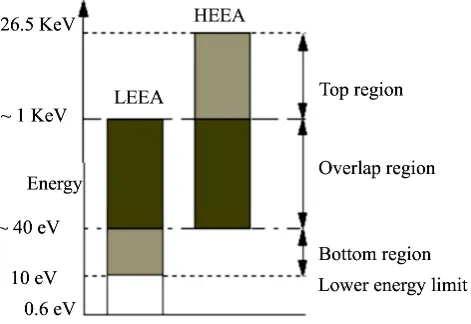
The Plasma Electron and Current Experiment (PEACE) on board the Cluster spacecraft consists of two sensors, HEEA (High Energy Electron Analyser) and LEEA (Low Energy Electron Analyser), mounted on diametrically opposite sides of the spacecraft. They are designed to measure the three dimensional velocity distributions of electrons in the range of 0.6 eV to∼ 26 keV. In standard mode, HEEA measures the range of 35 eV to 26 keV and LEEA measures the range of 0.6 eV to 1 keV, although either can be set to cover any

Fig. 2. An example of the energy range coverage for the

combina-tion of the two analysers. The moment calculacombina-tions are calculated from electrons observed with energies of>10 eV, with the bottom region at 10 eV–40 eV, overlap at 40 eV–1 keV and the top region at

>1 keV.

subset of the energy range. Onboard moment calculations are made for energies> 10 eV, with the subsequent energy range divided into 3 regions depending on energy, as shown in Fig. 2. Due to the sensor mounting geometry, the Top and Bottom energy ranges have a 4 s resolution (measured only by HEEA and LEEA, respectively) while the Overlap energy range (measured by both sensors) has a 2 s resolution. We note that data presented in this paper are derived using pre-liminary calibrations. (For further instrument information, the reader is referred to Johnston et al., 1997; Owen et al., 2001, this issue).

3 Observations

3.1 CASE 1: 26 January 2001

In this case, we examine Cluster data for the period 08:00 to 11:00 UT. In Fig. 3, we show the IMF conditions (magnetic field magnitude and 3 GSE coordinates) detected at ACE corresponding to this time period. ACE was∼ 243RE

up-stream of the Earth where the solar wind speed was observed to be∼ 350 km/s. A lag time to Cluster can be calculated using the solar wind speed and distance from ACE to Clus-ter (243RE/350 km/s=74 min). With the 74 min lag time,

we have indicated in Fig. 3 the corresponding positions of events A and F in the Cluster data as shown in Fig. 4. The IMF remains weakly eastward (positive BY), along with a

transition from weakly positive to weakly negativeBZ

6 7 8

B

X GSE

(nT)

ACE MAG DATA, 26 January 2001

0 2 4

B

Y GSE

(nT)

−5 0 5

B

Z GSE

(nT)

06:006 06:30 07:00 07:30 08:00 08:30 09:00 09:30 8

10 <|B|>

(nT)

A F

Time (hr:min) UT

Fig. 3. The IMF conditions detected

by the ACE spacecraft for 26 January 2001. Using a∼74 min lag time calcu-lated from solar wind speed and ACE position, we have marked the region corresponding to the Cluster observa-tions shown in Fig. 4 with red vertical lines.

1 keV). These two ranges give a good indication of the differ-ent ambidiffer-ent plasma populations, with typical magnetospheric electron energies (∼keV) covered by the Top region and the lower energy, magnetosheath electrons (∼ 10’s–100’s eV) covered by the Overlap region. The lower panel shows an energy spectra generated from a combination of both HEEA and LEEA sensors from the zone 11 anode, which records electrons travelling in the +Z GSE direction. These en-ergy vs time spectra are presented in a differential number flux (#/cm2s str eV) as indicated by the colour bar on the right, with energy given in electron volts. We note the very high fluxes below 10 eV are due to spacecraft secondary- and photo-electrons. The position of the spacecraft at the bottom of the figure is shown in GSE coordinates.

At the start of the interval shown in Fig. 4, the spacecraft are located in the plasma mantle, and observe characteristi-cally low plasma densities with energies up to about 100 eV. At 08:20 UT, marked A in the figure, the spacecraft observes an increase in electron density along with spectral properties showing an injection of magnetosheath-like plasma, with en-ergies up to 200 eV. The spacecraft position at this time was 77.3◦invariant latitude and 14.6 MLT. For the upstream IMF conditions described in Fig. 3 (positiveBY andBZ), these

positions place Cluster within the exterior cusp region de-scribed by Fung et al. (1997), (12.8 MLT±2.1 hours, 81◦_).

The plasma characteristics described above are also consis-tent with observations of the cusp region (Newell and Meng, 1992). In Fig. 4 at 08:26 UT, Cluster observes a reduction in density from “cusp” values (but greater than lobe values) and also a reduction in peak spectral flux by a factor O(100). For this preliminary study, we interpret this behaviour as a result of Cluster briefly skimming the duskside flank of the exterior cusp (Fung et al., 1997) and entering the low latitude boundary layer (LLBL) (Newell and Meng, 1992). Between 08:40 UT (marked B) and 09:12 UT (marked C), Cluster ob-serves of a series of brief transitions lasting∼min into a

re-gion with much higher energy electrons (up to 10 keV), as-sociated with a drop-out in the lower energy, magnetosheath-like electrons (< 200 eV). These observations are consis-tent with the boundary plasma sheet (BPS, e.g. Newell and Meng, 1992). Therefore, we infer that the spacecraft make multiple transient encounters with the boundary between the two plasma populations, signified by the bursty nature of the spectra in which the energetic magnetospheric electrons trapped on closed field lines alternate with a less energetic magnetosheath electron population on open field lines. We note that these events are the opposite of the encounters dis-cussed by Lockwood et al. (2001, this issue) where the Clus-ter spacecraft are predominantly in the BPS, making brief excursions into the LLBL. Between 09:12 (marked C) and 09:20 UT (marked D), Cluster observes dense, lower energy electrons, indicated by the increase in the Overlap density, accompanied by a reduction in the photoelectron popula-tion, suggesting an entrance into the magnetosheath (when compared to the population observed in the magnetosheath proper after 10:30 UT). From 09:20 UT (D) until∼09:54 UT (marked E), a further series of transient encounters with BPS-like plasma occurs. Between these encounters, the density is much more magnetosheath-like, when compared to the observations between B and C. This suggests transient en-counters between the BPS and the magnetosheath. From 09:54 UT (E) until about 10:30 UT (marked F), Cluster ob-serves variations similar to those observed between B and C. Just before 10:30 UT (marked F), observations of a strong density enhancement of lower energy electrons signifies the entrance into the magnetosheath proper.

103 104 105 106 107

#/cm

2

s str eV

0.01 0.1

1

#/cm

3

TOP Density 1

10 _#/cm

3

Overlap Density

2001/02610

0

101 102 103

Energy [eV]

08:00 08:30 09:00 09:30 10:00 10:30

A B C D E F

2.2 5.7 8.7

UT

X GSE (RE) Y GSE (RE) Z GSE (RE) 2.7

6.1 8.9

3.3 6.5 9.0

3.7 6.9 9.1

4.3 7.3 9.1

4.8 7.6 9.1

Fig. 4. The density moments and energy spectra from 26 January 2001, 08:01–11:50 UT. The upper panel shows density from the Top

energy region in black and the Overlap energy range in red. The spectrogram is a combination of the HEEA and LEEA sensor, measured in a differential number flux (#/cm2s str eV). We note the large band of photoelectrons below∼10 eV.

the large deviations in BXand BZjust after 09:10 UT

corre-spond to the magnetosheath entry between C and D in Fig. 4. This is followed by a region of rapid magnetic fluctuations that end around 10:00 UT, coinciding with the appearance of the lower energy population recorded by PEACE, marked E in Fig. 4. The region of less rapid magnetic fluctuations between 10:00 UT and 10:30 UT corresponds to the inter-val E to F in Fig. 4. The rotation in BX andBZ just

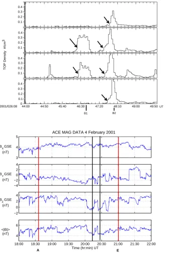
af-ter 10:30 UT corresponds to the entry of the magnetosheath proper observed in the electron data. We note the signifi-cant magnetic field structure after 10:30 UT and the lack of features in the corresponding electron data. An analysis of these features along with the overall crossing will be pre-sented elsewhere. We now focus on the period just after the entry into the boundary layer at the time marked B in Fig. 4. In Fig. 6, we again show combined HEEA and LEEA spec-tra in a differential number flux (#/cm2 s str eV) this time from all 4 spacecraft (Cluster 1 (Rumba) at the top, through to Cluster 4 (Tango) at the bottom) for the 5 min period, 08:44–08:49 UT. Differences in measurements from each of the 4 spacecraft are immediately apparent. A flux enhance-ment centred∼08:46:45 UT (labelled B1) is detected only at Cluster 2 and 3, while the feature centred∼08:48:00 UT (labelled B2) is detected at all four spacecraft. Figure 7 cov-ers the same period but in this case, we display only the Top density moments from each spacecraft (Cluster 1 in the top panel through to Cluster 4 in the bottom panel), which give a

good indication of the trapped magnetospheric electron pop-ulation (energy> 1 keV), as discussed above. We note the additional features at 08:45:00 and 08:48:30 UT seen only at Cluster 3 (with possible correlated features in Cluster 2). 3.2 CASE 2: 4 February 2001

In this case, we examine Cluster data for the period of 08:00 to 11:00 UT. The corresponding IMF conditions recorded at ACE are shown in Fig. 8. The solar wind conditions were quiet at this time with a bulk speed of around (320 km/s). Using a similar method to case one, we calculate a lag time to Cluster of∼84 min and have indicated with the vertical red lines the corresponding position of A and E in the Cluster data shown in Fig. 9. From this region we can see that during the Cluster passage, the IMF is persistently northward but sees several changes in the direction ofBZ. We present an

−40 −20 0 20

B_X GSE (nT)

Cluster Magnetic Field 26 January 2001

−40 −20 0 20

B_Y GSE (nT)

−40 −20 0 20

B_Z GSE (nT)

08:000 08:30 09:00 09:30 10:00 10:30

10 20 30 40 <|B|>

(nT)

2.2 5.7 8.7

2.7 6.1 8.9

3.3 6.5 9.0

3.7 6.9 9.1

4.3 7.3 9.1

4.8 7.6 9.1

X GSE (RE) Y GSE (RE) Z GSE (RE)

A B C D E F

UT

Fig. 5. Magnetic field data from the

Flux Gate Magnetometer (FGM). The plot notation is the same for Fig. 3. The

BXandBZcomponents show large de-viations just after 09:10 corresponding to the low energy plasma enhancement at “C” in Fig. 4.

102 103

102 103

102 103

Energy [eV]

2001/02610 1 102

103

08:44 08:45 08:46 08:47 08:48 08:49

103

104

105

106

#/cm

2

s

str

eV

UT

B1 B2

Figure 6

Fig. 6. Spectra from all four space-craft from 26 January 2001, 08:44– 08:49 UT, focusing on the region B in Fig. 3. Again, the spectra are a combi-nation of the HEEA and LEEA sensors, with Cluster 1 at the top and Cluster 4 at the bottom. The feature at∼08:46:41 (labelled B1) is detected only at Clus-ter 2 and 3, followed by the event at

∼08:48:01 (labelled B2) detected at all

four spacecraft.

we generalise the definition of the cusp given by Fung et al. (1997) and Eastman et al. (2000). We take the cusp to be a region of relatively depressed magnetic field magnitude (Far-rell and Van Allen, 1990), with electron energies approach-ing 1 keV consistent with a mixture of magnetosheath and magnetospheric electrons (Eastman et al., 2000). Around 21:41 UT, marked B, Cluster observes an isolated burst of energetic electrons, which registers a significant increase in the Top density and a large drop-out in the Overlap density. Just before 22:02 UT, marked C, there is a significant de-crease in the Top density followed by two transient inde-creases (up to 22:15 UT, marked D), suggesting short duration en-tries into the magnetosheath and then a final increase back to the energies comparable to those observed between A and B.

However, we note that the region C–D retains some higher energy electrons, as indicated by the Top density which de-creases, but not to the levels detected in the magnetosheath proper after 22:25 UT (E).

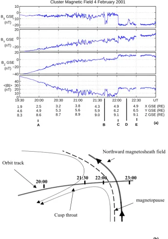
As in Case 1, we gain further insight into the position of the spacecraft at this time by using magnetic field data from the FGM sensor, as shown in Fig. 10a. A smooth reduc-tion in the magnitude of theBZcomponent of the magnetic

field with rather constantBXand a depressed magnetic field

0.1 0.2 0.3 0.4

0.1 0.2 0.3 0.4

0.1 0.2 0.3 0.4

TOP Density #/cm

3

2001/026:08 0 0.1 0.2 0.3 0.4

44:00 44:50 45:40 46:30 47:20 48:10 49:00 49:50

B1 B2

UT

Figure 7

Fig. 7. A plot of the Top density

mo-ments for each spacecraft, with Cluster 1 in the top panel, through to Cluster 4 in the bottom panel. The trace repre-sents the densities calculated from elec-trons detected above 1 keV. Timing is carried out such that entry is indicated by a change in the gradient of the ramp seen before the main structure, as indi-cated by the arrows. A similar method is used for exit. The entry and exit se-quence is shown in Table 1.

3 4 5

B_X GSE (nT)

ACE MAG DATA 4 February 2001

−4 −2 0 2 4

B

Y GSE

(nT)

−2 0 2 4

18:00 18:30 19:00 19:30 20:00 20:30 21:00 21:30 22:00 4

6 <|B|>

(nT)

Time (hr:min) UT

A E

B_Z GSE (nT)

Fig. 8. IMF conditions from the ACE

spacecraft for 4 February 2001, in GSE coordinates. The solar wind speed at this time was∼ 310 km/s, giving a lag time to Cluster of∼ 84 min. Using this time, we have indicated the extent of the Cluster observations in Fig. 9 by the red vertical lines. From this region we can see that during the Cluster pas-sage, the IMF is northward with sev-eral changes in the direction ofBY. The region bounded by the solid black ver-tical lines corresponds to a∼ 15 min period aroundBin Fig. 9, highlighting two∼ 2 min variations in the IMFBX andBY.

throat of the cusp (Fung et al., 1997). We note the rotation of the magnetic field corresponding to the region of high energy electrons between 21:42 and 21:44 UT (marked B). There are changes in all components of the field, most obviously inBX

and a slight increase in the magnitude of the field. Just after 22:00 UT, there is a large rotation in the field corresponding to C in Fig. 9 followed by a lesser rotation at∼22:15 UT (D). We note the data gap beginning at 22:30 UT, which oc-curs during the period covering the magnetosheath entry ob-served in the electrons, and that the values of the magnetic field data before and after this gap are quite similar. In this

103 104 105 106 107

#/cm

2

s str eV

10-3

10-2

10-1

#/cm

3

TOP Density

10

#/cm

3

Overlap Density

2001/035

101

102

103

Energy [eV]

19:30 20:05 20:40 21:15 21:50 22:25

1.9 4.6 8.3

2.6 5.0 8.6

3.4 5.4 8.8

4.0 5.8 8.9

4.7 6.1 9

5.4 6.4 9.1

UT

X GSE (RE) Y GSE (RE) Z GSE (RE)

A B C D E

Figure 9

Fig. 9. Energy spectra and density moments from 4 February 2001, 19:30–23:00 UT in same format as Fig. 3.

4 Discussion

4.1 Boundary analysis

The tetrahedron configuration of the four cluster spacecraft enables the three dimensional study of small scale structures in space plasma for the first time. In this paper we use the method detailed by Harvey (2000), where the spatial gradi-ent of structures encountered by the spacecraft can be deter-mined by the timings and positions of the 4 spacecraft. We assume that the observed boundary is planar such that the boundary normal and velocity are parallel and that they do not change during the passage of the tetrahedron i.e. uni-form motion. Following Harvey (2000), we calculate R, a symmetric tensor describing the geometric properties of the tetrahedron

Rj k=

1 4

4

X

α=l

rαjrαk. (1)

The following equations can then be used to calculate the velocity and direction of the boundary normal.

ml =

1 4

4

X

α=l

tαrαk

!

R−1

kl, (2)

wherej,kandlare matrix indices,αis spacecraft number and

rα =(rα1, rα2, rα3)

Table 1. Entry and exit sequence of spacecraft for features B1 and

B2 in Figs. 6 and 7

entry sequence exit sequence

B1 2 3 – – 2 3 – –

B2 2 3 4 1 2 3 4 1

whererαandt αare the position and time (with respect to the centre of the tetrahedron) that theαt hspacecraft passes the boundary. Velocity is then given by

v= m

|m|2. (3)

In this preliminary analysis, we have neglected detailed con-sideration of timing and position errors and present the nor-mal direction as a first order approximation of the boundary orientation. This will be improved on in future work. 4.2 CASE 1: 26 January 2001

−20 −10 0 10

B

X GSE

(nT)

Cluster Magnetic Field 4 February 2001

−20 0 20

B

Y GSE

(nT)

−40 −20 0 20

B

Z GSE

(nT)

19:300 20:00 20:30 21:00 21:30 22:00 22:30

10 20 30 40 <|B|>

(nT)

1.9 4.6 8.3

2.5 4.9 8.6

3.2 5.3 8.7

3.8 5.6 8.9

4.3 5.9 9.0

4.9 6.5 9.1

X GSE (RE) Y GSE (RE) Z GSE (RE)

A B C D E

UT

4.9 6.2 9.1

(a)

Orbit track

Cusp throat

Northward magnetosheath field

magnetopause

23:00

21:30 22:00

20:00

(b)

Fig. 10. (a) Magnetic field data from the FGM sensor on Cluster 3 (Samba). Notation is the same for Fig. 9. We note the change after 21:40,

marked B, corresponding to an energetic electron event and the initial entry into the magnetosheath just after 22:00, as inferred from the electron data in Fig. 9. Using this magnetic field data along with the orbit position and MLT data, we propose the orbit path sketched in (b), with the orbit passing directly through the throat of the cusp, with the energetic electron event occurring within this region.

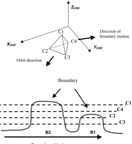
sequence for each spacecraft is identical, i.e. all spacecraft are in the structure for the same length of time (within tim-ings errors, which in this case is 1 satellite spin,∼4 s). The direction of motion is calculated to be in the dusk-tailward direction, as indicated in the upper part of Fig. 13. The entry and exit sequence suggests that the boundary is not moving over the configuration in a breathing or back and forth mo-tion. Instead, the differences between B1 and B2 suggest

102

103

102

103

102

103

Energy [eV]

2001/035

101

102

103

21:40 21:41 21:42 21:43 21:44 21:45 21:46 21:47

103 104 105 106

#/cm

2

s str eV

A B

UT

Fig. 11. This figure shows a

combi-nation of the HEEA and LEEA sen-sors for each spacecraft, Cluster 1 at the top through to Cluster 4 on the bot-tom over time from 21:39 to 21:49 UT. We can see the clear differences in both timing and overall structure of the fea-ture in each spacecraft, with the ex-cited electron region between 21:42 and 21:44 UT, marked A. We note the sec-ondary feature between∼21:44:15 and 21:45 (marked B) observable only in spacecraft 2–4.

0.08 0.16 0.24 0.32

0.08 0.16 0.24 0.32

TOP Density #/cm

3

0.08 0.16 0.24 0.32

2001/035 0 0.08 0.16 0.24 0.32

21:40 21:41 21:42 21:43 21:44 21:45 21:46 21:47

A B

UT

Figure 12

Fig. 12. The Top region of density

(cal-culated from energies electrons with en-ergies of> 1 keV), for time between 21:39–21:48 UT, gives a good indica-tion of the extent of the high energy electron population. We use a similar method as was employed for Case 1 to achieve the entry/exit times indicated in Table 2.

We end the discussion of this case by briefly examining the region observed after B in Fig. 4, where we observe the ap-pearance of magnetosheath plasma at C–D followed by vari-ous transitions between BPS and magnetosheath-like plasma (D–E). Similar transients to those observed between B and C are observed between E and F leading up to the magne-topause crossing at F. TheBZcomponent (GSE) of the IMF

measured at ACE (Fig. 3) began a large negative turn just before 07:48 UT, withBY ∼ 0. Using the lag time

calcu-lated above (74 min), thisBZshift corresponds to 08:52 UT

at Cluster, right in the middle of region B–C in Fig. 4. Due to the basic method of calculating the timing, we cannot in-fer any direct influence of the IMF conditions on the regions

fol-Orbit direction

XGSE

YGSE ZGSE

C1

C4

C3 C2

Direction of boundary motion

Boundary

C4 C1

C2 C3

B2 B1

Boundary Motion

Figure 13

Fig. 13. Diagram in upper panel shows Cluster configuration with

the orbit direction, boundary structure, and dusk-tailward motion in-ferred from timing analysis. The lower panel illustrates the inin-ferred structure of the boundary interaction with Cluster. We propose that the bursty signature is due to the Cluster orbit skimming the bound-ary between the LLBL/magnetosheath and the BPS.

Table 2. Entry and exit sequence of spacecraft for features A and B

from Figs. 11 and 12

entry sequence exit sequence

A 2 4 3 1 2 1 3 4

B 2 3 4 – 2 3 4 –

lowed by a return of BPS/LLBL transitions between E and F, which are again accompanied by a gradual increase in the Overlap density corresponding with the appearance of more magnetosheath-like plasma.

Overall, the electron data describes a noisy and turbulent transit through the dusk side boundary of the cusp. The data from PEACE suggest that Cluster is moving out of the mag-netosphere, duskward of the cusp through a complicated suc-cession of boundary encounters. During this period, ACE ob-served a rotation of the IMF into the negativeBZdirection.

We suggest that this possibly modified the magnetopause in the vicinity of the Cluster spacecraft, further complicating the nature of the magnetopause crossing, inducing a succes-sion of entry/exits from the BPS and LLBL/magnetosheath. 4.3 CASE 2: 4 February 2001

From Figs. 11 and 12, the differences in timing and struc-ture between the four spacecraft measurements are evident.

EXIT NORMAL

ENTRY NORMAL C3

C4 C2

C1 For A-B

Direction of propagation

ZGSE

XGSE YGSE

Entry normal

Exit normal

Direction of Boundary motion

Fig. 14. (a) Illustration of the boundary normal directions for entry

and exit of the structure by Cluster, inferring that a wave-or-bulge like feature is passing over the spacecraft. (b) Projection in the GSE plane (X−Y,Z−Y,Z−X) of the boundary normal directions of the entry (red) and exit (black) of event A. We note that the arrows also indicate the velocity magnitude, such that the entry velocity (red)∼10 km/s, was smaller than exit (black)∼40 km/s. (c) This difference in velocities can be described by the waveform shown here, with a shallow leading edge and steep trailing edge.

For example, the feature marked at B is not present in space-craft 1. We use the above analysis technique to determine the entry and exit sequence using the Top densities shown in Fig. 12. Unlike the previous case, we find that the entry and exit sequences, shown in Table 2, are not the same, indicating that the exit boundary normal of the structure is orientated differently to that of the entry. The rotation of the bound-ary normal from entry to exit can be explained in terms of a wave or quasi-cylindrical structure passing over the space-craft, as shown in Fig. 14a. The motion of this structure is directed duskward towards the tail, as indicated in Fig. 14b, where we show the projection of the entry and exit directions of feature A in each GSE plane (X−Y,Z−Y,Z −X), with entry in red and exit in black. The duskward direction of motion can clearly be seen. The size of the arrows indicate the magnitude of the velocity, where the entry velocity was found to be∼10 km/s and the exit velocity∼40 km/s. This suggests the feature to have a geometry shown in Fig. 14c, with a shallow leading edge and a steeper tail.

in Case 1. Indeed, one may compare the event at 21:45 UT (B) in Fig. 9 to the event just before 09:00 UT in Fig. 4, with an increase in the Top densities and a decrease in the Overlap densities common to both. However, the present case has a well-defined structure, a much longer duration and perhaps most striking, appears to be convecting along the edge of the cusp.

Using the lag time of 84 min calculated above, the appear-ance of the BPS corresponds to∼20:18 UT at ACE, during which time ACE observed a number of changes in IMFBY

and BZas shown in Fig. 8. In particular, we note the

mod-ulations in BY andBZ at∼20:16 and∼20:22 UT with a

duration of∼min, as indicated by the region between the black vertical lines in Fig. 8. Cluster observations imply mo-tion of the cusp throat, most probably due to IMF variamo-tions. The dependence of the cusp location on IMF conditions has been discussed previously by many authors (e.g. Fung et al., 1997; Newell et al., 1989; Zhou et al., 2000). These studies found that for a northward IMFBY <0 (BY >0), the cusp

shifts dawnward (duskward) in addition to a minor deviation equatorward for decreasing positiveBZ. However, from our

approximate lag timings, it is inappropriate to precisely cor-relate motion of the exterior cusp with respect to changes in the IMF on these time scales.

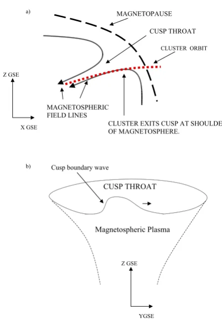
Using a combination of the position of the spacecraft (in the throat of the cusp) and the duskward convection of the BPS/magnetospheric plasma structure calculated above, we suggest that Cluster is in the vicinity of the “shoulder” of the magnetosphere bordering the cusp, as shown in Fig. 15a. The observed transient entry of the BPS/magnetosphere is a result of Cluster observing the small-scale structure of the cusp boundary, as shown in Fig. 15b. An obvious candidate for causing this motion is a change in the IMF. A detailed study with accurate timings is required to validate/refute the correlation of these events, but is beyond the scope of this preliminary case study.

5 Conclusion

This work has highlighted two events from the northern dusk side, high-latitude magnetosphere/magnetosheath boundary. These events rely on preliminary calibrations of electron data from the PEACE instrument on board Cluster.

In the first case from 26 January 2001, we have presented data from a time where Cluster is flying through alternat-ing BPS and LLBL/magnetosheath plasmas. The traversal of these regions is characterised in the electron data by succes-sive observations of magnetospheric plasma, with a higher energy and lower density, followed by LLBL/magnetosheath plasma, with lower energy and higher density. The data from the magnetometer suggest that Cluster is duskward and slightly poleward of the cusp. In this work, we have focused on a region where initially the Cluster spacecraft are strad-dling a boundary between the 2 populations (event B1 in Figs. 6 and 7), such that at one point, only 2 of the spacecraft cross over the boundary. Numerous crossings follow this

a) _MAGNETOPAUSE

MAGNETOSPHERIC FIELD LINES

CLUSTER EXITS CUSP AT SHOULDER OF MAGNETOSPHERE.

CLUSTER ORBIT

CUSP THROAT

Z GSE

X GSE

b) Cusp boundary wave

CUSP THROAT

Magnetospheric Plasma

Z GSE

YGSE

Fig. 15. (a) The diagram shows the cusp viewed from dawn in the X−Zplane, with the solar wind flowing from the right. The ap-pearance of BPS plasma in the cusp suggests an entry into the mag-netosphere, as indicated. However, the different orientation of the entry and exit by Cluster to/from the BPS suggests that the transient entry into the BPS is due to a wave-like structure travelling along the equatorward edge of the cusp as in (b). Here, we suggest that the rotation of the IMF modifies the equatorward cusp boundary layer, such that Cluster observes a magnetospheric population convecting duskward along the equatorward edge of the cusp.

event, with the entire tetrahedron traversing the boundary on several occasions. The nature and rapidity of these crossings suggest that Cluster is skimming very close to the boundary. Assuming the boundary to be planar, we find the ordering of the entry and exit sequence of the magnetospheric popula-tions to be identical, suggesting the same boundary normal and direction of motion. This discounts the possibility of the boundary “breathing” back and forth over the spacecraft, and points more towards a boundary wave with very steep edges (as indicated in Fig. 13). In addition, we have tenta-tively linked a change in the IMF direction to a change in the plasma conditions detected at Cluster, suggesting a change in the position of the magnetopause and a resultant change in plasma characteristics, i.e. appearance of magnetosheath-like plasma.

was on a region of electron data with significantly enhanced energy (similar to the BPS plasma population observed in Case 1), which is unlike any other plasma population de-tected elsewhere throughout the entire pass. Using the pla-nar boundary assumption, we determined the entry and exit sequence. However, in this case, they are not the same. In-stead, the normal direction changes, such that the structure describes a cylindrical or wave-like configuration, travelling duskward and tailward. The IMF orientation is northward in this case, with several changes in the orientation and magni-tude ofBY andBZ(GSE), which we associate with the time

period under scrutiny by taking a 84 min time lag. In partic-ular, we note 2 periods around∼20:18 UT, where the vari-ations inBY andBZ occur over a time scale similar to that

of the transient event at Cluster. We suggest that the posi-tion of Cluster with respect to the equatorward cusp bound-ary permits the fortuitous observation of a magnetospheric population convecting duskward along the equatorward edge of the cusp. Due to our basic calculation of lag time, we do not attempt to directly correlate precise IMF changes with observations at Cluster. However, given the time scale and appearance of these observations we suggest that the IMF changes may have had some effect.

The analysis and explanation of the two cases presented in this work and many similar examples require much more study to validate the suggested explanations as to their ori-gin, in particular the effect of IMF variation, and will be pre-sented elsewhere. However, we conclude that they are excel-lent examples of the potential of the Cluster experiment in unlocking the 3-dimensional picture of the magnetospheric system.

Acknowledgements. The authors would like to thank the two ref-erees for their helpful comments and observations during the sub-mission process of this paper. We gratefully acknowledge the work from the engineering and operations teams at UCL/MSSL in build-ing the PEACE experiment as well as the FGM team. We also ac-knowledge the Bartol Research Institute (BRI) and Norman F. Ness, Los Alamos National Laboratory and D. J. McComas and particu-larly the help from R. Skoug for use of the level 2 ACE MAG and ACE Solar Wind Experiment data respectively. This work has been supported in the UK by the UCL/MSSL PPARC Rolling grant.

Topical Editor G. Chanteur thanks two referees for their help in evaluating this paper.

References

Balogh, A., Dunlop, M., et al.: The Cluster Magnetic field experi-ment, Space Science Reviews 79, 65–91, 1997.

Balogh, A., Carr, C. M., Acu˜na, M. H., et al.: The Cluster magnetic field investigation: overview of in-flight performance and initial results, Ann. Geophysicae, this issue, 2001.

Chen, S.H., Boardsen, S. A., Fung, S. F., Green, R. L., Kessel, R. L., Tan, L. C., Eastman, T. E., and Craven, J. D.: Exterior and interior polar cusps: Obervations From Hawkeye, J. Geophys. Res., 102, No. A6, 11, 335–347, 1997.

Dunlop, M. W., Cargill, P., Stubbs T., and Woolliams, P.: The high altitude Cusps: HEOS-2, J. Geophys. Res., 105, 27, 509–517, 2000.

Eastmann, T. E., Boardsen, S. A., Chen, S.-H., and Fung, S. F.: Configuration of high-latitude and high-altitude boundary layers, J. Geophys. Res., 105, A10, 23 221–23 238, 2000.

Farrell, W. M. and Van Allen, J. A.: Observations of the Earth’s polar cleft at large radial distances with the Hawkeye 1 satellite, J. Geophys. Res., 95, 20 945, 1990.

Fung, S. F., Eastman, T. E., Boardsen, S. A., and Chen, S.-H.: High-altitude Cusp positions sampled by the Hawkeye satellite, Phys. Chem. Earth, 22, 7–8, 1997.

Haerendel, G., Paschmann, G., Sckopke, N., and Rosenbauer, H.: The Frontside Boundary layer of the Magnetopause and the Prob-lem of Reconnection, J. Geophys. Res., 83, 1978.

Harvey, C. H.: Spatial gradients and the Volumetric Tensor, in: Analysis Methods for Multi-Spacecraft Data, (Eds) Paschmann, G. and Daly, P., ISSI, ESA publications division, 1998. Hedgecock, P. C. and Thomas, B. T.: HEOS Observations of the

Configuration of the Magnetosphere, Geophys. J. R. Astr. Soc., Vol. 41, 1975.

Johnston, A. D., Alsop C., et al.: PEACE: a Plasma electron and current experiment, Space Science Reviews, 79, 351–398, 1997. Kessel, R. L., Chen, S.H., Green, J. L., Fung, S. F., Boardsen, S. A., Tan, L. C., Eastman, T. E., Craven, J. D., and Frank, L. A.: Evidence of highaltitude reconnection during northward IMF: Hawkeye observations, 23, 5, 583–586, 1996.

Lockwood, M., Fazakerley, A., Opgenoorth, H., Moen, J., van Eyken, A. P., Bosqued, J.-M., Lu, G., Eglitis, P., McCrea, I. W., Cully, C., Hapgood, M. A., Wild, M. N., Stamper, R., Tay-lor, M., Wild, J., Provan, G., Amm, O., Kauristie, K., Pulkki-nen, T., Strømme, A., Prikryl, P., Pitout, F., Dunlop, M., Balogh, A., R`eme, H., Behlke, R., Denig, W., Hansen, T., Greenwald, R., Morley, S. K., Alcayd´e, D., Blelly, P.-L., Donovan, E., En-gebretson, M., Lester, M., Waterman, J., and Marcucci, M. F.: Coordinated Cluster and ground-based instrument observations of transient changes in the magnetopause boundary layer during northward IMF: relation to reconnection pulses and FTE signa-tures, Ann. Geophysicae, this issue, 2001.

Merka, J., Safrankova, J., Nemecek, Z., et al.: High-altitude cusp: INTERBALL observations, Adv. Space Res., 25, No. 7–8, 1425– 1434, 2000.

Newell, P. T., Meng, C.-I., Sibeck, D. G., et al.: Some low-altitude cusp dependencies on the interplanetary magnetic field, J. Geo-phys. Res., 94, 8921–8927, 1989.

Newell, P. T. and Meng, C.-I.: Mapping the dayside ionosphere to the magnetosphere according to particle precipitation character-istics, Geophys. Res. Lett., 19, 6, 609–612, 1992.

Owen, C. J., Fazakerley, A. N., Carter, P. J., et al.: Cluster PEACE observations of electrons during magnetosphere flux transfer events, Ann. Geophysicae, this issue, 2001.

Russell, C. T.: Polar Eyes the Cusp, Proc. Cluster-II workshop on multiscale / multipoint plasma measurements, London, 22–24 September 1999, ESA SP-449, 47, 2000.

Sandahl, I., Popielawska, B., Budnick, Yu., et al.: The cusp as seen from INTERBALL, Proc. Cluster-II Workshop on Multi-scale/Multipoint Plasma Measurements, London, 22–24 Septem-ber 1999, ESA SP-449, 39–45, 2000.

Zelenyi, L. M., Trska P., and Petrukovich, A. A.: INTERBALL – dual probe and dual mission, Adv. Space Res., 20, 4/5, 549–557, 1997.