Bulletin of Mathematical Analysis and Applications ISSN: 1821-1291, URL: http://www.bmathaa.org Volume 4 Issue 4 (2012), Pages 56-66
INTEGRAL OPERATORS CONTAINING SHEFFER POLYNOMIALS
(COMMUNICATED BY VIJAY GUPTA)
SEZG˙IN SUCU AND ˙IBRAH˙IM B ¨UY ¨UKYAZICI
Abstract. The aim of the present paper is to introduce new type integral operators which involve Sheffer polynomials. We investigate approximation properties of the our operators with the help of the universal Korovkin-type property and also establish the rate of convergence by using modulus of conti-nuity, second order modulus of smoothness and Petree’s K- functional. More-over, some examples which include Sheffer type sequence known as monomial, Bell, Toscano and Laguerre polynomials are given to compute error estimation by modulus of continuity.
1. Introduction
The main aim of an approximation theory is to present nonarithmetic quantities by arithmetic quantities so that the correctness can be determined to a desired degree. In 1953, Korovkin discovered the most powerful and simplest criterion in order to decide approximation process with positive linear operators on continuous functions space. After this year a considerable amount of research has been done by several mathematicians.
Mazhar and Totik [5] modified the Sz´asz operator [6] and defined another class of positive linear operators
Sn∗(f;x) :=ne−nx
∞ X
k=0
(nx)k
k! ∞ Z
0
e−nt(nt) k
k! f(t)dt (1.1)
for functionf which is of exponential type.
Jakimovski and Leviatan [4] introduced a generalization of Sz´asz operators in-cluding Appell polynomials. Let us remind these operators. It is known that the Appell polynomialspk(x) can be defined by
g(u)eux=
∞ X
k=0
pk(x)uk (1.2)
0
2010 Mathematics Subject Classification: 41A25, 41A35.
Keywords and phrases. Sz´asz operators, Modulus of continuity, Korovkin’s theorem, Sheffer polynomials, Toscano polynomials.
c
2012 Universiteti i Prishtin¨es, Prishtin¨e, Kosov¨e. Submitted 23 April, 2012. Accepted 30 October, 2012.
where g(z) = P∞
n=0
anzn is an analytic function in the disk |z| < R (R >1) and g(1)6= 0. From the generating functions (1.2),
Pn(f;x) := e −nx g(1)
∞ X
k=0
pk(nx)f
k
n
is defined by Jakimovski and Leviatan. Ciupa [1] modified the operator Pn as follows
Pn∗(f;x) := e−nx g(1)
∞ X
k=0
pk(nx) n
λ+k+1
Γ (λ+k+ 1) ∞ Z
0
e−nttλ+kf(t)dt (1.3)
where Γ is gamma function and λ≥0. For the special case g(z) = 1 andλ= 0, the operators defined by (1.3) become operatorsS∗
n.
Letpk(x) be Sheffer polynomials defined by
A(u)exH(u)= ∞ X
k=0
pk(x)uk (1.4)
where
A(z) = ∞ X
n=0
anzn , (a 06= 0)
H(z) = ∞ X
n=1
hnzn , (h
16= 0) (1.5)
and suppose that
(i) Forx∈[0,∞) andk∈N∪ {0}, pk(x)≥0,
(ii) A(1)6= 0 andH′(1) = 1, (1.6)
(iii) (1.4) relation is valid for |u|< Rand the power series given by (1.5) converge for |z|< R,(R >1).
Under the assumption (1.6), Ismail [3] introduced and throughly investigated the positive linear operators
Tn(f;x) := e−
nxH(1) A(1)
∞ X
k=0
pk(nx)f
k n
(1.7)
whenever functionf is an exponential type. Now we will revise the operatorTn as follows
Tn∗(f;x) :=e−
nxH(1) A(1)
∞ X
k=0
pk(nx) n
λ+k+1
Γ (λ+k+ 1) ∞ Z
0
e−nttλ+kf(t)dt (1.8)
where the parameterλ≥0.ForH(t) =t, the operatorsT∗
n reduce toPn∗ given by
(1.3).
In the present paper, in order to get more general approximation operators we use Sheffer polynomials and gamma functions.
The structure of this paper as follows. In section 2, we study convergence of the operatorsT∗
n with the help of the universal Korovkin-type property, furthermore
of continuity and Peetre’s K-functional. Finally, in the last section we give some examples of these type operators (1.8) including monomial polynomials, Bell poly-nomials, Toscano polynomials and Laguerre polynomials and also obtain numerical error estimation by using Maple13 for getting new type operators.
2. APPROXIMATION PROPERTIES OF T∗
n OPERATORS
Now we are going to give some auxiliary definitions and lemmas before state our main theorems. Let us define the classE as follows
E:=
f :x∈[0,∞), f(x)
1 +x2 is convergent asx→ ∞
.
Lemma 2.1. T∗
n operators satisfy the following equalities
Tn∗(1;x) = 1 (2.1)
T∗
n(ξ;x) = x+
1
n 1 +λ+ A′(1)
A(1) !
(2.2)
Tn∗ ξ2;x
= x2+x
n 2λ+ 4 + 2 A′(1)
A(1) +H
′′
(1) !
+1
n2 (λ+ 1) (λ+ 2) +
2 (λ+ 2)A′(1) +A′′(1)
A(1)
!
. (2.3)
Proof. Using the generating functions (1.4) and properties of gamma function, we
get above results simply.
Lemma 2.2. For T∗
n operators, the below equality is verified Tn∗
(ξ−x)2;x=xH
′′
(1) + 2
n +
(λ+ 1) (λ+ 2)A(1) + 2 (λ+ 2)A′(1) +A′′(1)
n2A(1) .
(2.4)
Proof. From the linearity of T∗
n operators and applying Lemma 2.1, one can find
(2.4).
Definition 2.1. The modulus of continuity of a functionf ∈C˜[0,∞)is a function
ω(f;δ)defined by the relation
ω(f;δ) := sup |x−y|≤δ
x,y∈[0,∞)
|f(x)−f(y)|
whereC˜[0,∞)is uniformly continuous functions space.
Definition 2.2. The Peetre’s K-functional is defined by
K(f;δ) := inf
g∈W2
∞
n
kf −gkC˜B+δkgkW2
∞
o
whereW2 ∞:=
n
g∈CB˜ [0,∞) :g′, g′′∈CB˜ [0,∞)o,with the norm
kfkW2
∞ :=kfkC˜B+ f
′
˜
CB +
f
′′
˜
CB and the second order modulus of smoothness is defined as
ω2(f;δ) := sup 0≤h≤δ
sup
x∈[0,∞)|
It is known that there is connection between the second order modulus of smoothness and Peetre’s K-functional as follows[1]:
K(f;δ)≤Mnω2
f;√δ+ min (1, δ)kfkC˜B
o
whereM is absolute constant andCB˜ [0,∞)is the class of real valued functions de-fined on[0,∞)which are bounded and uniformly continuous with the normkfkC˜B :=
sup
x∈[0,∞)| f(x)|.
Lemma 2.3. (Gavrea and Rasa [2]) Let g ∈ C2[0, a] and {Ln(g;x)}
n≥1 be a sequence of positive linear operators with the property Ln(1;x) = 1. Then
|Ln(g;x)−g(x)| ≤ g
′
r
Ln(t−x)2;x+1 2 g
′′
Ln
(t−x)2;x .
Letfh be the second order Steklov function attached to the functionf.We will use the following result proved by Zhuk [7]: iff ∈C[a, b] andh∈ 0,b−a
2
,then
kfh−fk ≤ 34ω2(f;h) (2.5)
f
′′
h
≤
3 2
1
h2ω2(f;h) . (2.6)
We now deal with the approximation properties of our operators defined by (1.8).
We begin by stating the following fundamental result.
Theorem 2.1. For given f ∈C[0,∞)∩E,
lim
n→∞T ∗
n(f;x) =f(x)
the convergence being uniform in each compact subset of [0,∞).
Proof. By using (2.1),(2.2) and (2.3), we deduce that
lim
n→∞T ∗
n ξi;x
=xi , i= 0,1,2
uniformly on compact subset of [0,∞). Hence, an application of the universal
Korovkin-type property completes the proof.
Usually, the error estimates in approximation theory are provided in terms of modulus of continuity, second order modulus of smoothness and Peetre’s K-functional. So, let us state the order of approximation to function f byT∗
n with
the help of above tools.
Theorem 2.2. If f ∈C˜[0,∞)∩E, then we have
|Tn∗(f;x)−f(x)| ≤(1 +ϑn(x))ω
f;√1
n
where
ϑn(x) = s
x(H′′
(1) + 2) +1
n
(λ+ 1) (λ+ 2) + 2 (λ+ 2)A
′
(1) +A′′
(1)
A(1)
Proof. By using (2.1), property of the modulus of continuity and after some simple calculations, we can write
|Tn∗(f;x)−f(x)|
≤ e−
nxH(1) A(1)
∞ X
k=0 pk(nx)
1 +1
δ
nλ+k+1
Γ (λ+k+ 1) ∞ Z
0
e−nttλ+k|t−x|dt
ω(f;δ) .
Applying the Cauchy-Schwarz inequality for the integral term on the right hand side of the above inequality, we conclude
|Tn∗(f;x)−f(x)| ≤
e−nxH(1) A(1)
∞ X
k=0 pk(nx)
× 1 + 1
δ
r
x2−2 (λ+k+ 1) n x+
(λ+k+ 1) (λ+k+ 2)
n2
!
ω(f;δ)
= (
1 + 1
δ
e−nxH(1) A(1)
∞ X
k=0 pk(nx)
×
r
x2−2 (λ+k+ 1) n x+
(λ+k+ 1) (λ+k+ 2)
n2
)
ω(f;δ) .
(2.7)
If we use again the Cauchy-Schwarz inequality in the above result (2.7), one can obtain the following
|T∗
n(f;x)−f(x)|
≤
1 + 1
δ v u u tH ′′
(1) + 2
n x+
1
n2
(λ+ 1) (λ+ 2)
+2(λ+2)A
′
(1)+A′′(1) A(1)
!
ω(f;δ)
=
1 + 1
δ 1 √ n v u u t(H
′′
(1) + 2)x+1
n
(λ+ 1) (λ+ 2) +2(λ+2)A
′
(1)+A′′(1) A(1)
!
ω(f;δ) .
In the previous inequality, choosingδ= √1
n one can get desired result.
Now, we compute the rate of convergence of the operatorsT∗
n with the help of
the second order modulus of smoothness.
Theorem 2.3. Let f be defined on [0,∞)and f ∈C[0, a], then the rate of con-vergence the sequence of T∗
n is governed by
|Tn∗(f;x)−f(x)| ≤ 2ah2kfk+3
4 2 +a+h
2
ω2(f;h)
whereh:= 4
r
T∗
n
(ξ−x)2;x.
Proof. Let us denote the second order Steklov function of f as fh. Because of
T∗
n(1;x) = 1,one can write
From the Landau inequality and applying (2.6), we may derive the following f ′ h ≤ 2
akfhk+ a 2 f ′′ h ≤ 2
akfk+
3a
4 1
h2ω2(f;h) . (2.9)
By virtue offh∈C2[0, a],if we use the Lemma 2.3, (2.6) and (2.9) we obtain the
estimate
|Tn∗(fh;x)−fh(x)| ≤
2
akfk+
3a
4 1
h2ω2(f;h)
r
T∗
n
(ξ−x)2;x
+3 4
1
h2Tn∗
(ξ−x)2;xω2(f;h) . (2.10)
Choosingh= 4
r
T∗
n
(ξ−x)2;xin inequality (2.10) and then considering the last
statement in (2.8),so the proof is completed.
Furthermore, in the case f is smooth function the following theorem gives the estimation of approximation to functionf.
Theorem 2.4. For f ∈W2
∞, we have
|Tn∗(f;x)−f(x)| ≤
1
nµ(x)kfkW2
∞ (2.11)
where
µ(x) :=x 1 + H
′′
(1) 2
!
+1
2 (λ+ 1) (λ+ 4) +
2 (λ+ 3)A′(1) +A′′(1)
A(1)
!
.
Proof. From the Taylor formula
f(ξ) =f(x) +f′(x) (ξ−x) +f
′′
(η) 2 (ξ−x)
2
whereη∈(x, ξ).Due to linearity property of operatorsT∗
n,one can write Tn∗(f;x)−f(x) =f
′
(x)Tn∗(ξ−x;x) + f′′(η)
2 T ∗
n
(ξ−x)2;x .
From this fact and using Lemma 2.1, we obtain
|Tn∗(f;x)−f(x)| ≤
1
n 1 +λ+ A′(1)
A(1) ! f ′ CB +1 2 (
H′′(1) + 2
n x
+ 1
n2 (λ+ 1) (λ+ 2) +
2 (λ+ 2)A′(1) +A′′(1)
A(1) !) f ′′ CB .
By a simple calculation in the above inequality, we immediately derive (2.11).
The next theorem contains quantitative estimate by means of Peetre’s K-functional.
Theorem 2.5. For every f ∈CB˜ [0,∞),we have
|Tn∗(f;x)−f(x)| ≤2M ω2(f;h) + min 1, h2
kfkC˜B whereh:=
q
Proof. Let beg∈W2
∞. From the previous theorem, it is clear that
|T∗
n(f;x)−f(x)| ≤ 2
(
kf−gkC˜B+ 1
2n
"
1 +H
′′
(1) 2
!
x
+1
2 (λ+ 1) (λ+ 4) +
2 (λ+ 3)A′(1) +A′′(1)
A(1)
!#
kgkW2
∞
)
(2.12)
Because of the left hand side of inequality (2.12) does not depend on function g, the following result satisfies
|Tn∗(f;x)−f(x)| ≤2K
f;µ(x) 2n
.
If we use connection between Peetre’s K-functional and the second order modulus of smoothness, then by choosingh:=
q
µ(x) 2n we get
|Tn∗(f;x)−f(x)| ≤2M ω2(f;h) + min 1, h2
kfkC˜B .
3. EXAMPLES OF THESE TYPE OPERATORS
Example 3.1. The sequence
xk ∞
k=1 which is the Sheffer sequence for A(t) = 1 andH(t) =t has the generating functions following type
ext=
∞ X
k=0 xk
k!t
k .
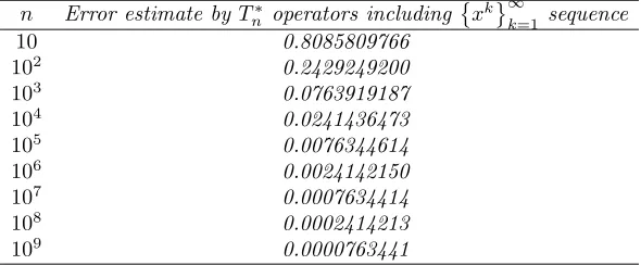
Let us selectpk(x) = xk
k!.Considering these polynomials in(1.8),we find operators as follows
Tn∗(f;x) =e−nx
∞ X
k=0
(nx)k
k!
nλ+k+1
Γ (λ+k+ 1) ∞ Z
0
e−nttλ+kf(t)dt.
If we take λ = 0 in above operators, we get modified Sz´asz operators (1.1) which are defined by Mazhar and Totik[5].
n Error estimate byT∗
n operators including
xk ∞
k=1 sequence
10 0.8085809766
102 0.2429249200
103 0.0763919187
104 0.0241436473
105 0.0076344614
106 0.0024142150
107 0.0007634414
108 0.0002414213
109 0.0000763441
Table 1. The error bound of function f(x) = sin x√1 +x2
Example 3.2. {Bk(x)}which are known as Bell polynomials forms the associated Sheffer sequence forA(t) = 1andH(t) =et−1,so the polynomials have generating
functions
exp x et−1 =
∞ X
k=0 Bk(x)
k! t
k . (3.1)
Furthermore,Bk(x) polynomials are given by
Bk(x) =e−x
∞ X
m=0 mk m!x
m.
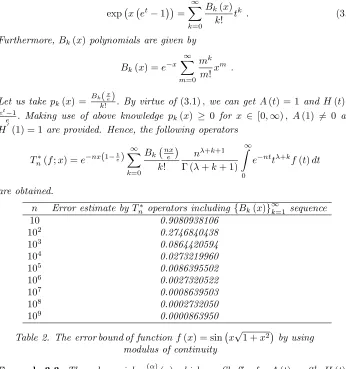
Let us take pk(x) = Bk(xe)
k! . By virtue of (3.1), we can get A(t) = 1 andH(t) = et
−1
e . Making use of above knowledge pk(x) ≥ 0 for x ∈ [0,∞), A(1) 6= 0 and H′(1) = 1are provided. Hence, the following operators
Tn∗(f;x) =e−nx(1−1
e) ∞ X
k=0 Bk nx
e
k!
nλ+k+1
Γ (λ+k+ 1) ∞ Z
0
e−nttλ+kf(t)dt
are obtained.
n Error estimate by T∗
n operators including{Bk(x)}∞k=1 sequence
10 0.9080938106
102 0.2746840438
103 0.0864420594
104 0.0273219960
105 0.0086395502
106 0.0027320522
107 0.0008639503
108 0.0002732050
109 0.0000863950
Table 2. The error bound of function f(x) = sin x√1 +x2
by using modulus of continuity
Example 3.3. The polynomials g(kα)(x)which are Sheffer forA(t) =eαt, H(t) =
1−ethave the generating functions of the form
exp(αt+x(1−et)) = ∞ X
k=0
g(kα)(x)
k! t
k . (3.2)
These polynomials are known as Toscano polynomials or actuarial polynomials, since they were introduced in connection with problems of actuarial mathematics. The relation
gk(α)(−x) =e−x
∞ X
m=0
(α+m)k
m! x
m
stated by Whittaker and Watson. It is clear that for x∈ [0,∞) and α ≥ 0, the
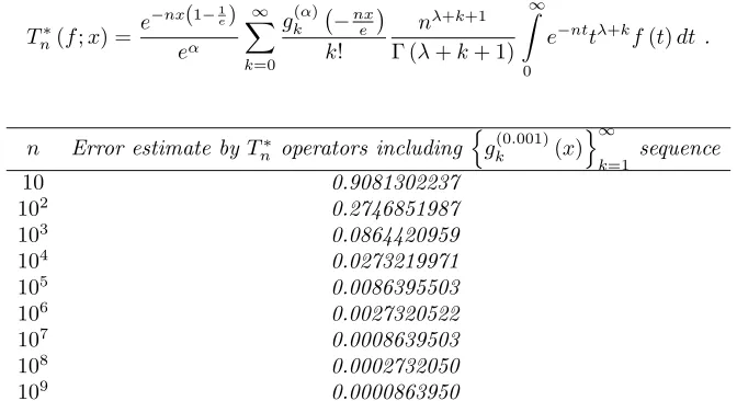
polynomials g(kα)(−x) are positive. Let us choose pk(x) := g
(α)
k (−xe)
By using the above information, pk(x) ≥ 0 (x∈[0,∞), α≥0), A(1) 6= 0 and
H′(1) = 1are satisfied. So, we obtain the following special operators
Tn∗(f;x) = e
−nx(1−1
e)
eα
∞ X
k=0
gk(α) −nx e
k!
nλ+k+1
Γ (λ+k+ 1) ∞ Z
0
e−nttλ+kf(t)dt.
n Error estimate by T∗
n operators including
n
gk(0.001)(x)o∞
k=1 sequence
10 0.9081302237
102 0.2746851987
103 0.0864420959
104 0.0273219971
105 0.0086395503
106 0.0027320522
107 0.0008639503
108 0.0002732050
109 0.0000863950
Table 3. The error bound of function f(x) = sin x√1 +x2
by using modulus of continuity
Example 3.4. Laguerre differential equation is
xy′′+ (1−x)y′+ky= 0
where k is a positive integer. The standard solution of this equation called the Laguerre polynomial of orderk, and is given by
Lk(x) =
k
X
m=0
(−1)mk! (k−m)! (m!)2x
m . (3.3)
Laguerre polynomials satisfy the generating relation
1 1−te
− t
1−tx= ∞ X
k=0
Lk(x)tk . (3.4)
If we consider the above equality, then Laguerre polynomials are Sheffer type poly-nomials. Taking into account of formula (3.3), Laguerre polynomials Lk(−x) are
positive for x ≥ 0. Now, let be pk(x) = Lk(−x2)
2k . Then by virtue of (3.4), one can get A(t) = 2−2t and H(t) = t
2(2−t). From these facts, pk(x) ≥0 for x ≥0, A(1)6= 0 andH′(1) = 1are satisfied. After all, we obtain operators as follows
Tn∗(f;x) =e−
nx
2
∞ X
k=0
Lk −nx 2
2k+1
nλ+k+1
Γ (λ+k+ 1) ∞ Z
0
n Error estimate byT∗
n operators including {Lk(x)}∞k=1 sequence
10 1.0390028560
102 0.3029856656
103 0.0949631527
104 0.0300029998
105 0.0094869278
106 0.0030000029
107 0.0009486833
108 0.0003000000
109 0.0000948683
Table 4. The error bound of function f(x) = sin x√1 +x2
by using modulus of continuity
Algorithm 3.1. The estimates found by following algorithm are given in Table 1. In the Table 1, we establish error estimates for the approximation withT∗
n operators
including
xk ∞
k=1 sequence. restart;
f:=x->sin(x*sqrt(1+xˆ2)); n:=1:
for i from 1 to 9 do n:=10*n;
delta1:=evalf(1/sqrt(n));
omega1(f,delta1):=evalf(maximize(expand(abs(f(x+h)-f(x))),x=0..1-delta1,h=0..delta1)): error1:=evalf((1+sqrt(2+2/n))*omega1(f,delta1));
end do;
Remark 3.1. The algorithms for the numbers obtained in Table 2, Table 3 and Table 4 are pretty similar to the previous one.
Remark 3.2. Because of Bell polynomials, Toscano polynomials and Laguerre poly-nomials are not Appell polypoly-nomials, the operators constructed above aren’t included Ciupa’s article[1].
References
[1] Ciupa, A., A class of integral Favard-Sz´asz type operators, Studia Univ. Babe¸s-Bolyai Math., 40 (1) (1995), 39–47.
[2] Gavrea, I. and Rasa, I., Remarks on some quantitative Korovkin-type results, Rev. Anal. Num´er. Th´eor. Approx., 22 (2) (1993), 173-176.
[3] Ismail, M.E.H., On a generalization of Sz´asz operators, Mathematica (Cluj), 39 (1974), 259– 267.
[4] Jakimovski, A. and Leviatan, D., Generalized Sz´asz operators for the approximation in the infinite interval, Mathematica (Cluj), 11 (1969), 97-103.
[5] Mazhar, S.M. and Totik V., Approximation by modified Sz´asz operators, Acta Sci. Math., 49 (1985), 257-269.
[6] Sz´asz, O., Generalization of S. Bernstein’s polynomials to the infinite interval, J. Research Nat. Bur. Standards, 45 (1950), 239–245.
SEZG˙IN SUCU
Ankara University Faculty of Science, Department of Mathematics, Tando˘gan TR-06100, Ankara, Turkey.
E-mail address: [email protected]
˙IBRAH˙IM B ¨UY ¨UKYAZICI
Ankara University Faculty of Science, Department of Mathematics, Tando˘gan TR-06100, Ankara, Turkey.