Reconfigurable Control of Two-Time Scale Systems in Presence
of Additive Faults
Adel Tellili
1,3,*, Nouceyba Abdelkrim
1,2, Amina Challouf
1,2,
Mohamed Naceur Abdelkrim
1,41 Research Unit MACS, Higher National Engineering School at Gabès, Tunisia; 2 Higher Institute of Industrial Systems at Gabès, University of Gabès, Tunisia;
3 Higher Institute of Technological Studies at Djerba (ISETJB), Tunisia; 4 National Engineering School at Gabès, University of Gabès, Tunisia;
e-mail: [email protected], [email protected], [email protected], [email protected]
http://dx.doi.org/10.5755/j01.itc.44.4.8532
Abstract. This work presents an adaptive approach for fault tolerant control of singularly perturbed systems, where both actuator and sensor faults are examined in presence of external disturbances. For sensor faults, an adaptive controller is designed based on an output-feedback control scheme. The feedback controller gain is determined in order to stabilize the closed-loop system in the fault free case and vanishing disturbance, while the additive gain is updated using an adaptive law to compensate for the sensor faults and the external disturbances. To correct the actuator faults, a state-feedback control method based on adaptive mechanism is considered. The both proposed controllers depend on the singular perturbation parameter ε leading to ill-conditioned problems. A well-posed problem is obtained by simplifying the Lyapunov equations and subsequently the controllers using the singular perturbation method and the reduced subsystems yielding to an ε-independent controller. The control scheme, designed based on the Lyapunov stability theory, guarantees asymptotic stability in presence of additive faults and external disturbances provided the singular perturbation parameter is sufficiently small. Finally, a numerical example is presented to demonstrate the effectiveness of the obtained results.
Keywords: Reconfigurable control; Singularly perturbed systems; Time scale decomposition; Adaptive control; Sensor fault; Actuator fault; Lyapunov equations.
1. Introduction
Systems, where slow and fast dynamic phenomena arise, are called singularly perturbed systems. They model many control systems like robotic systems, mo-tor control systems, chemical processes, convection-diffusion systems and electric circuits. Those systems are distinguished by the existence of a small positive parameter called singular perturbation parameter. It indicates the degree of separation between “slow” and “fast” modes of the system. Such small parameters can be used for modeling machine reactance in power systems, capacitance in electronic and wire inductance control systems. Singular perturbation parameter leads frequently to ill-conditioned results in the system analysis and synthesis methods. In order to handle such problems, a reduction technique, called singular perturbation method, is proposed in the literature. Thus, the full-order system is decoupled into slow and fast subsystems, which makes possible to deal with lower-order systems and consequently to simplify the
malfunctions [8-11]. In contrast, the passive approach, also called reliable control, offers a fixed-parameter controller in order to maintain (at least) stability in occurrence of presumed faults without the need for controller reconfiguration and fault diagnosis scheme [6,9,11,12]. Diverse methods are proposed to design reconfigurable controllers in order to ensure closed-loop stability, even in faulty case. A reliable fault-tolerant control method designed for linear systems using simultaneous stabilization is carried out by Stoustrup and Blondel in [12]. Tellili et al. in [13] developed a reliable H∞ controller for linear time-invariant multi-parameter singularly perturbed system to tolerate sensor faults and to ensure H∞ performance. The full-order system controller is then simplified to three reduced reliable H∞ sub-controllers based on the fast and slow problems through the manipulation of the algebraic Riccati equations. Liu et al. in [14] proposed a H∞ fault tolerant controllers to overcome actuator faults. The authors handle three cases of such faults: normal, loss of efficiency, and outage. The designed H∞ controllers can reduce the degree of conservatism compared with existing methods. Richter and Lunze in [15] developed the fault-hiding approach for linear and Hammerstein systems and used virtual actuators and sensors respectively, for actuator and sensor faults. The results are extended to piecewise affine systems in [8]. Another widely studied method consists in the design of fault tolerant control scheme based on adaptive control principles. Such approaches can be applied without using control restructuring and fault diagnosis procedures [16,17]. Many authors were interested in this subject. In particular, Chen and Saif in [17] designed an adaptive scheme to diagnose and to accommodate actuator faults in linear multi-input single-output (MISO) systems with unknown system parameters. The fault tolerant control problem is resolved using the remaining operative actuators. In [18], a class of adaptive control methods based on output feedback approach in order to stabilize linear systems with complete actuator failures is developed. Jin and Yang in [19] designed a direct adaptive state feedback control approach based on Lyapunov stability theory. The resulting closed-loop system is then asymptoti-cally stable in the presence of actuator faults and external disturbances. The method is extended and improved in [20]. Wang et al. in [21] developed an adaptive output feedback control to accommodate actuator faults including outage, loss of efficiency and stuck. An adaptive fault tolerant controller including a fault estimation error minimization problem is designed by Casavola and Garone in [22]. The consi-dered fault in this case is assumed to be piecewise constant with a slowly varying behavior. For the singularly perturbed systems, their control in presence of actuator failures is investigated by some authors. Liu in [14] developed a controller scheme for singu-larly perturbed systems in presence of actuator satura-tion under the assumpsatura-tion that the fast subsystem is
stable. Xin et al. in [23,24] proposed the reduced-order adjoint systems, by which some methods to estimate the basin of attraction of singularly perturbed systems were developed. In [25], an optimal controller based on state-feedback approach is designed to control non-linear singularly perturbed systems subject to actuator saturation. However, the above-mentioned approaches were limited to actuator saturation and did not consider the loss of efficiency by sensors and actuators.
The main goal of this paper is to design an adaptive fault tolerant control scheme for singularly perturbed systems in presence of external disturbances and additive faults characterized by a loss of effectiveness in sensors and actuators. The remaining part of this work is organized as follows. The system description and preliminaries are presented in Section 2. The fault model and the control problem are formulated in case of sensor faults in Section 3. In Section 4, an adaptive fault tolerant control approach against actuator faults and external disturbances is established. An example of application is developed in Section 5 followed by a conclusion in the last section.
2. System description and preliminaries
Consider the following time-invariant two-time scales singularly perturbed system under external disturbances described by
11 12 1
21 22 1
2 2
1 2
( ) ( )
( )
( ) ( )
( )
( ) ( )
( )
( ) ( )
x
z
x
z
A A B
x t x t
w t
A A B
z t z t
B u t B
x t x t
y t C C C
z t z t
(1)
where
n1x
and
n2z
are state vectors,
mu
is the control vector,
ly
is the output,
qw
models piecewise continuous bounded external disturbances acting on the system and verifying ‖𝑤‖ ≤ 𝑤 with 𝑤 being an unknown positive constant. 1x 111
n n
A , 1x 2
12
n n
A , 212x 1
n n
A ,
2x 2 22
n n
A , 1 1x
n q x
B , 2 1x
n m x
B , 1 2x
n q z
B ,
11 x 1 1
12
l n C
C C
,
21 x 2 2
22
l n C
C C
and
2x 2
n m z
B are constant matrices. The matrix 𝐴22 is
assumed to be nonsingular (standard singularly perturbed systems). The parameter ε, called singular perturbation parameter, is a positive scalar taking values between 0 and 1. Denote throughout the paper:
T TT
i ix iz
B B B for 𝑖 = 1, 2 and ‖(. )‖ the Euclidian
norm of (.).
subsystems of full-order system (1) can be derived by formally setting the singular perturbation parameter ε to zero [2,26]. The slow subsystem is obtained as
1 2
s s s s s s s
s s s s s
x A x B w B u
y C x D u
(2)
where 1
11 12 22 21
s
A A A A A , 1
1 2 22 21
s
C C C A A ,
1 2 22 2
s
D C A B , 1
12 22
is ix iz
B B A A B for 𝑖 = 1, 2; xs, us, and ws are respectively, the slow part of the states,
the control input u, and the disturbance input w. If (𝐴𝑠, 𝐵2𝑠) is stabilizable and (𝐶𝑠, 𝐴𝑠) is detectable,
then there exists a symmetric and positive definite matrix 𝑃𝑠 satisfying the following slow Lyapunov
equation
2
2
( )
( )
T
s s s s s
s s s s s s
A B K C P
P A B K C Q
(3)
where 𝑄𝑠 is any given positive definite symmetric
matrix and 𝐾𝑠 is a static output feedback gain
stabilizing the slow subsystem such that 𝑢𝑠 = 𝐾𝑠 𝑦𝑠.
The closed-loop slow subsystem is then defined by
2 1
( )
s s s s s s s s
x A B K C x B w . (4)
Most often in literature [13,27,28], the following approximation is used: 𝐴𝑠= 𝐴11, 𝐵1𝑠 = 𝐵1𝑥, 𝐵2𝑠 =
𝐵2𝑥 and
C
s
C
1. Consequently, the slow subsystem (2), the slow Lyapunov equation (3) and the closed-loop slow subsystem (4) can be approached respectively, by the equations (5), (6) and (7):11 1 2
s s x s x s
x A x B wB u (5)
11 2 1
11 2 1
( )
( )
T
x s s
s x s s
A B K C P
P A B K C Q
(6)
11 2 1 1
( )
s x s s x s
x A B K C x B w . (7)
Since C is of full rank, it is assumed, without loss of generality, that the output matrix can be transformed to block-diagonal form [29], 𝐶 = [𝐶01 𝐶0
2], where 𝐶1𝑥 and 𝐶2𝑧 describe respectively,
the slow and the fast part of the output. The fast subsystem is given by
22 1 2
2
f f z f z f
f f
z A z B w B u
y C x
(8)
where zf, uf and wf are the fast parts respectively, of the
states, the control input u and the disturbance input w. The fast subsystem can be rewritten in the stretching (fast) time scale 𝑡/𝜀 as follows
22 1 2
2
f f z f z f
f f
z
A z
B w
B u
y
C x
(9)Assuming that (𝐴22, 𝐵2𝑧) is stabilizable and
(𝐶2, 𝐴22) is detectable, there exists a symmetric and
positive definite matrix 𝑃𝑓 satisfying the following fast
Lyapunov equation:
22 2 2
22 2 2
( )
( )
T
z f f
f z f f
A B K C P
P A B K C Q
(10)
where 𝑄𝑓 is any given positive definite symmetric
matrix and 𝐾𝑓 is a static output feedback gain
stabilizing the fast subsystem such that 𝑢𝑓= 𝐾𝑓 𝑦𝑓.
The closed-loop fast subsystem is then defined by:
22 2 2 1
(
)
f z f f z f
z
A
B K C
z
B w
. (11)3. Controller design with respect to sensor
fault
This section will concentrate on the design of an adaptive fault tolerant controller to handle sensor faults in presence of external disturbances.
3.1. Failure model and problem formulation
The sensor faults which have been taken into account in this section involve loss of efficiency. For the output 𝑦𝑖, 𝑖 = 1, . . , 𝑙 , let 𝑦𝑖
𝑓 be the signal issued
from the i-th faulty sensor; accordingly, the sensor-fault model is expressed as follows,
𝑦𝑖𝑓(𝑡) = 𝜌𝑖 𝑦𝑖(𝑡), (12)
where 𝜌𝑖 represents the sensor efficiency factor and
verifies 0 ≤ 𝜌𝑖≤ 𝜌𝑖≤ 𝜌𝑖≤ 1. 𝜌𝑖 and 𝜌𝑖 indicate the
known lower and upper bounds of 𝜌𝑖, respectively.
The case 𝜌𝑖= 𝜌𝑖= 0 describes the completely
interruption of the sensor i. 𝜌𝑖> 0 denotes the case of
partial failure of 𝑦𝑖. If 𝜌𝑖= 𝜌𝑖= 1, then 𝑦𝑖 𝑓
(𝑡) = 𝑦𝑖(𝑡), which depicts the case of no failure. Denoting
𝜌 = 𝑑𝑖𝑎𝑔(𝜌𝑖), 𝑖 = 1, . . , 𝑙, the uniform sensor-fault
model becomes:
𝑦𝑓(𝑡) = 𝜌 𝑦(𝑡). (13)
The assumption that the control signals and disturbances use identical channels is used by many authors [19, 21] to solve robust control problems. Consequently, the following supposition will be held:
𝐵1𝑥 = 𝐵2𝑥 𝐹 and 𝐵1𝑧= 𝐵2𝑧 𝐹, where F is a matrix
with appropriate dimension.
The problem under consideration is to design a control law such that the closed-loop singularly perturbed system is asymptotically stable for any 𝜀 ∈ ]0, 𝜀∗] despite the sensor fault occurrence and
disturbance.
3.2. Controller proposal for the full-order singularly perturbed system
( ) ( ) x t X z t , 11 12 21 22
( )
A
A
A
A
A
,( )
ix i izB
B
B
for 𝑖 = 1, 2.
System (1) can be expressed as
1 2
( )
( )
( )
( ) ( )
( ) ( )
( )
( )
X t
A
X t
B
w t
B
u t
y t
C X t
(14)By using the sensor-fault model (13) and the hypothesis assumed for the disturbances, system (14) is transformed to
2 2
( )
( )
( )
( )
( )
( ) ( )
( )
( )
X t
A
X t
B
F w t
B
u t
y t
C X t
(15)The proposed fault tolerant controller to stabilize the system (14) is described by:
𝑢(𝑡) = 𝐾1 𝑦(𝑡) + 𝐾2(𝑡) (16)
where K1 is chosen such that ( ( )A
B2( )
K C1 ) isHurwitz and K2(t) is governed by the following update law 2 2 3 2 1
( ) ( )
ˆ
( )
( ( )
( ) ( )
)
T TB
P
X
K t
k t
B
P
X
K CX
(17)
where𝑘̂3 is adjusted using the following adaptive law
3 2 ˆ ( ) ( ) ( ) T dk t
X P B
dt
(18)where γ is a suitable positive constant and ε is the singular perturbation parameter. Let 𝑘̃3(𝑡) = 𝑘̂3(𝑡) −
𝑘3. Then the expression (18) can be transformed to
3( ) ( ) 2( )
T
k t X P B .
As mentioned in [20], to avoid discontinuity which can be caused by the term T ( ) 2( )
X P B in the case where 𝑋 = 0, it is sufficient to add a small constant in the denominator of the control law (17).
The following theorem is proposed to solve the fault tolerant control problem (15):
Theorem 1: Consider the singularly perturbed system described by equation (14). Suppose the following assumptions are satisfied, 1. There exists a singular perturbation
parameter 𝜀∗> 0 such that (𝐴(𝜀), 𝐵
2(𝜀)) is
stabilizable and (𝐶, 𝐴(𝜀)) is detectable for all
𝜀 ∈ ]0, 𝜀∗];
2. There exists a symmetric and positive definite matrix 𝑃(𝜀) satisfying the following Lyapunov equation :
2 1
2 1
( ( )
( )
)
( )
( ) ( ( )
( )
)
TA
B
K C
P
P
A
B
K C
Q
(19)where Q is any given positive definite symmetric matrix;
3. K1 is designed such that ( ( )A
B2( )
K C1 ) is Hurwitz.Then the fault tolerant controller (16) verifying the adaptive laws (17) and (18), stabilizes asymptotically the system (14) subject to sensor fault (13) and external disturbances for any 𝜀 ∈ ]0, 𝜀∗].
Proof. From equations (15) and (16), it follows for the closed-loop fault tolerant control system:
2
2 1 2 2
( )
( )
( )
( )
( )
( )
( )
( )
( )
( )
( )
X t
A
X t
B
F w t
B
K
C X t
B
K t
y t
C X t
(20)which can be rewritten as:
2 1
2 1 2 2
2
( )
( ( )
( )
)
( )
( )
(
)
( )
( )
( )
( )
( )
X t
A
B
K C X t
B
K
I CX t
B
K t
B
F w t
(21)Define an ε-dependent Lyapunov function candidate,
𝑉(𝜀) = 𝑋𝑇 𝑃(𝜀) 𝑋 + 𝜀−1 𝛾−1 𝑘̃
32 > 0. (22)
Computing the derivative of 𝑉(𝜀) along the trajectories of system (21) and taking into account the assumptions about the disturbances leads to
2 1
2 1
1 1
3 3 2 2
2 2 1
( )
[( ( )
( )
)
( )
( ) ( ( )
( )
)]
2
2
( )
( )
2
( )
( )
2
( )
( )
(
)
T T
T
T
T
V
X
A
B
K C
P
P
A
B
K C X
k k
X P
B
K
X P
B
F w
X P
B
K
I CX
(23)Let 𝑘3be a constant used to limit the unknown
bounded constant 𝑤 such that [21]
2 2 3
( )
( )
( )
( )
T TX P
B
F w
X P
B
k
. (24)
Since 𝜌𝑖≤ 1, it can be shown that
2 1 1 2
( )
( )
(
)
( )
( )
T TX P
B
K
I CX
K CX
X P
B
. (25)
2 3
1 2
2 2
3 2
1 1
1 3 3
( )
2
2
( )
( )
2
( )
( )
( )
( )
( ) ( )
ˆ
2
( ( )
( ) ( )
)
2
T T
T
T T
T
V
X Q X
X P
B
k
K CX
X P
B
X P
B
B
P
X
k t
B
P
X
K CX
k k
(26)
This can be transformed into the following form,
2
3 3 1 1
1 1 3 3
( )
2
2
( )
( )
ˆ
(
( )
)
2
T T
V
X QX
X P
B
k
k t
K CX
K CX
k k
(27)In the light of the adaptation law (18), it is easy to see that 𝑉̇(𝜀) ≤ 0. Therefore, the faulty closed-loop system is asymptotically stable for any singular perturbation parameter ε ∈ ]0, ε∗].
3.3. Controller simplification
The fault tolerant controller (16) involves an output feedback gain 𝐾1 designed such that
2 1
( ( )
A
B
( )
K C
)
is Hurwitz. Under mildtechnical conditions, asymptotic stability of the full-order singularly perturbed system is guaranteed through the asymptotic stability of both the slow subsystem and fast subsystem for sufficiently small values of the singular perturbation parameter ε [2,30]. The conception of the static output feedback gain
𝐾1 can be achieved through the simultaneous design
of static output feedback controllers for the reduced slow and fast subsystems for small ε and some constraints on the system [3,30,31]. Thus, a simplified ε-independent feedback controller is designed to stabilize the full-order system.
The approximations taken in Section 2 (see equations (5) and (9)) permit to simplify 𝐵2(𝜀) in the
control law (17) through 𝐵2= [
𝐵2𝑥
𝐵2𝑧]. The ε-dependent
𝑃(𝜀) will be simplified in the following section.
3.4. Solving Lyapunov equation using reduced order models
In order to alleviate the numerical stiffness caused by the simultaneous occurrence of slow and fast phenomena and characterized by the presence of the small singular perturbation parameter ε, the full-order Lyapunov equation (19) will be formulated using slow and fast subsystem components.
The structure of 𝑃(𝜀) is assumed to be of the form
1 2
2 3
( ) PT P
P
P P
. (28)
The solution 𝑃(𝜀) is ɛ-dependent, because equation (19) contains 𝜀−1-order matrices. Let 𝑄 be of
the form 1 1
2
0 0
n n I
Q
I
where 𝐼 is identity matrix and 𝐾1= [𝐾11 𝐾12] . Expanding the Lyapunov
equation (19) after the substitution of 𝑃(𝜀) leads to the following partitioned three equations
1 1
11 1 21 2 1 11 2 21 1
T T T
n
a Pa P P a P a I (29)
1 1
21 3 11 2 1 12 2 22 0
T T
a P a P P a P a
(30)
1 1 1
12 2 22 3 2 12 3 22 2
T T T
n
a Pa PP a P a I (31) where a11A11B K C2x 11 1 , a12A12B K C2x 12 2 ,
21 21 2z 11 1
a A B K C and a22A22B K C2z 12 2.
Pre- and post-multiplying equations (29) and (31) by the singular perturbation parameter ε and letting
ε → 0 leads to the following zero-order equations 11 1 1 11 1
T
n
a PP a I (32)
22 3 3 22 2
T
n
a PP a I (33)
21 2 2 21 0
T T
a P P a . (34)
Since K11 and K12 can be approximated, respectively, by Ks and Kf [29,31], it is clear that
equations (32) and (33) correspond, respectively, to the Lyapunov equations of the slow subsystem approximation described by equations (5) and the fast subsystem given by equation (9) of the singularly perturbed system (1). Hence, 𝑃1 and 𝑃3 correspond,
respectively, to the solution 𝑃𝑠 of the slow Lyapunov
equation (3) (approximated by equation (6)) and the solution 𝑃𝑓 of the fast Lyapunov equation (10). It
follows that the solution 𝑃(𝜀) of the equation (19) can be approximated by ( ) 0
0 s
f P P
P
. Thus, the
ill-defined controller (16) is simplified and made ε-independent using the corresponding reduced order well defined problem.
4. Controller design with respect to actuator
fault
In this section, a fault tolerant controller will be designed to compensate actuator fault and external disturbances and then the singular perturbation method will be used to simplify the ε-dependent controller to avoid the numerical stiffness caused by the presence of time scales.
4.1. Preliminaries and failure model
Consider the LTI singularly perturbed system (1) with its slow subsystem (2) and fast subsystem (9).
If (𝐴𝑠, 𝐵2𝑠) is stabilizable, then the state feedback
controller 𝑢𝑠 = 𝐺𝑠𝑥𝑠 is considered to stabilize the
slow subsystem (2). 𝐺𝑠 is the slow controller gain
satisfying the following slow Lyapunov equation
2 2
( )T ( )
s s s s s s s s s
with 𝑀𝑠 any given positive definite symmetric matrix.
The closed-loop slow subsystem is then obtained
2 1
( )
s s s s s s s
x A B G x B w . (36)
Employing the same approximation used in Section 2 for the system matrices of the slow subsystem, the slow Lyapunov equation (35) and the closed-loop slow subsystem (36) can be approximated, respectively, by the equations (37) and (38):
11 2 11 2
( )T ( )
x s s s x s s
A B G L L A B G M (37)
11 2 1
( )
s x s s x s
x A B G x B w (38)
Assuming that (𝐴22, 𝐵2𝑧) is stabilizable, there
exists a feedback controller 𝑢𝑓 = 𝐺𝑓𝑧𝑓 stabilizing the
fast subsystem (9). 𝐺𝑓 is the fast controller gain
satisfying the following fast Lyapunov equation,
22 2 22 2
(A B Gz f)TLf Lf (A B Gz f) Mf (39)
with 𝑀𝑓 any given positive definite symmetric matrix.
The closed-loop fast subsystem is then described by
22 2 1
(
)
f z f f z f
z
A
B G
z
B w
. (40)The faults dealt with in this section are given by a decrease in effectiveness. For the control input 𝑢𝑖, 𝑖 =
1, . . , 𝑚 , consider 𝑢𝑖𝐹 the signal from the faulty
actuator; consequently, the failure model is adopted as follows
Fi = ai i
u
u
(41)where 𝛼𝑎𝑖 represents the actuator efficiency factor and
verifies 0 ≤ 𝛼𝑎𝑖 ≤ 𝛼𝑎𝑖≤ 𝛼𝑎𝑖≤ 1 . 𝛼𝑎𝑖 and 𝛼𝑎𝑖
indicate the known lower and upper bounds on 𝛼𝑎𝑖,
respectively. Thus, if 𝛼𝑎𝑖 = 𝛼𝑎𝑖= 1, the ith actuator
is working perfectly, whereas if 𝛼𝑎𝑖> 0, partial loss
of effectiveness is present. The case 𝛼𝑎𝑖= 𝛼𝑎𝑖= 0
describes the completely failing of the actuator i. Denoting 𝛼𝑎= 𝑑𝑖𝑎𝑔(𝛼𝑎𝑖), 𝑖 = 1, . . , 𝑚, the uniform
actuator-fault model becomes,
𝑢𝐹(𝑡) = 𝛼
𝑎 𝑢(𝑡) (42)
The problem under consideration is to develop a fault tolerant controller making the closed-loop singularly perturbed system asymptotically stable in presence of actuator faults and external disturbances.
4.2. Controller synthesis for the global singularly perturbed system
Considering the system (14), the actuator fault (42) and the assumption held for the disturbances, system (14) can be rewritten as
2 2
( ) ( ) ( ) ( ) ( ) ( ) a ( ) X t A X t B F w t B u t (43) The proposed controller model to stabilize the system (14) under actuator faults and external disturbances is given by:
𝑢(𝑡) = 𝐺1(𝑡) 𝑋(𝑡) + 𝐺2(𝑡) (44)
where G1 is chosen such that
( ( )
A
B
2( )
G
1)
is Hurwitz and G2(t) is designed using the following update law:2
2 1
2
( ) ( ) ˆ
( ) ( ( ) )
( ) ( ) T
T
B L X
G t k t G X
B L X
(45)
where α and β are appropriate positive constants satisfying [19-21]
2 2
2( ) ( ) 2( ) ( )
T T
a
B L X B L X
(46)
and 𝑘̂ obeys the following adaptive law:
2
ˆ( )
( ) ( )
T
dk t
X L B
dt
(47)where γ is an appropriate positive constant and ε is the singular perturbation parameter. Let 𝑘̃(𝑡) = 𝑘̂(𝑡) − 𝑘, where k is a constant verifying
2
2
( ) ( )
( ) ( ) T
T
X L B F w
X L B k
(48)
then the update law (47) can be expressed as
2
( ) T ( ) ( )
k t X L B (49)
As main result, the following theorem will be proposed to solve the fault tolerant control problem (43),
Theorem 2: Consider the system described by equation (14). Suppose that:
1. There exists a singular perturbation parameter 𝜀∗> 0 such that (𝐴(𝜀), 𝐵
2(𝜀)) is
stabilizable for all 𝜀 ∈ ]0, 𝜀∗];
2. For any given positive definite symmetric matrix M, there exists a symmetric and positive definite matrix 𝐿(𝜀) satisfying the following Lyapunov equation :
2 1
2 1
( ( )
( )
)
( )
( ) ( ( )
( )
)
TA
B
G
L
L
A
B
G
M
(50)3. G1 is chosen such that
( ( )
A
B
2( )
G
1)
isHurwitz.
Then there exists 𝜀∗> 0 such that for every
𝜀 ∈ ]0, 𝜀∗], the controller described by equation (44),
with the update laws (45) and (47) and the controller gain G1, stabilize asymptotically the system (43) subject to actuator fault (42) and external disturbances.
Proof. The Lyapunov-based proof of stability can be shown using the following Lyapunov function candidate
𝑉(𝜀) = 𝑋𝑇 𝐿(𝜀) 𝑋 + 𝜀−1 𝛾−1𝑘̃2 > 0. (51)
4.3. Design of the ε-independent controller
𝐺1 represents the state-feedback controller gain
stabilizing the full-order singularly perturbed system (1) in absence of faults and perturbations. It is well known [2,33] that 𝐺1 can be designed using the locale
feedback gains 𝐺𝑠 and 𝐺𝑓 provided that (𝐴𝑠, 𝐵𝑠) and
(𝐴𝑓, 𝐵𝑓) are controllable and A−122 exists. Accordingly,
the composite control is of the form 𝑢(𝑡) = 𝐺1(𝑡) 𝑋(𝑡) = [𝐺11 𝐺12] [
𝑥
𝑧] where 𝐺12= 𝐺𝑓 and
-1 -1
11 ( f f 22 2
)
s f 22 21G
=
I+
G A B G+
G A A . Thus, the simplification of the feedback controller gain 𝐺1conserves the stability of the full-order singularly perturbed system. To simplify the adaptive laws (45) and (47), it is adequate to use the slow parts of the command matrix 𝐵2(𝜀) and the simplified form of the
Lyapunov matrix 𝐿(𝜀) which will be derived in the following.
4.4. Simplifying of the Lyapunov equation
To remove the numerical stiffness in the Lyapunov equation given by expression (50), the latter will be decomposed in slow and fast parts [34]. The structure of L(ε) is assumed to be of the form
1 2
2 3
( ) LT L
L
L L
. The solution 𝐿(𝜀) is dependent on the singular perturbation parameter ɛ because equation (50) contains 𝜀−1-order matrices. A positive definite
symmetric matrix 𝑀 will be chosen of the form 1
1 2
0
0 n
n I
M
I
, where 𝐼 is identity matrix. Substituting 𝐿(𝜀) into Lyapunov equation (50) yields the following partitioned three equations
1 1
11 1 21 2 1 11 2 21 1
T T T
n
a L a L L a L a I (52)
1 1
21 3 11 2 1 12 2 22 0
T T
a L a L L a L a
(53)
1 1 1
12 2 22 3 2 12 3 22 2
T T T
n
a L a L L a L a I (54) where a11A11B G2x 11 , a12A12B G2x 12 ,
21 21 2z 11
a A B G and a22A22B G2z 12.
Using the same method as in Section 2 yields the following equations
11 1 1 11 1
T
n
a L L a I (55)
22 3 3 22 2
T
n
a L L a I (56)
21 2 2 21 0
T T
a L L a (57)
It is well known that the controller gains 𝐺11 and
𝐺12 can be approximated, respectively, by the slow
controller gain 𝐺𝑠 and the fast controller gain 𝐺𝑓 [35].
Hence, expressions (55) and (56) match respectively, the slow and the fast Lyapunov equations until
𝑀𝑠= 𝐼𝑛1 and 𝑀𝑓= 𝐼𝑛2 . Furthermore, considering
equation (57), the approximate solution of the
Lyapunov matrix becomes ( ) 0 0
s f
L L
L
, which
removes the numerical stiffness in the solution of equation (50).
5. Example of application
To illustrate the effectiveness of the proposed method, the following numerical example is given below.
5.1. Fault tolerant control in presence of sensor faults and disturbance
Consider the singularly perturbed system (1) with parameters given by
11
5 0.2 0.5 6 A
, 12
0 0.1
1 1
A
,
21
9 8
0.3 0.1 A
, 22
7 1
0.5 6 A
,
2 1
1 1.55 1 0.5 0.9 0.8 0.2 0.11
B B
, 2 0.5 0 0
1 2 0 0
C =
and 0.01 sin(5 )
0.5 t w =
.
The full-order system is open loop unstable (the system has one positive pole). The considered faulty model is a 50% loss of effectiveness in the first sensor and 70% in the second sensor, that is, 𝛼𝑎=
𝑑𝑖𝑎𝑔(0.5,0.7). The singular perturbation parameter is set to 𝜀 = 0.05. In the fault free case, the output feedback controller is computed using the method described in [30] based on the reduced order models. The states trajectories starting from 𝑋0=
[0.2, 0.03, 0.02, 0.01]𝑇, the output and the simplified
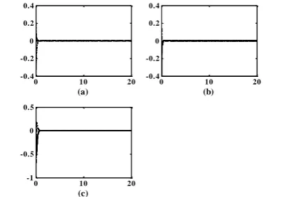
controller gain are shown in Fig. 1. It is clear from the above mentioned figure that the full-order system
Figure 1. (a) States, (b) Output and (c) Controller u(t) in the fault-free case by output feedback control and by ε = 0.05.
0 10 20
-0.4 -0.2 0 0.2 0.4
(a)
0 10 20
-0.4 -0.2 0 0.2 0.4
(b)
0 10 20
-1 -0.5 0 0.5
Figure 2. (a) States, (b) Output and (c) Controller u(t) in the faulty case by output feedback control and by ε = 0.05.
Figure 3. (a) States, (b) Output and (c) Controller u(t) in the faulty case by adaptive fault tolerant control and by ε = 0.05.
is stabilized using the output feedback controller. However, the occurrence of sensor faults at time instance 50 sec causes instability of the full-order system (see Fig. 2). Next, an adaptive fault tolerant controller will be designed in presence of sensor faults and external disturbances. The simulation results are shown in Fig. 3. They indicate that the designed adaptive fault tolerant controller stabilizes asympto-tically the singularly perturbed system subject to sensor faults and external disturbances.
Next, the case of actuator faults will be examined.
5.2. Fault tolerant control in presence of actuator faults and disturbance
The same singularly perturbed system treated below is considered with 10% loss of efficiency in the first actuator and 50% in the second actuator, that is,
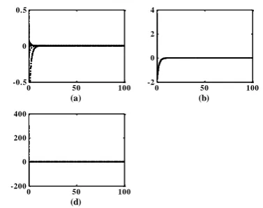
ρ = diag(0.1,0.5). In the fault free case, the full-order system is stabilized through a composite controller based on the slow and fast subsystems (see Fig. 4). The appearance of defects at time 50 sec yields a loss of the actuators performances which is indicated in Fig. 5. To compensate the fault effect, an adaptive fault tolerant controller is designed. Fig. 6 shows the trajectories of the states, the output, the controller 𝑢(𝑡)
and the gain 𝑘3(𝑡) after fault occurrence at time 50 sec
by initial values 𝑋0= [0.2, 0.03, 0.02, 0.01]𝑇 and 𝜀 =
0.05. It can be deduced that the computed adaptive controller compensates the actuator faults in presence of external disturbances.
Figure 4. (a) States, (b) Output and (c) Controller u(t) in the fault-free case by composite control
Figure 5. (a) States, (b) Output and (c) Controller u(t) in the Faulty case by composite control
Figure 6. (a) States, (b) Output, (c) Gain k3(t) and (d)
Controller u(t) in the faulty case by adaptive ftc control
6. Conclusion
In this paper, the stabilization problem of singularly perturbed systems subject to additive faults and external disturbances is investigated. ε-dependent
0 50 100
-1 -0.5 0 0.5 1
(a)
0 50 100
-1 -0.5 0 0.5 1
(b)
0 50 100
-1 -0.5 0 0.5 1
(c)
0 50 100
-0.2 -0.1 0 0.1 0.2
(a)
0 50 100
-0.2 -0.1 0 0.1 0.2
(b)
0 50 100
-10 -5 0 5 10
(c)
0 50 100
-0.5 0 0.5
(a)
0 50 100
-2 0 2 4
(b)
0 50 100
-200 0 200 400
(d)
0 50 100
-2 0 2 4 6
(a)
0 50 100
-5 0 5 10 15
(b)
0 50 100
-20 0 20
(c)
0 50 100
-0.5 0 0.5
(a)
0 50 100
-2 -1 0 1
(b)
0 50 100
0 0.1 0.2 0.3 0.4
(c)
0 50 100
-200 -100 0 100 200
controllers are first proposed to handle sensor and actuator faults covering the normal operation and faulty cases. In both cases, the control scheme includes a feedback controller to handle the fault free case and an adaptive part to compensate additive faults and external disturbances. The resulting Ill-conditioned Lyapunov equation in the two cases is solved using the singular perturbation method and the simultaneous design of Lyapunov equations of the slow and fast subsystems. In the case of sensor faults, the first part of the controller, designed by an output feedback controller, is approximated by gains stabilizing the reduced order systems. While, in occurrence of actuator faults, the state-feedback controller is approximated by a composite controller which depends on the gains stabilizing the slow and fast subsystems. In both cases, the adaptive laws are simplified using ε-independent matrices. The synthesis of the reconfigurable control system guarantees the desired asymptotic stability of the full-order singularly perturbed system not only in the fault-free case, but also in occurrence of additive faults and external disturbances. The determination of the upper bound of singular perturbation parameter ε remains, as perspective, an important thematic.
References
[1] F. El Hachemi, M. Sigalotti, J. Daafouz. Stability analysis of singularly perturbed switched linear systems. IEEE Transactions on Automatic Control, 2012, Vol. 57, No. 8, 2116-2121.
[2] P. Y. Kokotovic, H. K. Khalil, J. O’Reilly. Singular perturbation methods in control- Analysis and design, United States of America, Academic press, Harcourt Brace Jovanovich publishers, 1999.
[3] H. K. Khalil. Output feedback control of linear two-time-scale systems. IEEE Transactions on Automatic Control,1987, Vol. 32, No. 9, 784-792.
[4] D. Bustan, S. K. H. Sani, N. Pariz. Adaptive fault-tolerant spacecraft attitude control design with transient response control. IEEE/ASME Transactions on Mechatronics, 2014, Vol. 19, No. 4, 1404-1411. [5] Y. Wang, P. Zhou, Q. Wang, D. Duan. Reliable
Robust Sampled-Data H-infinity output Tracking Control with Application to Flight Control. Information Technology and Control, 2014, Vol. 43, No. 2, 175-182.
[6] H. Noura, D. Sauter, F. Hamelin, D. Theilliol. Fault tolerant control in dynamic systems: Application to a winding machine. IEEE Control Systems, 2000, Vol. 20, No. 1, 33–49.
[7] R. J. Patton. Fault-tolerant control systems: The 1997 situation. In: Proceedings of theSafe’Process, United Kingdom, 1997, pp. 1033–1055.
[8] J. H. Richter, W.P.M.H. Heemels, N. van de Wouw, J. Lunze. Reconfigurable control of piecewise affine systems with actuator and sensor faults: Stability and tracking. Automatica, 2011, Vol. 47, Nr.4, 678–691. [9] M. L. Corradini, G. Orlando. Actuator failure
identi-fication and compensation through sliding modes. IEEE Transactions on Control Systems Technology, 2007, Vol.15, No. 1, 184−190.
[10] D. Ye, G. H. Yang. Adaptive fault-tolerant tracking control against actuator faults with application to flight control. IEEE Transactions on Control Systems Technology, 2006, Vol. 14, No. 6, 1088−1096. [11] R. Wang, G. Jin, J. Zhao. Robust fault-tolerant
control for a class of switched nonlinear systems in lower triangular form. Asian Journal of Control, 2007, Vol. 9, No. 1, 68−72.
[12] J. Stoustrup, V. D. Blondel. Fault tolerant control: A simultaneous stabilization result. IEEE Transactions on Automatic Control, 2004, Vol. 49, No. 2, 305–310. [13] A. Tellili, M. N. Abdelkrim, M. Benrejeb. Reliable
H∞ control of multiple time scales singularly perturbed systems with sensor failure. International Journal of Control, 2007, Vol. 80, No. 5, 659–665.
[14] L. Liu, Y. Shen, E. H. Dowell, C. Zhu. A general H∞
fault tolerant control and management for a linear system with actuator faults. Automatica, 2012, Vol. 48, 1676-1682.
[15] J. H. Richter, J. Lunze. Reconfigurable control of Hammerstein systems after actuator failures: stability, tracking, and performance. International Journal of Control, 2010, Vol. 83, No. 8, 1612–1630.
[16] W. Wang, C. Wen. Adaptive compensation for infini-te number of actuator failures or faults. Automatica, 2011, Vol. 47, No. 10, 2197-2210.
[17] W. Chen, M. Saif. Adaptive actuator fault detection, isolation and accommodation in uncertain systems. International Journal of Control, 2007, Vol. 80, No. 1, 45–63.
[18] G. Tao, S. H. Chen, S. M. Joshi. An adaptive actuator failure compensation controller using output feedback. IEEE Transactions on Automatic Control, 2002, Vol. 47, No. 3, 506–511.
[19] X-Z. Jin, G-H. Yang. Robust adaptive fault-tolerant compensation control with actuator failures and bounded disturbances. Acta Automatica Sinica, Vol. 35, No. 3, pp. 305-309, 2009.
[20] L-L. Fan, Y-D. Song. On fault-tolerant control of dynamic systems with actuator failures and external disturbances. Acta Automatica Sinica, 2010, Vol. 36, No. 11, 1620-1625.
[21] J. Wang, H.-L. Pei, N.-Z. Wang. Adaptive output feedback control using fault compensation and fault estimation for linear system with actuator failure. International Journal of Automation and Computing, 2013, Vol. 10, No. 5, 463-471.
[22] A. Casavola, E. Garone. Fault-tolerant adaptive con-trol allocation schemes for overactuated systems. International Journal of Robust and Nonlinear Control, 2010, Vol. 20, 1958–1980.
[23] H. Xin, D. Wu, D. Q. Gan, J. J. Qin. A method for estimating the stability region of singular perturbation systems with saturation nonlinearities. Acta Automatica Sinica, 2008, Vol. 34, No. 12, 1549–1555. [24] H. Xin, D. Gan, M. Huang, K. Wang. Estimating the
stability region of singular perturbation power systems with saturation nonlinearities: an linear matrix inequality based method. IET Control Theory and Applications, 2010, Vol. 4, No. 3, 351–361.
[26] K. Datta, A. RaiChaudhuri.H2/H∞ control of singu-larly perturbed systems: The state feedback case. European Journal of Control, 2010, Vol. 16, No. 1, 54-69.
[27] H. K. Khalil, F. C. Chen. H∞ control of two-time-scale systems. Systems and Control Letters, 1992, Vol. 19, No. 1, 35-42.
[28] W. Tan, T. Leung, Q. Tu. H∞ control for singularly perturbed systems. Automatica, 1998, Vol. 34, No. 2, 255-260.
[29] E. Fridman, U. Shaked. Robust H∞ minimum entropy static output-feedback control of singularly perturbed systems. Automatica, 2000, Vol. 36, No. 8, 1181-1188. [30] L. Glielmo, M. Corless. On output feedback control of singularly perturbed systems. Applied Mathematics and Computation, 2010, Vol. 217, No. 3, 1053-1070. [31] M-S. Wang, T-H. S. Li, Y-Y. Sun. Robustness of
dynamic output feedback control for singular
perturbation systems. Systems and Control Letters, 1993, Vol. 21, No. 5, 353-361.
[32] A. Tellili, N. Abdelkrim, A. Challouf, M-N. Abdelkrim. Adaptive Fault Tolerant Control of Singularly Perturbed Systems. To be published in International Journal of Automation and Control. [33] V. Dragan. Stabilizing composite control for a class of
linear systems modeled by singularly perturbed Ito differential equations. Automatica, 2011, Vol. 47, No. 1, 122–126.
[34] S. Koskie, C. Coumarbatch, Z. Gajic. Exact slow-fast decomposition of the singularly perturbed matrix differential Riccati equation. Applied Mathematics and Computation, 2010, Vol. 216, No. 5, 1401–1411. [35] Z. H. Shao, M. E. Sawan. Stabilization of uncertain
singularly perturbed systems. IEE Proceedings: Control Theory and Applications, 2006, Vol. 153, No. 1, 99–103.