An Improved Algorithm for the Approximation of a Cubic Bezier Curve and its Application for Approximating Quadratic Bezier Curve

(1)

An Improved Algorithm for the Approximation of a Cubic Bezier Curve

and its Application for Approximating Quadratic Bezier Curve

Aleksas Riškus

Multimedia Engineering department, Kaunas University of Technology Studentų st. 50, LT−51368 Kaunas, Lithuania

e-mail:[email protected]

Giedrius Liutkus

Multimedia Engineering department, Kaunas University of Technology Studentų st. 50, LT−51368 Kaunas, Lithuania

e-mail:[email protected]

http://dx.doi.org/10.5755/j01.itc.42.4.1707

Abstract. In this paper an improved version of an earlier proposed algorithm for approximating cubic Bezier curve by a set of circular arcs is presented. It is investigated how the improved algorithm fits for approximation of quadratic Bezier curves. These issues occur in CAD/CAM systems during data exchange into data formats which do not support Bezier curves. Experimental results on examples, widely used in the sources enlisted in references, are presented. Two typographical errors, made in the previous article, are corrected.

Keywords: Bezier curve; control point; circular arc; approximation.

1. Introduction

Various data formats (Gerber, GerberX, PDF, DXF, HPGL, ODB++, ISO 10303-210 and others), used in computer-aided design and manufacturing (CAD/CAM), are now standardized. Unfortunately, not all types of curves are supported in these formats. Therefore, data exchange (import/export) between them causes the additional problems [12].

The tool path for CNC (Computer Numerical Control) machinery can use piecewise curves made from circular arc and straight line segments only. In programming the tool path of CNC machinery, a smaller number of arc segments reduce the number of instructions and tool motions. Therefore, to improve efficiency of the production we need to approximate Bezier curves by tangential circular arc segments with fewer arc segments that are as small as possible.

The high degree Bezier curves are too complex to be processed and approximated. Therefore, the quadratic and cubic Bezier curves are more common to use in CAD/CAM. A cubic Bezier curve can estimate a circle but can not perfectly fit a circle. The most popular approach is to split a circle into four separate arcs [8, 5]. Errors of the approximation of a

quarter of the circle (90 degree circular arc) have been analyzed in [3].

The algorithm for approximation a cubic Bezier spiral (a curve curvature of which varies monotonically with arc-length) is given in [7]. It is based on a recursive subdivision of the cubic Bezier spiral. The subdivision is performed at the point of maximum deviation of the spiral from the approximating biarc. In [5], a few other techniques of subdivision are proposed and their experimental characteristics are presented.

As regards the quadratic Bezier curves, their approximation is quite thoroughly investigated in [1, 6, 9, 10]. Yang [11] generalizes the algorithm presented in [10] for approximating arbitrary types of smooth parametric curves by arc splines. Approximating a planar parametric curve with a G1 arc spline composed of biarcs is discussed in [4]. There the approximated curve is not restricted to specially bounded shapes of conﬁned degrees.

(2)

In this paper, a new subdivision technique is proposed to approximate cubic Bezier curve. Its experimental characteristics are compared with previous subdivision techniques [5]. Furthermore, the new subdivision technique was applied to approximate quadratic Bezier curves and experimentally tested on examples from [1, 6, 9, 10, 11]. In both cases the approximation aimed to achieve a minimum number of approximating arcs.

The paper is organized as follows. Our previous work [5] is shortly overviewed in Section 2. Unfortunately, one editing error in [5] was made at the end of Section 2 and one in Section 3, respectively. These errors are corrected. Section 3 investigates the approximation of a cubic Bezier arc by a set of circular arcs. A new subdivision strategy called “long arc” for approximating a cubic Bezier arc [5] is described here. Experimental comparison with results of previous subdivision strategies is presented. Section 4 shows how this new subdivision strategy works for the approximation of a quadratic Bezier curve by a set of circular arcs. The section ends with experimental results. Finally, some concluding remarks end the paper.

2. Corrected formulas: subdivision of Bezier

curve and converting a circular arc into Bezier

arc

1) Editing error in the formula of subdivision of Bezier curve

Bezier curves, introduced by Paul de Casteljau in 1959, are now widely used in many fields such as industrial and computer-aided design, vector-based graphics, font design (especially in PostScript font) and 3D modeling.

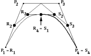
Let us use the De Casteljau’s algorithm [2, 8]. Suppose that a cubic Bezier curve, defined over the parameter interval [0, 1], is divided into two new cubic Bezier curves with corresponding parameter intervals [0, ½] and [½, 1]. Hence, the original control points P1 to P4, are used to obtain new control points

R1 to R4 and S1 to S4 for two Bezier curve segments making up the original curve. This process is illustrated in Figure 1.

Figure 1. Illustration of the De Casteljau’s algorithm

The new control points are obtained as follows:

R1 = P1,

S1 = R4,

R2 = (P1+P2)/2,

R3 = R2/2+(P2+P3)/4, (1)

S3 = (P3 + P4)/2,

S2 = (P2+P3)/4+S3/2,

R4 = (R3+S2)/2,

S4 = P4.

The subdivision can be successfully applied to split an original cubic Bezier curve at any point (the split point is on the curve) and to calculate control points for both new cubic Bezier curves.

Let us set the parameter t to any value k from the interval [0,..,k,….,1]. Suppose that C is a corresponding sub-division point of a cubic Bezier curve. According to the definition of a cubic Bezier curve (2),

B(t) = (1-t)3P1 + 3t(1-t)2P2 + 3t2(1-t)P3 + t3P4 (2) we have P1 = B(0), P4 = B(1) and C = B(k). Thus, the resulting Bezier curves are P1, R2, R3, C and C, S2, S3,

P4. Their control points, according to the corrected formula, are:

R2 =P1+ k*(P2-P1),

S3 = P3 + k* (P4-P3),

C = P2 + k*(P3-P2), (3)

R3 = R2 + k* (C-R2),

S2 = C + k*( S3`-C).

Note. A corrected formula was applied to the computational experiments [5].

2) Editing error in a formula for converting a circular arc into a Bezier arc

An arc of less than 90 degree and radius r should be considered. Assume that we have to approximate it by one segment of a cubic Bezier curve.

One approach of finding Bezier control points, when the angle of a circular arc is not included directly in the calculation of the “magic number” k,

was proposed in [5].

Let the coordinates of arc start point P1, arc end point P4 and arc center point C be (x1, y1), (x4, y4) and (xc, yc), respectively. Then:

ax = x1 – xc,

ay = y1 – yc,

bx = x4 – xc, (4)

by = y4 – yc,

q1 = ax*ax + ay*ay,

q2 = q1 + ax*bx + ay*by,

(3)

Bezier Curve

x2 = xc + ax – k2*ay,

y2 = yc + ay + k2*ax,

x3 = xc + bx + k2*by, (5)

y3 = yc + by – k2*bx.

The advantage of (5) is control points P2 and P3 refered to as world coordinates. Any rotations and transformations are not needed. For a counterclockwise arc, the value of k2 is positive, while

for a clockwise arc it is negative.

Despite the error in [5], the correctness of the proposed approach to calculate k2 and control points P2, P3 has been tested using correct formulas. The

CircuitCAM software [16] was used for testing.

3. Subdivision by

“long arc”

strategy

An algorithm to approximate an arbitrary cubic Bezier curve on the curve with a set of circular arcs is described in Section 4 of [5]. “Arbitrary” means the angle of a biarc of Bezier arc can be more than 90 degrees and a Bezier curve can have cusps, loops and inflection points.

The approximation algorithm from Section 4 of [5] can be overridden in a more compact six-step procedure:

Step 1: Subdivide the initial Bezier curve at point C where its curvature changes (convex segment changes into concave or vice versa) and take the first curve as the left Bezier curve;

otherwise take the entire Bezier curve as the

left Bezier curve.

Step 2: Subdivide the left Bezier curve in such a way

that the current Bezier curve is an initial 900

degree biarc segment; otherwise take the entire Bezier curve as a current Bezier curve.

Step 3: Approximate the current Bezier curve by a

set of circular arcs with a given error tolerance.

Step 4: If the angle of the left Bezier curve is more

than 900_{, take the remaining Bezier curve as a}

new left Bezier curve and proceed Step 2.

Step 5: If the left Bezier curve is not referred to as the

entire Bezier curve, take the remaining Bezier curve as an initial Bezier curve and go to

Step 1.

Step 6: Stop.

Obviously, Step 3 (“Approximate the current

Bezier curve by a set of circular arcs with a given error tolerance”) constitutes the core of the recursive algorithm. In [7], a curve is split at the point of maximum deviation of the spiral from the approximating biarc. The deviation is measured along a radial direction of the biarc. Five subdivision strategies (S1-S5) are proposed in [5].

All these subdivision strategies have the same basis: if the maximum deviation of the cubic Bezier curve from the approximating circular arc exceeds a given error tolerance, the Bezier curve is subdivided into two Bezier curves and the approximation algorithm is recursively used for both, new left and right Bezier curves, respectively. There are differences only in:

• calculation of the approximation arc (center point and radius of an arc);

• selection of the subdivision point (value of parameter t from the interval [0.0, 1.0]).

Two following approaches in calculating the approximation arc have been used:

A1-middle point: The approximation arc starts at Bezier start point P1, goes through Bezier “middle point” M and ends at Bezier end point P4. According to equation (1), P1 = B(0), M = B(0.5),

P4 = B(1).

A2-biarc: The approximation arc starts at Bezier start point P1, goes through the biarc joining point

G and ends at Bezier end point P4.

Three points, which are not collinear (all on the same line), uniquely define a circle. We use this definition at a circle to calculate the radius and center point of the circular arc.

The experiments showed the best results obtained by using S2 (cutting point) and S1 (middle point) strategies [5]:

S1-middle point: The subdivision point is the middle point within the interval [0, 1], i.e., t = 0.5.

S2-cutting point: The subdivision point is a point where the Bezier curve intersects the approximation arc. If intersection does not occur, then t =0.5.

The S2 better works with approach A1, while S1

showed the same results in both approaches.

The new “long arc” strategy of subdivision is

based on a simple procedure: a) set t = 0.0;

b) increase t taking interpolation step ∆t (i.e. t = t +

∆t) and subdivide temporarily the initial Bezier curve

at point t;

c) if an approximation error of the left Bezier curve is less the given error tolerance, ignore previous temporary subdivision and subdivide according to step b anew); otherwise proceed with d);

d) subdivide the initial Bezier curve at point (t -

∆t), exchange the left Bezier curve by a circular arc,

take the remaining right Bezier curve as an initial Bezier curve and repeat thr procedure from the beginning.

So, the given (t - ∆t) value gives the longest

circular arc as possible. The procedure stops, when the current initial Bezier curve can already be approximated by one circular arc with the given tolerance.

(4)

the binary search method can be used. The number of subdivisions of the Bezier curve will not exceed 10 (i.e. log21000 = 10) with the standard interpolation

step ∆t = 0.001 (one thousand points in Bezier curve).

Computational experiments have showed that decrease of the interpolation step ∆t (e.g. 0.0001 or 0.00001)

does not increase the number of resulting circular arcs.

Step 3 in details (applying the “long arc” strategy

for a subdivision):

Input: a cubic Bezier curve with increasing curvature and with angle less than 900_{, given error tolerance}_ε

and interpolation step ∆t. Output: a set of circular arcs.

1) If the current Bezier curve fits a circular arc

with given error tolerance ε, exchange the Bezier curve by one circular arc and proceed with 5).

2) Use the binary search algorithm and temporary subdivisions for the current Bezier curve to define the

smallest subdivision value t from the interval [0.0,

1.0] with step ∆t, where the left Bezier curve can not

already be approximated by one circular arc with given error tolerance ε.

3) Subdivide the current Bezier curve at point t= t - ∆t and substitute the left Bezier curve by one circular

arc.

4) Take the remaining right Bezier curve as the current Bezier curve and proceed with 1).

5) Stop.

Experimental results of the “long arc” strategy for a subdivision.

Let’s take two cubic Bezier curves from [5], shown in Figure 2. Points P1=(15.9753, 0.7421),

P2=(18.2203, 2.2238), P3=(21.0939, 2.4017) and

P4=(23.1643, 1.6148) display the first cubic Bezier curve (Example 1), points P1=(17.5415, 0.9003),

P2=(18.4778, 3.8448), P3=(22.4037, -0.9109) and

P4=(22.563, 0.7782) represent the second cubic Bezier curve (Example 2), respectively:

Example 1

Example 2

Figure 2. Cubic Bezier curves from [5]

Dots and squares on the curves show the start-end points of the resulting circular arcs.

Tables 1 and 2 show the results of approximation of the cubic Bezier curves, displayed in Figure 2, by

S1 and a new “long arc” strategy of subdivision,

respectively. Both, S1 and “long arc” strategies have

been used considering A1-middle point approach in calculation of the arc approximation.

Table 1. Results of Example 1

Error tolerance ε (mm)

Number of circular arcs

Old S1 New “long arc”

0,1 1 1

0,01 3 2

0,001 6 5

0,0001 14 10

0,00001 28 20

0,000001 57 43

Table 2. Results of Example 2

Error tolerance ε (mm)

Number of circular arcs

Old S1 New “long arc”

0,1 4 4

0,01 7 7

0,001 16 13

0,0001 32 26

0,00001 71 51

0,000001 157 110

The complexity of Step_3 with the “long arc”

strategy of subdivision is N(Mlog2M), where M=1/∆t

and N is the number of the resulting circular arcs.

4. Approximation of quadratic Bezier curves

Approximation of quadratic Bezier curves by circular arcs is quite thoroughly investigated in [1, 6, 9, 10]. Algorithms for approximation of an arbitrary quadratic Bezier curve by arc splines and experimental results are presented in [1, 6, 9, 10] as well.

The aim of this section is to adapt and test the “long arc” strategy of subdivision for approximation

of a quadratic Bezier curve.

As we can see from the description of the approximation algorithm, only the term “Bezier curve” has been used (but not a “cubic Bezier curve”). So, only three minor updates are needed in adapting and testing a proposed algorithm for approximation of quadratic Bezier curves:

1. Exchange Bezier end point P4 into Bezier end point P3 in whole text explaining the approximation algorithm.

2. In calculation of the approximation error use the quadratic Bezier formula (6) instead of cubic Bezier formula (2):

(5)

Bezier Curve

3. For subdivision of the quadratic Bezier curve use corresponding formulas to calculate new control points. Again, let us setparameter t to any value k from the interval [0,..,k,…,1]. Suppose that C is a corresponding sub-division point of the quadratic Bezier curve. Under the definition of the quadratic Bezier curve (6), we have P1 = B(0), P3 = B(1) and

C = B(k). So, the resulting quadratic Bezier curves are P1, R2, C and C, S2, P3, where their control points are:

R2 = P1+ k*(P2-P1),

S2 = P2 + k*(P3-P2), (7)

C = R2 + k*(S2-R2).

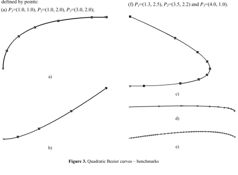
The “long arc” strategy of subdivision has been

developed and tested on the benchmarks, used in [1, 6, 9]. Five quadratic Bezier curves, shown in Figure 3, are defined by points:

(a) P1=(1.0, 1.0), P2=(1.0, 2.0), P3=(3.0, 2.0);

(b) P1=(1.0, 1.0), P2=(2.0, 1.0), P3=(4.5, 2.75); (c) P1=(1.0, 1.0), P2=(5.0, 1.0), P3=(1.0, 2.75); (d) P1=(0.54, 3.40), P2=(7.22, 3.61), P3=(7.39,

3.14);

(e) P1=(0.54, 3.38), P2=(5.61, 4.13), P3=(6.77, 3.46).

Table 3 shows the number of circular arcs, obtained when approximating the quadratic Bezier curves from Figure 3. The “long arc” strategy of

subdivision provides less arc segments for all Bezier curves.

Finally, we have compared results from five cases of the approximation test, presented in [10, 11], including results from our “long arc” strategy of

subdivision. Three benchmarks (a), (b), (c) have already been shown in Figure 3. One new quadratic Bezier curve is defined by points:

(f) P1=(1.3, 2.5), P2=(3.5, 2.2) and P3=(4.0, 1.0).

a)

b)

c)

d)

e)

Figure 3. Quadratic Bezier curves – benchmarks

Table 3. Approximation results on benchmarks of Figure 3

Benchmark tolerance Error ε (mm)

Number of circular arcs by:

Walton [6] Ahn [1] Yong [9] Our S1 Our “long

arc”

(a) 0.0005 14 10 * 8 6

(b) 0.001 8 6 * 5 4

(c) 0.001 18 15 10 12 10

(d) 0.0001 * 29 14 16 12

(e) 0.0000001 * 158 119 128 101

(6)

The obtained numerical results are presented in Table 4.

Table 4. [10, 11] and “long arc” subdivision

Bench mark

Error tolerance ε

(mm)

Number of circular arcs: Yang

[10, 11] “long arc”

(a) 0.0005 7 6

(b) 0.00001 19 18

(c) 0.001 11 10

(f) 0.001 8 5

(f) 0.0005 10 7

5. Concluding remarks

In this paper the task of approximation of the Bezier curve by as less as possible number of circular arcs is discussed. As a result, a new strategy for subdivision of a cubic Bezier curve with regard to approximation algorithm from [5] is described. This modified approximation algorithm is experimentally tested on quadratic Bezier curves as well.

The experiments showed the new “long arc”

strategy of subdivision provides much better results in comparison with the “middle point” (S1) strategy. We can see this from the empirical results presented in Tables 1 and 2.

The proposed “long arc” strategy of subdivision

can be successfully used to approximate quadratic Bezier curves. Computational experiments on widely used quadratic Bezier curves (benchmarks) showed that the best results are achieved by using the “long arc” subdivision. Empirical results are presented in

Table 3 and Table 4.

The complexity of the approximation algorithm for Bezier curve with increasing curvature by a set of circular arcs with “long arc” strategy of subdivision is

N(Mlog2M). Here M=1/∆t and N is the number of the

resulting circular arc segments.

Finally, two editing errors, made in our previous article [5], have been corrected.

Acknowledgments

The authors thank Jan Hrkal for remarks about the error in a current formula (5) from a previous paper.

References

[1] Y. J. Ahn, H. O. Kim, K. Y. Lee. G1_{arc spline} approximation of quadratic Bezier curves. Computer-Aided Design, 1998, Vol. 30, No. 8, 615−620.

[2] G. Farin. Curves and surfaces for computer aided geometric design: a practical guide. Academic Press,

1997.

[3] M. Goldapp. Approximation of circular arcs by cubic polynomials. Computer Aided Geometric Design,

1991, Vol. 8, No. 3, 227−238.

[4] H. Park. Error-bounded biarc approximation of planar curves. Comput.-Aided Design, 2004, Vol. 36, No. 12, 1241–1251.

[5] A. Riškus. Approximation of a Cubic Bezier Curve by Circular Arcs and Vice Versa. Information Technology and Control, 2006, Vol. 35, No. 4, 371−378

[6] D. J. Walton, D. S.Meek. Approximation of quadratic Bezier curves by arc splines. Journal of Computational and Applied Mathematics, 1994, Vol. 54, 107−120.

[7] D. J.Walton, D. S. Meek. Approximation of a planar cubic Bezier spiral by circular arcs. Journal of Computational and Applied Mathematics, 1996,

Vol. 75, No. 1, 47−56.

[8] F. Yamaguchi. Curves and Surfaces in Computer Aided Geometric Design. Springer Verlag, 1988.

[9] J.-H. Yong, S.-M. Hu, J.-G. Sun. Bisection algorithms for approximating quadratic Bezier curves by G1_{arc splines.} _{Computer-Aided Design}_{, 2000,} Vol. 32, No. 4, 253−260.

[10] X. Yang. Approximating NURBS curves by arc splines. In: Martin R,Wang W, editors. Proceedings of Geometric Modeling and Processing 2000, Hong Kong. Los Alamitos. IEEE Computer Society Press, 2000. pp.175−183.

[11] X. Yang. Efﬁcient circular arc interpolation based on active tolerance control. Comput-Aided Design, 2002, Vol. 34, No. 13, 1037–1046.

[12] G. Liutkus, A. Riškus, A. Tomkevičius, A. Lenkevičius. Issues with exchange of presentation data among CAD systems. Information Technology and Control, 2012, Vol. 41, No. 4, 385−391.

[13] S. H. Kim, Y. J. Ahn. An approximation of circular arcs by quartic Bezier curves. Computer- Aided Design, 2007, Vol. 39, 490−493.

[14] A. Ahmad, R. Masri, J. Ali. New Approach to Approximate Circular Arc by Quartic Bezier Curve.

Open Journal of Applied Sciences, 2012, Vol. 2,

No. 4B, 132−137.

[15] Y. J. Ahn, Y. S. Kim, Y. Shin. Approximation of circular arcs and offset curves by Bezier curves of high degree. Journal of Computational and Applied Mathematics, 2004, Vol. 167, 405–416.

[16] CircuitCAM. Available from WWW:

http://www.lpkf.com/products/rapid-pcb-prototyping/software/circuitcam-pcb/index.htm .