Digital Controllers Design For Automatic Voltage
Regulator (AVR) Using Model Order Reduction
Methods
Asst. Prof. Nasir Ahmad Al-awad
Computer Engineering Dept., Mustansiriyah University, Iraq.Date of publication (dd/mm/yyyy): 26/10/2017
Abstract – To examine compensators automatic voltage regulator (AVR), fourth order framework are very unpredictable, in examination and outline. In this paper, show arranges lessening procedure is utilized for controller plan (AVR). To start with dynamic model for controller is acquired utilizing set of conditions which gives fourth order exchange work. At that point this fourth order exchange work is lessened to First Order Process with Time Delay (FOPTD) utilizing distinctive approximations techniques. At that point the computerized controllers are intended for the decreased order model of the (AVR), utilizing diverse direct plan techniques (Deadbeat, dahlin, kalman and Internal Model (IMC) controllers). Result demonstrates that the computerized controller for lessened order show gives the very attractive reaction with the first framework. All recreated are finished by utilizing MATLAB-SIMULINK tools.
Keywords – AVR, Model Order Reduction Methods, Digital Controllers.
I.
I
NTRODUCTIONIn the course of recent years, the (AVR) have been generally utilized to control producing because of their efficiencies and expenses. Concerning the limit, application and fancied execution, an alternate level of intricacy is offered for the structure of (AVR)[1]. The administer of an (AVR) is to hold the terminal voltage extent of a synchronous generator at a predetermined level; A synchronous generator's terminal voltage is a component of the measure of excitation connected to the rotor's windings.
The operation of electric power frameworks, stack changes and unusual conditions cause changes in the recurrence and planning of energy in each zone. Such changes, bringing about changes in the measure of (voltage greatness). It can be lethal in a framework; if there is extra receptive power stack for the generator terminal voltage will drop. To beat this utilization the generator excitation control utilizing AVR. The AVR rapidly reactions in case of disturbance or change in framework load [2].
The Automatic Voltage Regulator is intended to control the voltage and responsive power stream. For the stable electrical power benefit, it is critical to build up an AVR for a synchronous generator with a high proficiency and a quick reaction [3]. It is an imperative issue for the stable electrical power administration to build up the programmed voltage controller (AVR) of the synchronous generator, The AVR framework display controlled by the
PID controller, the Genetic Algorithm and Particle Swarm Optimization calculation are connected to seek a best PID parameters so the controlled framework has a decent control execution, Hence, the utilization of PID controller in the control circle drives the exciter yield promptly and enhances dynamic reaction and additionally decreases the steady state error, in case of interruption or change in framework load[4].
Control systems, for example, PI controllers, decentralized controllers, ideal controllers and versatile controllers are received for AVR to direct the genuine and receptive power output[5]. There are numerous strategies, for example, root-locus, eigenvalues procedures, versatile control, have been utilized, however every one of these techniques, show vulnerabilities can not be considered unequivocally at the plan state so the sliding mode control is effective strategy can used[6].
(AVR) is a basic element for control framework operation. Consequently, to watch the conduct and execution of AVR, investigation of its demonstrating is fundamental. Since AVR is a mind boggling framework having higher request exchange work, so it is repetitive to examine it.[7].
To concentrate such framework, thorough arithmetic is required amid displaying and consequently controls calculations wind up plainly mind boggling. At this stage, idea of decreased request demonstrating mitigates control specialists and experts by lessening the many-sided quality of models [8, 9]. Model order reduction (MOR) fundamentally holds the most critical properties amid demonstrating while at the same time dismissing undesirable or less noteworthy parameters.
the diminishment of measurement of higher-arrange framework is a simple apparatus so the previously mentioned necessities can be met with lesser intricacy and cost since multifaceted nature of framework increments with framework arrange [12].
In literature, numerical methodologies/calculations to diminish the request of a higher-arrange framework spoke to scientifically however applications are slightest [13, 14]. Later on, these techniques have been connected on physical frameworks of substantial size. However there is a little attention to the specialists on these applications for different building applications. The majority of the current examinations of computerized AVRs have been concentrating on refined control calculations, for example, those of self tuned and versatile controllers [15]. To maintain a strategic distance from these complexities, this paper displays a compelling and clear advanced outline which can be effortlessly actualized. For displaying this strategy the AVR is spoken to by a first order with time-postpone guess and the controller configuration is done specifically in the z-space utilizing diverse computerized controllers. The total framework counting the computerized control calculation has been mimicked utilizing a product (MATLAB)
In this paper, diverse MOR plans have been connected to AVR keeping in mind the end goal to distinguish the lessened model and relative investigation has been done to choose best model for various execution measures, additionally extraordinary computerized controllers can be utilized for each diminished models to discover which one the best to fulfilled outline determinations.
II.
AVR
M
ODELINGAVR framework comprises of four (4) principle parts there are amplifier, exciter, generator and sensors. The numerical model and exchange capacities can be to straight considering the time constant and disregarding immersion or other nonlinear. There are can be appeared in Fig (1)
A) Amplifier model [1]
Amplifier models expressed by a gain with (Ka) symbol and time constant with (Ta) symbol. Transfer function is:-
)
1
...(
...
...
)
1
(
TaS
Ka
Ve
Vr
B) Exciter Model [1]
The transfer function of a modern exciter can be expressed by a gain with (Ke) symbol and single time constant with (Te) symbol, and then the transfer function is:
)
2
...(
...
...
)
1
(
TeS
Ke
Vr
Vf
C) Generator Model [1]
In a linearized form, the relationship transfer function of voltage terminal generator with voltage field can be expressed by a gain (Kg) and time constant (Tg). The transfer function is :
)
3
...(
...
...
)
1
(
TgS
Kg
Vf
Vt
D) Sensor Model [1]
Sensor is modeled with a simple first order transfer function, written by:
)
4
...(
...
...
)
1
(
TrS
Kr
Vt
Vs
Utilizing the above models results in the (AVR) block-diagram shown in fig(2) The open-loop transfer function of the block-diagram in fig(2) is:
)
1
)(
1
)(
1
)(
1
(
)
(
TrS
TgS
TeS
TaS
KaKeKgKr
s
G
After taking some typical values of the above time constants and gains, the transfer-function of the VAR is
[1]:-)
5
...(
...
)
1
2
)(
1
)(
1
1
.
0
)(
1
5
.
0
(
1
)
(
s
s
s
s
s
G
III. A
PPROXIMATEO
RDERT
RANSFERF
UNCTIONS–
F
IRSTO
RDERP
ROCESS WITHT
IME DELAY(FOPDT)
High-arrange control framework frequently contains immaterial posts that have little impact on the transient reaction. Along these lines given a high-arrange framework, it is attractive, and every now and again conceivable to discover low-arrange approximating framework, with the goal that the investigation or outline exertion is diminished, as a rule, the exchange capacity might not have the purported overwhelming shafts so it may not be evident that are posts that might be disregarded keeping in mind the end goal to land at low-arrange identical [16]. As talked about before, demonstrate lessening is a capable device that allows the precise era of cost-effective portrayals of vast scale frameworks. The moderate reaction at little circumstances (because of the littlest time constants) can be approximated with a period postpone term. Keeping just a single time steady offers ascend to a FOPDT exchange work. There are numerous approaches to lessen the request of an exchange work is inexact the little time constants with comparing time postpone terms. Here, we apply diverse MOR calculations to get the streamlined model of AVR portrayed in equ. (5). Note that, in all the connected lessening plans, we have attempted to inexact the fourth order AVR plant to the principal arrange pulse time delay model.
A) Taylor Series FOPDT
For example, if T1 > T2 > T3 > T 4 is the largest time constant, the following 4th order transfer function can be approximated with the following FOPDT model [17]:-
)
6
...(
...
...
)
1
2
(
1
)
(
6 . 1
s
e
s
GrT
s
B) Skogestad FOPD
Skogestad has proposed a related method. He suggests that the largest neglected time constant should be split between the smallest retained time constant and the time delay. So, Skogestad’s FOPDT model would be[18]:
Gr(s) =
For the system under control equ. (5), the reduced Skogestad Transfer-function becomes:-
)
7
(
)
1
5
.
2
(
1
)
(
1 . 1
s
e
s
GrS
s
C) Process Reaction Curve FOPD
First approximates the given process into first order plus dead time model using process reaction curve method as:- (i) Give the step input of magnitude ‘u’ for the given
higher order process
(ii) Obtain the process reaction (S- shaped) curve as shown in Fig (3).
(iii) From the process reaction curve find the steady state value, which equal to (1)-t1=time corresponds to 28.3% of steady-state value and t2=time corresponds to 63.2% also of steady-state value.
(iv) Approximate the first order plus dead time model using the given formulae as [19, 20]:-
)
1
(
)
(
Ts
Kpe
s
GrR
TdsWhere Kp is the process gain, (T) is the process time constant and (Td)is the process dead time.
Τd= t2- T
The approximated first order time delay model is obtained and is given by:-
) 8 ....( ... ... ) 1 943 . 2 (
1 ) (
889 . 1
s e s GrR
s
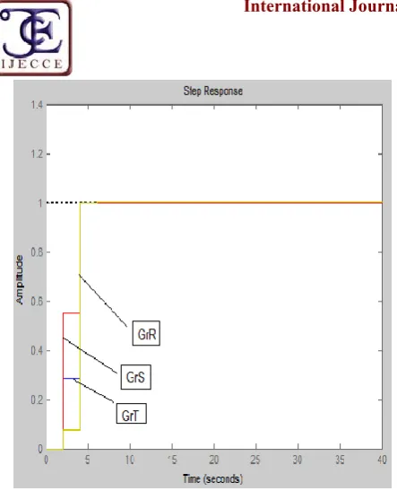
Fig (4) shows the transient response comparison between, the original system and all models reduction. Table (1) shows the transient design specifications, for all three reduced models with the original system.
Table (1) shows the transient design specifications, for all three reduced models with the original system. method Max.ove
rshoot %
Rise-time (sec)
Settling-time (sec)
Steady state error Original system 0 5.36 9.88 0 Taylor Series FOPDT 0 4.39 9.42 0 Skogestad FOPD 0 5.49 10.9 0 Process Reaction
Curve FOPD
0 6.47 13.4 0
IV.
M
ODIFIEDZ-T
RANSFORM FOR ALL THEFOPD
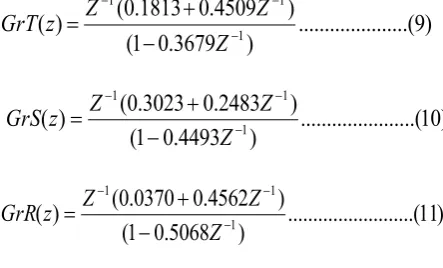
To design a digital controller the systems must first be transformed from the s-domain to the z-domain. For a system transfer functions GrT(s), GrS(s) and GrR(s) the z-domain transfer function GrT(z), GrS(z) and GrR(z) can be obtained by using modified Z-transform equation[21, 22], or directly using Mat lab for the modified Z-T for time delay model with zero-order hold device, in the above transforms, the sampling time(Ts) is chosen as (1sec).For all FOPDT, Taylor Series, Skogestad and process reaction curve, we can get the transfer functions as:-
)
9
.(
...
...
)
3679
.
0
1
(
)
4509
.
0
1813
.
0
(
)
(
11 1
Z
Z
Z
z
GrT
)
10
..(
...
...
)
4493
.
0
1
(
)
2483
.
0
3023
.
0
(
)
(
1 1 1
Z
Z
Z
z
GrS
)
11
...(
...
...
)
5068
.
0
1
(
)
4562
.
0
0370
.
0
(
)
(
11 1
Z
Z
Z
z
GrR
V. D
ESIGN OFD
ISCRETEC
ONTROLLERDigital controller can be designed directly in the z-plane or indirectly [23]. In the indirect design method an acceptable analog controller is designed first in the s-plane, and then the digital controller is found by some transformation method. This approach is especially useful when a portion of an existing control system is to be replaced, but it usually results in poorer performance than can be obtained by designing a complete digital controller directly, for this reason in this paper, the direct discrete methods can be used. (AVR) has been controlled with different types of discrete controller using the following methods: Deadbeat, Kalman’s and dahlin’s algorithms. The design specifications are:-
1. The control loop must be stable (improve the dynamic response).
2. The error should return to zero following a step load change. The deviation in the transient state must also be minimized (reduce or eliminate the steady state error).
A) Deadbeat Algorithm
The algorithm that requires the closed loop response to have finite setting time, minimum rise time and zero steady state error is referred to as a deadbeat algorithm specification that satisfies these criteria is[21, 24 ]:-
) 12 .( ... ... )
( ) ( Z K
z R
z C
of equs. (9), (10) and (11).in these equs, the delay equal one, where (
Z
1)
in numerators of these equs.This specification requires that the controlled variable shall reach the set point at t=1T i.e. after a delay of one sampling period. Substituting for C/R from above equation into all equations (9), (10) and (11), by using below equ. To find the deadbeat controller D(z):-
)
13
...(
...
1
)
(
1
)
(
1 1
Z
Z
z
G
z
D
Let take only one case to derive this controller, for Taylor Series FOPDT, GrT(z)
Substitute equ ((9) in equ (13), it get:-
1
1 1
1
( ) ...(14)
(0.1813 0.4509) 1 0.3679 1 ( ) ( ) 1 Z D z
Z Z Z
Z G z D z
z For closed-loop system
) 15 ...( ... ... 1 ) ( ) ( 1 ) ( ) ( ) ( ) ( Z z D z G z D z G z R z C
Let the unit-step input, so that the output C(k)is:-
...
)
(
kT
Z
1
Z
2
Z
3
C
The deadbeat response has the following characteristics: Zero steady-state error, minimum rise time, minimum settling time, less than 2% overshoot/undershoot and very high control signal output. The same procedures can be applied for Skogestad FOPD and Process Reaction Curve FOPD, in sometimes this method suffers from intersampling ripples. Fig (5) shows the transient response comparisons of all models with deadbeat controller. It is clear all models gives the same rise time=1.6sec and settling time=1.96sec, because, equ. (9), (10) and (11) are satisfied the same desired design equ (15).
B) Dahlins Algorithm
The Dahlin-Higham design method was popular in early digital process control design because the calculations required for the design are very simple. It is a special case of error feedback with complete cancellation [25]. The Dahlin controller is similar to the dead-beat controller in the sense that the desired closed loop transfer function equ(15) is specified, from which the discrete time controller is found using the formula given as[25, 26]:
)
16
...(
...
)
1
(
)
1
(
)
1
(
)
(
1
)
(
1 ( 1)) 1 (
N NZ
Z
Z
z
G
z
D
Let take only one case to derive this controller, for Taylor Series FOPDT, GrT(z)
Where
e
(Ts/T)
e
(2/2)
0
.
3678
, and8
.
0
Ts
Td
N
(T, Td) are the time constants and delay of all equs(6), (7)and (8). In equ. (16), let N=0, because(N) is the integral
multiples of delay-time. The same procedures, for deadbeat controller can be used equ. (15).
( ) ( ) ( ) 0.6322
( ) 1 ( ) ( ) 0.3678
C z G z D z
R z G z D z Z
The only difference is that now the desired transfer function is no longer dead-beat, but first order transfers function with a time delay. The same procedures can be applied for Skogestad FOPD and Process Reaction Curve FOPD. Fig (6) shows the transient response of all models with Dahlins controller. Table (2) shows the transient design specifications, for all three reduced models, where the Skogestad FOPD, gives better performance (low values of rise and settling times).
Table (2) shows the transient design specifications, for all three reduced models using Dahlins algorithm. Method Max.
overshoot% Rise-time (sec) Settling-time(sec) Steady state error Taylor Series FOPDT
0 4.51 7.89 0 Skogestad
FOPD
0 3.54 6.42 0 Process Reaction
Curve FOPD
0 6.53 11.6 0
C) Kalman algorithm
To synthesis a digital control algorithm by Kalmns algorithm assumes a specific C(z) and the response to a unit-step input reaches the final value in two sampling time instant and remains in it . The expression for C(z) is[26 ]:-
)
17
.(
...
1
)
(
z
C
Z
1
Z
2
Z
3
C
And, the output of digital controller is:-
)
18
.(
...
1
0
)
(
z
M
M
Z
2
MfZ
3
M
For step input
1
)
(
z
z
z
R
The closed-loop pulse transfer function is:-
)
21
...(
...
)
(
)
(
)
(
)
(
)
(
)
20
..(
...
...
)...
(
)
(
)
(
2
1
0
)
(
)
(
)
1
(
)
0
1
(
0
)
(
)
(
...)
1
0
)(
1
(
)
(
)
(
2 1 2 1 2 1 1z
Q
z
P
z
M
z
C
z
HGp
z
Q
z
R
z
M
Z
q
Z
q
q
z
R
z
M
Z
m
mf
Z
m
m
m
z
R
z
M
mfZ
Z
m
m
Z
z
R
z
M
The coefficient in HGp(z) must equal those in P(z) an Q(z), so that:-
Kp
q
q
q
qi
and
p
p
pi
i i1
2
1
0
1
2
1
2 0 2 1
So that)
22
(
...
...
)
(
1
)
(
)
(
)
(
)
(
1
)
(
)
(
z
P
z
Q
z
P
z
Q
z
P
z
P
z
D
For Taylor Series FOPDT, equ(9), to apply this steps, firstly,
Added numerator coefficient value=0.1813+0.4509=0.6322 2 1 1 1 2 1 1 1
7132
.
0
2867
.
0
1
5819
.
0
5817
.
1
)
(
1
)
(
)
(
5819
.
0
5817
.
1
7132
.
0
2867
.
0
)
(
)
(
5819
.
0
5817
.
1
7132
.
0
2867
.
0
6322
.
0
3679
.
0
6322
.
0
6322
.
0
4509
.
0
6322
.
0
1813
.
0
)
(
)
(
)
(
Z
Z
Z
z
P
z
Q
Z
D
Z
Z
Z
z
Q
z
P
Z
Z
Z
Z
z
Q
z
P
z
G
Use equ. (15), to find
2 3 2
367
.
0
262
.
0
608
.
0
286
.
0
)
(
)
(
1
)
(
)
(
)
(
)
(
Z
Z
Z
Z
z
D
z
G
z
D
z
G
z
R
z
C
The same procedures can be applied for Skogestad FOPD and Process Reaction Curve FOPD. Fig (7) shows the transient response of all models with Kalmns controller, as seen from fig, all the responses reach final value after 2-samples (2T=4sec). Table (3) shows the transient design specifications, for all three reduced models, where the Process Reaction Curve FOPD, gives better performance (low values of rise time). Kalmans controller can be considered as a modified deadbeat sense, under steps are taken to prevent excessive oscillation of the control signal.
Table (3) shows the transient design specifications, for all three reduced models using Kalman algorithm. Method Max.
overshoot% Rise-time (sec) Settling-time (sec) Steady state error Taylor Series
FOPDT 0 3.02 3.94 0
Skogestad FOPD 0 3.19 3.91 0 Process Reaction
Curve FOPD
0 1.73 3.96 0
D) IMC Algorithm
The other major single-loop controller algorithm is the IMC controller, The IMC controller, firstly is synthesize and implement by Garcia and Morari[ 27], and structure is shown in Fig(8), using the same design procedures in reference[27, 28], for Taylor Series FOPDT, The controller algorithm is an approximate inverse of the process model. The approximation is required to ensure that the controller is physically realizable. The design approach involves factoring the process model into invertible
HGm
(
z
)
and noninvertibleHGm
(
z
)
. The controller is the inverse of the invertible factor. So that, [27 ])
23
...(
...
)]
(
[
)
(
z
HGm
z
1Gcp
A filter F(z) is included in the feedback path to modulate adjustments in the manipulated variable and to increase robustness to model error.
1
1
1
)
(
Z
z
F
let inverse of the process model equ(9), which is equal to equ(23) and multiply by filter transfer function, or:-
1 1
1 1
( ) * ( ) [ ( )]
1 0.3679 (1 )
...(24)
0.1813 0.4509 (1 )
Gcp z F z HGm z Z Z Z
Take the value of (
)
as in Dahlins algorithm, and after some calculations, the closed-loop transfer function is:-3679 . 0 6321 . 0 ) ( ) ( z z R z C
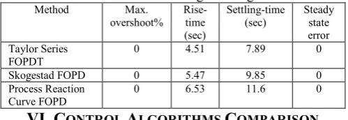
Repeat the same procedures for Skogestad FOPD and Process Reaction Curve FOPD to calculate closed-loop transfers functions. Fig (9) shows the transient response of all models with IMC controller. Table (4) shows the transient design specifications, for all three reduced models, where the Taylor FOPD, gives better performance (low values of rise and settling times).
Table (4) shows the transient design specifications, for all three reduced models using IMC algorithm. Method Max.
overshoot% Rise-time (sec)
Settling-time
(sec) Steady state error Taylor Series
FOPDT
0 4.51 7.89 0 Skogestad FOPD 0 5.47 9.85 0 Process Reaction
Curve FOPD 0 6.53 11.6 0
A definitive objective is constantly great control execution. Advanced control frameworks can execute and additionally identical ceaseless control frameworks under specific circumstances, yet they have potential troubles that ought to be considered in calculation plan. Figs (5, 6, 7, 9) demonstrates the yield of the VAR under the control of the contemplated control calculations. It demonstrates that every one of the controllers could appropriately take after the progression input. For all estimations of (K) in equ (12) and (N) in equ (16), (1-Z) factor of the denominator, demonstrating the nearness of necessary activity. Which determine zero consistent state error set-point changes. The time steady (T) fills in as an advantageous tuning parameter for the control calculation. Little estimations of (T) deliver tight control while huge estimations of (T) give more slow control. This adaptability is particularly helpful in circumstances where the parameters of the procedure demonstrate, particularly the time delay, By picking a bigger (T) and "releasing" the control activity, the controller can better suit the wrong model, As (T) approach zero, (i.e., An approach zero), Dahlin's calculation is comparable to Deadbeat calculation, however as talked about before such tight tuning is normally not attractive for AVR applications, be watchful for Deadbeat calculation intersample swell happens in the controlled variable, and the controller yield after the zero-arrange hold exchanges on either side of a steady esteem. Ringing is because of the nearness of post very near the unit hover for instance (at Z=0.8), yet for all models, equs (9, 10, 11), there is a solitary shaft at (Z=0) and the other at (Z=0.3679, 0.4493, 0.5068).The previously mentioned discourse calls attention to that the lessened models acquired can be utilized to plan controller having required trademark; let us say some part of considered power system is often subjected to unwarranted disturbances, in that case it is required that we implement controller using Deadbeat algorithm based reduced model as time response characteristics match is excellent.
VII. C
ONCLUSIONSThis paper presents different reduced order models of AVR system and the comprehensive study of their time domain characteristics. The study of reduced order models of system shows that even though the time response of some of reduced order model are emulating their original system characteristics very well, From table (1) and fig(4), it clear, the Skogestad FOPD approximates the original system. Hence using this reduced order model in controller design, one can make AVR to take right decision in event of any unwarranted disturbance in generator. Except Deadbeat algorithm, comparing these three responses reveal, that Kalman response reaches the set-point faster, because the rise and settling times are small.
Among the control algorithms, the one which performed better was the Deadbeat of first order, followed by the Kalman controller, and the third best was the Dahlin and the last one IMC. Besides having the best performance, the Deadbeat also very easy in implemented. From tables (2, 3, 4), it is clear Taylor Series FOPDT and Process
Reaction Curve FOPD, gives the same transient specifications, for Dahiln and IMC algorithms, because using the same expression
e
(Ts/T) for a first-order system.Generally, Skogestad FOPD, is the best for Kalman controller. The performance achieved with the IMC controller is equivalent to the performance achieved with a proportional-integral controller. However, the IMC design framework can readily be applied to higher-order systems.
R
EFERENCES[ 1
] Hadi Saadat, “Power system analysis”, McGraw-Hill, 1999. [2] R.Jegatheesan, “Power system operation and control, “Srm
University, EE 0403
[3] Deepak M.Sajnekar, “Comparison of Pole Placement & Pole Zero Cancellation Method for Tuning PID Controller of A Digital Excitation Control System.”International Journal of Scientific and Research Publications, Volume 3, Issue 4, April 2013.
[4] Ching-Chang Wong.”Optimal PID Controller Design for AVR System”, Tamkang Journal of Science and Engineering, Vol. 12, No. 3, 2009
[5] I Kocaarslan, E Cam.”Load frequency control in two area power systems using fuzzy logic controller”, Energy conversion and management V46, No.2, 2005
[6] M Ouassaid;”Transient stability enhancement of power system using observer-based sliding mode control”, advanced and applications in sliding mode control systems, Springer ltd, 2015. [7] Shivanagouda Biradar, “Simplified Model Identification of
Automatic Voltage Regulator Using Model-Order Reduction”, International Conference on Power and Advanced Control Engineering (ICPACE), 2015
[8] B. D. O. Anderson and Y. Liu, "Controller reduction: concept and approaches, " IEEE Transactions on Automatic Control, vol. 34, no. 8, 1989.
[9] S. Saxena and Y. V. Hote, Load frequency control in power systems via internal model control scheme and model-order reduction, IEEE Transactions on Power Systems, vol.28, no. 3, 2013.
[10] M. Vishvakarma, Y. V. Hote, and S. Saxena, "Application of model order reduction techniques: A review and future prospect”, in proc. NSI 39, 2013, Haridwar, India.
[11] G. Obinata, B. D. O Anderson, Model order reduction for control system design, Springer-Verlag, London, 2001.
[12] A.C. Antoulas, D.C. Sorensen, and S. Gugercin, "A survey of model order reduction method for large scale systems, “Contemporary mathematics, vol. 280, 2001.
[13] M.F. Hutton and B. Friedland, “Routh approximations for reducing order of linear time-invariant systems, “IEEE Transactions on Automatic Control, vol. AC-20, no. 3, June 1975.
[14] O. K. Erol and I. Eksin, “New optimization method: Big Bang– Big Crunch, “Advances in Engineering Software, vol. 37, pp. 106–11, 2006.
[15] A. Ghandakly and P. Kronegger, "Digital Controller Design Method for Synchronous Generator Excitation and Stabilizer Systems, Part I: Methodology and Computer Simulation, " IEEE Trans. on Power Systems, Vol. No. 3, 1987
[16] D K anand, R B zmood, ”Introduction to control systems”, Butterworth company, 1995
[17] Normoy Rico, “Control of dead-time processes”, Springer pub company.2007
[18] Sigurd Skogestad, “Simple analytic rules for model reduction and PID controller tuning”Modeling, Identification and control, V24, N2, 2004
[19] Seborg, D. E., Edgar, “Process Dynamics and Control”, John Wiley & Sons, Inc. 1989.
Conference on Science, Technology, Engineering & Management, V10, July 2015.
[21] M S Fadali, “Digital control engineering analysis and design”, Elsevier Inc, 2009.
[22] Kannan M. Moudgalya, “Digital Control”, John Wiley & Sons, Ltd, 2007
[23] C L Phillips, “Digital control system analysis and design”, Prentice-Hall, 1995.
[24] Sathya S, Arun jayakar S, “CONTROLLER OF PRESSURE TANK USING DEADBEAT AND KALMAN S ALGORITHM”, International Journal of Innovative Research in Technology, Science & Engineering (IJIRTSE), V1, No.10, 2015.
[25] Dahlin, E. B., ”Designing and Tuning Digital Controllers”, instrument. and Control Systems V41, No6, 1968.
[26] K.Warwick, ”Industrial digital control systems”. Peter peregrines Ltd, 1988.
[27] Carlos A. Smith, “Principles and Practice of Automatic Process Control”, John Wiley & Sons, Inc., 1997.
[28] Morari, M., and E. Zafiriou, “Robust Process Control”, Prentice-Hall, Engle wood Cliffs, NJ, 1989.
Fig. 1. General model of (AVR) [1]
Fig. 2. A simplified VAR block-diagram
Fig. 3. Open Loop Step Response of the higher order
Process For step input
Fig. 4. Shows the transient response comparison between original system and all reduced models
Fig. 5. Shows step response of all models
With Deadbeat algorithm
Fig. 7. Shows step response of all models with Kalman
algorithm
![Fig. 1. General model of (AVR) [1]](https://thumb-us.123doks.com/thumbv2/123dok_us/8785748.1763902/7.595.316.528.495.747/fig-general-model-of-avr.webp)