Open Access
Research article
Randomized trials, generalizability, and meta-analysis: Graphical
insights for binary outcomes
Stuart G Baker*
1and Barnett S Kramer
2Address: 1Biometry Research Group, Division of Cancer Prevention, National Cancer Institute, USA and 2Office of Disease Prevention, National
Institutes of Health, USA
Email: Stuart G Baker* - [email protected]; Barnett S Kramer - [email protected] * Corresponding author
Abstract
Background: Randomized trials stochastically answer the question. "What would be the effect of treatment on outcome if one turned back the clock and switched treatments in the given population?" Generalizations to other subjects are reliable only if the particular trial is performed on a random sample of the target population. By considering an unobserved binary variable, we graphically investigate how randomized trials can also stochastically answer the question, "What would be the effect of treatment on outcome in a population with a possibly different distribution of an unobserved binary baseline variable that does not interact with treatment in its effect on outcome?"
Method: For three different outcome measures, absolute difference (DIF), relative risk (RR), and odds ratio (OR), we constructed a modified BK-Plot under the assumption that treatment has the same effect on outcome if either all or no subjects had a given level of the unobserved binary variable. (A BK-Plot shows the effect of an unobserved binary covariate on a binary outcome in two treatment groups; it was originally developed to explain Simpsons's paradox.)
Results: For DIF and RR, but not OR, the BK-Plot shows that the estimated treatment effect is invariant to the fraction of subjects with an unobserved binary variable at a given level.
Conclusion: The BK-Plot provides a simple method to understand generalizability in randomized trials. Meta-analyses of randomized trials with a binary outcome that are based on DIF or RR, but not OR, will avoid bias from an unobserved covariate that does not interact with treatment in its effect on outcome.
Background
Consider a randomized trial in which subjects are rand-omized to either a control or experimental intervention. The approach to statistical inference depends on the ques-tion one would like to answer.
One question is "What would be the effect of an interven-tion on outcome if we turned the clock backwards so that
subjects randomized to the experimental treatment received the control treatment and vice versa?" Of course this question cannot be answered empirically by direct observation because one cannot go back in time. In a landmark paper on causal inference, Rubin [1] presented a stochastic answer, demonstrating that the estimated treatment effect in a randomized trial is an unbiased esti-mate of the treatment effect if the clock were turned
Published: 16 June 2003
BMC Medical Research Methodology 2003, 3:10
Received: 28 March 2003 Accepted: 16 June 2003
This article is available from: http://www.biomedcentral.com/1471-2288/3/10
backwards and the treatments were reversed. Rubin [1] noted that estimates are generalizable to a target popula-tion if the subjects in the study are a random sample from the target population. (See [2] and [3] for additional dis-cussions of the Rubin causal model including the require-ment that the effect of treatrequire-ment on one subject is independent of the effect of treatment on another subject.)
A broader question is "What is the effect of intervention in a different population that is not a random sample from the target population?" This question cannot be answered empirically. (In fact, if it were required for valid generali-zation of results, it would present a serious limitation of the scientific method in medical decision making.) In the most general situation in which the treatment effect varies by population, the question is also unanswerable stochas-tically. However a restricted version of this question can be answered stochastistically. Our starting point is to pos-tulate an unobserved baseline binary random variable. Unobserved baseline variables have often been consid-ered in discussing randomization. According to Meier [4] "...the role of randomization is to distribute the effects of baseline variables, both measured ones and those not observed, in such a way that the statistical analysis makes due allowance for them. It is precisely when there are hid-den variables which may be influential that randomiza-tion is most important." To make progress we assume no interactive effect on probability of outcome between the unobserved binary variable and treatment. This assump-tion lies at the core of our ability to generalize results of clinical trials to populations other than those from whom the original sample in the trial was drawn. For some hypo-thetical situations where the non-interaction assumption for an unmeasured variable would be violated, see [5].
Using the above framework, we address the following question, "What is the effect of intervention in a popula-tion in which a different fracpopula-tion have an unobserved binary variable that does not interact with treatment in its effect on outcome?" We investigate this question for three
common outcome measures, absolute difference (DIF),
relative risk (RR), and odds ratio (OR).
In related work, Gail et al [5] estimated the bias when one fits a model without an unobserved variable to data gen-erated from a randomized trial with an unobserved varia-ble that does not interact with treatment in its effect on outcome. For binary outcomes they found no bias with
DIF and RR but a bias with OR. However their complex
formulas provide little insight to the general health pro-fessional and do not directly address our question related to generalizability. In other related work, Anderson et al [6] also showed no bias with linear and exponential (i.e. multiplicative) models in the presence of an unobserved
variable. Although Anderson et al [6] presented a plot, related to the BK-Plot, showing the effect of a continuous unobserved variable, they did not relate the plot to generalizabilty.
Methods
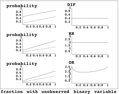
We start with a standard BK-Plot (Figure 1, left side) based on hypothetical scenarios. The BK-Plot was originally developed as a graphical approach to explain Simpson's Paradox [7,8] and extended to other problems [9]. The horizontal axis is the fraction of subjects with the unob-served baseline variable at a given level. The vertical axis is the probability of outcome, such as treatment success. The plotted lines indicate the probability of outcome as a function of the unobserved binary variable. One line cor-responds to subjects randomized to the control group, and the other line corresponds to subjects randomized to the treatment group.
We consider three common outcomes measures: the abso-lute difference in probability of outcome (DIF), the
rela-tive risk (RR), and the odds ratio (OR). Absolute
difference is derived from an additive model on the origi-nal scale; relative risk is derived from a multiplicative model on the original scale as plotted here (or an additive model on a logarithmic scale); odds ratio can be plotted on the original scale as done here, but is often derived from an additive model on a logistic scale.
For each outcome measure we present a BK-Plot under the assumption of no-interaction between treatment and the two levels of the unobserved binary variable in their effect on the outcome measure. In other words, to fulfill the condition of no interaction between the treatment and the unobserved binary variable, the outcome measure com-paring treatment groups, whether DIF, RR or OR, has the same value at the leftmost and rightmost points on the horizontal axis. As the fraction of subjects with a given level of the binary variable varies from 0 to 1, the BK-Plot traces a linear combination of the outcome measure from the leftmost to the rightmost points (Figure 1, left side).
Results
Based on Figure 1, for DIF and RR, but not OR the out-come measure was constant as the fraction of subjects with a given level varied from 0 to 1. Although the graphic is insightful, for the interested reader we provide the fol-lowing algebraic derivation of these results. Suppose the randomization groups are labeled z = treatment A or treat-ment B. Let x = 0 or 1 denote the two levels of the
unob-served binary variable. Let p denote the proportion of
subjects with the unobserved binary variable at x = 1. Let
gz(p) denote the probability of outcome in randomization
group z when a fraction p have the unobserved variable at level x = 1. Let fxz denote the probability of outcome in randomization group z when all subjects are at level x of the unobserved variable. (This represents the rightmost point of the horizontal axis in Figure 1 when x = 1). The marginal probabilities, i.e. the probabilities of outcome when a fraction p have the unobserved variable at level x
= 1, are
gA(p) = f0A(1 - p) + f1A p
Figure 1
The left side represents a standard BK-Plot, where the diagonal lines correspond to the probabilities of outcome in two rand-omization groups as a function of the fraction of subjects with the unobserved binary variable. The right side depicts a modified BK-Plot, where the outcome measure is plotted as a function of the fraction of subjects with the unobserved binary variable. We assume no interaction between the unobserved binary variable and treatment effect on the probability of outcome. Graph-ically, this means that we created BK-Plots so that the outcome measure has the same value at the leftmost and rightmost points. DIF = absolute difference; RR = relative risk; OR = odds ratio.
fraction
with
unobserved
binary
variable
0.2 0.4 0.6 0.8
1
0.2
0.4
0.6
0.8
1
probability
0.2 0.4 0.6 0.8
1
0.5
1
1.5
2
2.5
3
3.5
OR
0.2 0.4 0.6 0.8
1
0.2
0.4
0.6
0.8
1
probability
0.2 0.4 0.6 0.8
1
0.5
1
1.5
2
2.5
3
RR
0.2 0.4 0.6 0.8
1
0.2
0.4
0.6
0.8
1
probability
0.2 0.4 0.6 0.8
1
0.2
0.4
0.6
0.8
1
gB(p) = f0B(1 - p) + f1B p.
For an additive model, the outcome measure is the abso-lute difference, fxA - fxB. Under the assumption of no inter-action between treatment effect and the unobserved binary variable, fxA - fxB = DIF for x = 0, 1. This implies a constant difference in marginal probabilities, namely
gA(p) - gB (p)= DIF, which holds for all values of p.
For a multiplicative model, the outcome measure is the relative risk, fxA/fxB. Under the assumption of no interac-tion between treatment effect and the unobserved binary variable, fxA/fxB = RR for x = 0, 1. This implies a constant ratio of marginal probabilities, namely, gA(p)/gB(p) - RR, which holds for all values of p.
The results differ when the outcome measure is the odds ratio, fxA (1 - fxB)/(fxB (1 - fxA)). Under the assumption of no interaction between treatment effect and the unobserved binary variable, fxA (1 - fxB)/(fxB (1 - fxA)) - OR for x = 0, 1. However, this does not imply that gA(p) (1 - gB(p))/(gB(p) (1 - gA(p))) = OR for all p. In the Appendix we present a calculation to quantify the possible bias from using OR in a particular trial.
Discussion
There is a large literature discussing the relative merits of using RR, DIF, and OR as outcome measures [10]-[14]. Our results concerning generalizability of DIF and RR, but not OR, in the presence of an unobserved binary covariate with no interaction, add important new information to this discussion.
Because the analyst must weight all the issues, we think it is helpful to present our perspective on some of the other factors that affect the choice of outcome measure. We believe the outcome measure should reflect the underly-ing model if it is known. Also we agree that one should consider how well the model of constant RR, DIF, OR fits the data [10].
It is sometimes argued that DIF and RR should not be used because extrapolated estimates might violate the con-straints that 0 <DIF < 1 and RR > 0 [10]. (For example, suppose that in 9 trials the probability of outcome in the control group is .1 and the probability of outcome in the intervention group is .6. so DIF = .5. Also suppose that in 1 additional trial, the probability of outcome in the con-trol group is .65 and the probability of outcome in the intervention group is .95 so DIF = .3. If all trials are equal
size, a weighted estimate of DIF with weights inversely
proportional to the variance yields DIFavg = .47. The esti-mated probability of outcome in the last trial would then be .65 + DIFavg = 1.12, which violates the constraint on
DIF.) In contrast to many other investigators we are not
concerned with this extrapolation problem. In many meta-analyses the extrapolated estimates will not violate the constraints. If an extrapolated estimate violates a con-straint, it could be a valuable indication that the model is inappropriate when applied to all the studies. If the con-straint is violated only slightly, it might be sensible to fit a model that constrains DIF and RR to lie in valid ranges [11].
Sometimes it is argued that RR should not be used
because its value changes if the labels of the binary out-come are reversed [10]. In particular, if RR is constant with one set of labels it is typically not constant if the labels are reversed. However, because the labels have an important meaning (e.g. survive or die), we are not concerned that
RR changes with label reversal. In contrast, in latent class models, the class labels are arbitrary, so it is helpful to check the computations by verifying that the results are the same if the labels are reversed. A more serious criticism of RR is sensitivity to small counts [12]. We agree with this
criticism and do not recommend using RR with small
counts in one group.
We agree with much of the literature that, in terms of interpretation, RR and DIF are preferable to OR. Accord-ing to Sackett et al [14] "because very few clinicians are facile at dealing with odds and relative odds, ORs are not useful in their original form at the beside or examining room". Walter [10] writes, "The OR is undeniably the most difficult measure to intuit, so it likely to be less use-ful than RD [DIF] or RR for communicating risk"
Besides the choice of outcome measure, other factors affect the appropriateness of combining results from ran-domized trials and should be considered by the analyst. One factor is the variation in all-or-none compliance among trials. To reduce the variation from this factor, one can fit a model based on inherent compliance (i.e., with baseline subgroups "always-takers", "compliers", and "never-takers") [15,16]. These models have been applied
to meta-analyses involving DIF as an outcome [17,18].
Related models for RR [19,20] could be used for
meta-analyses involving RR. Our graphic supporting the use of
DIF and RR would directly apply to "compliers", who are the subgroup of interest in these models for all-or-none compliance.
Another factor affecting the combination of results from randomized trials is the variation in treatment (e.g. varia-tion in doses or levels of ancillary care). Despite the theo-retical results in this paper, a large empirical study
comparing the use of RR and OR in meta-analyses found
little difference in heterogeneity when using RR and OR
Publish with BioMed Central and every scientist can read your work free of charge
"BioMed Central will be the most significant development for disseminating the results of biomedical researc h in our lifetime."
Sir Paul Nurse, Cancer Research UK
Your research papers will be:
available free of charge to the entire biomedical community
peer reviewed and published immediately upon acceptance
cited in PubMed and archived on PubMed Central
yours — you keep the copyright
Submit your manuscript here:
http://www.biomedcentral.com/info/publishing_adv.asp
BioMedcentral
Conclusion
The issue of generalizability of randomized trials is impor-tant in meta-analyses of randomized trials. To avoid bias from an unobserved binary variable that does not interact with treatment in its effect on outcome (and hence increase generalizability of results), one should use DIF or
RR, but not OR, as an outcome measure.
Authors' Contributions
SGB wrote the initial draft. BSK made substantial improvements to the manuscript.
Appendix
If one has data from a randomized trial, the following
cal-culation shows the possible bias from using OR with no
interaction between treatment effect and the unobserved binary variable. Suppose the fraction of subjects with the unobserved binary variable is p = .5. From the trial we can estimate gA = gA(.5) and gB = gB(.5). With p = .5, f0z will be the same distance above gz as f1z is below gz. Therefore we can write f0A = gA(1 - s), f1A = gA (1 + s), f0B = gB (1 - k), and
f1B = gB (1 + k), where k ≤ minimum(1/gB - 1, 1) and s ≤
minimum(1/gA - 1, 1). Let OR* = gA (1 - gB)/(gB (1 - gA)) denote the apparent odds ratio. Let OR*
x = fxA (1 - fxB)/(fxB (1 - fxA)) denote the true odds ratio when all or none of the subjects have the unobserved covariate. Under the assumption of no interaction between the unobserved covariate and treatment effect, OR*0 = OR*1. Solving this equation for s gives
Substituting the above formula for s into OR*0 gives a function of k that we denote OR*0 (k). This function rep-resents possible values for the true odds ratio. For exam-ple, if gA = .2 and gB = .4, the apparent odds ratio is OR* = .375. However under the model the true odds ratio could have values OR*0(.3) = .36, OR*0(.5) = .32, or OR*0(.9) = .20.
References
1. Rubin DB: Estimating causal effects of treatments in rand-omized and nonrandrand-omized studies Journal of Educational Psychology 1974, 66:688-701.
2. Holland PW: Statistics and Causal InferenceJournal of the Ameri-can Statistical Association 1986, 81:945-960. (with discussion) to page 3. Little RJ and Rubin DB: Causal effects in clinical and
epidemio-logical studies via potential outcomes: concepts and analyti-cal approachesAnnual Review of Public Health 2000, 21:121-145. 4. Meier P: Statistics and medical experimentation Biometrics
1975, 31:511-529.
5. Gail MH, Wieand S and Piantadosi S: Biased estimates of treat-ment effect in randomized experitreat-ments with nonlinear regressions and omitted covariates Biometrika 1984, 71: 431-444.
6. Anderson S, Auquier A, Hauck WW, Oakes D, Vandele W and Weis-berg HI: Statistical Methods for Comparative Studies Tech-niques for Bias ReductionJohn Wiley & Sons, New York; 1980. 7. Wainer H: The BK-Plot: Making Simpson's paradox clear to
the massesChance15:60-62.
8. Baker SG and Kramer BS: Good for women, good for men, bad for people: Simpson's paradox and the importance of sex-specific analysis in observational studies Journal of Women's Health & Gender-Based Medicine 2001, 10:867-872.
9. Baker SG and Kramer BS: The transitive fallacy for randomized trials: If A bests B and B bests C in separate trials, is A better than C? BMC Medical Research Methodology 2002BMC Med-ical Research Methodology 2002, 2:13[http://www.biomedcentral.com/ 1471-2288/2/13].
10. Walter SD: Choice of effect measure for epidemiological data
Journal of Clinical Epidemiology 2000, 53:931-939.
11. Warn DE, Thompson SG and Spiegelhalter DJ: Bayesian random effects meta-analysis of trials with binary outcomes: meth-ods for absolute risk difference and relative risk scales Statis-tics in Medicine 2002, 21:1601-1623.
12. Olkin I: Odds ratios revisitedEvidence-Based Medicine 1998, 3:71. 13. Senn S: Odds ratios revisitedEvidence-Based Medicine 1998, 3:71. 14. Sackett DL, Deeks JJ and Altman DG: Down with odds ratios!
Evi-dence-Based Medicine 1996:164-166.
15. Baker SG and Lindeman KS: The paired availability design: A proposal for evaluating epidural analgesia during labor Statis-tics in Medicine 1994, 13:2269-2278.
16. Angrist JD, Imbens GW and Rubin DR: Identification of causal effects using instrumental variablesJournal of the American Statis-tical Association 1996, 92:444-455.
17. Baker SG and Lindeman KS: Rethinking historical controls Biosta-tistics 2001, 2:383-396.
18. Baker SG, Lindeman KS and Kramer BS: The paired availability design for historical controlsBMC Medical Research Methodology
2001, 1:9[http://www.biomedcentral.com/1471-2288/1/9].
19. Cuzick J, Edward R and Segnan N: Adjusting for non-compliance and contamination in randomized clinical trialsStatistics in Medicine 1997, 16:1017-1029.
20. Baker SG: The paired availability design: an updateIn: Nonrand-omized Comparative Clinical Studies Edited by: Abel U, Koch A. Dusseldorf: Medinform-Verlag; 1998:79-84.
21. Deeks JJ: Issues in the selection of a summary statistic for meta-analysis of clinical trials with binary outcomes.Statistics in medicine 2002:1575-1600.
Pre-publication history
The pre-publication history for this paper can be accessed here:
http://www.biomedcentral.com/1471-2288/3/10/prepub
s g g k g k k g k g g k
g k
B B A A B B
A
=1− + − −4 − + − +1 −
2
2 2 2
[ ( ) ( )