R E S E A R C H A R T I C L E
Open Access
A comparison of methods to estimate the
survivor average causal effect in the
presence of missing data: a simulation
study
Myra B. McGuinness
1,2*, Jessica Kasza
3, Amalia Karahalios
2, Robyn H. Guymer
1,4, Robert P. Finger
5and
Julie A. Simpson
2,6Abstract
Background:Attrition due to death and non-attendance are common sources of bias in studies of age-related diseases. A simulation study is presented to compare two methods for estimating the survivor average causal effect (SACE) of a binary exposure (sex-specific dietary iron intake) on a binary outcome (age-related macular degeneration, AMD) in this setting.
Methods:A dataset of 10,000 participants was simulated 1200 times under each scenario with outcome data missing dependent on measured and unmeasured covariates and survival. Scenarios differed by the magnitude and direction of effect of an unmeasured confounder on both survival and the outcome, and whether participants who died following a protective exposure would also die if they had not received the exposure (validity of the monotonicity assumption). The performance of a marginal structural model (MSM, weighting for exposure, survival and missing data) was compared to a sensitivity approach for estimating the SACE. As an illustrative example, the SACE of iron intake on AMD was estimated using data from 39,918 participants of the Melbourne Collaborative Cohort Study.
Results:The MSM approach tended to underestimate the true magnitude of effect when the unmeasured confounder had opposing directions of effect on survival and the outcome. Overestimation was observed when the unmeasured confounder had the same direction of effect on survival and the outcome. Violation of the monotonicity assumption did not increase bias. The estimates were similar between the MSM approach and the sensitivity approach assessed at the sensitivity parameter of 1 (assuming no survival bias). In the illustrative example, high iron intake was found to be protective of AMD (adjusted OR 0.57, 95% CI 0.40–0.82) using complete case analysis via traditional logistic regression. The adjusted SACE odds ratio did not differ substantially from the complete case estimate, ranging from 0.54 to 0.58 for each of the SACE methods.
Conclusions:On average, MSMs with weighting for exposure, missing data and survival produced biased estimates of the SACE in the presence of an unmeasured survival-outcome confounder. The direction and magnitude of effect of unmeasured survival-outcome confounders should be considered when assessing exposure-outcome associations in the presence of attrition due to death.
Keywords:Causal inference, Death, Iron, Macular degeneration, Missing data, Principal stratification, Sensitivity analysis, Simulation study, Survival bias, Unmeasured confounding
© The Author(s). 2019Open AccessThis article is distributed under the terms of the Creative Commons Attribution 4.0 International License (http://creativecommons.org/licenses/by/4.0/), which permits unrestricted use, distribution, and reproduction in any medium, provided you give appropriate credit to the original author(s) and the source, provide a link to the Creative Commons license, and indicate if changes were made. The Creative Commons Public Domain Dedication waiver (http://creativecommons.org/publicdomain/zero/1.0/) applies to the data made available in this article, unless otherwise stated. * Correspondence:[email protected]
1
Centre for Eye Research Australia, Royal Victorian Eye and Ear Hospital, Melbourne, Australia
Background
Attrition due to death and loss to follow-up are two major potential sources of bias in observational studies which investigate diseases of ageing. Statistical methods have been proposed to estimate exposure-outcome ef-fects in the presence of each attrition scenario separ-ately, however little is known about how the methods compare when both sources of attrition are present.
As an illustrative example, we examine the causal ef-fect of dietary iron intake on age-related macular degen-eration (AMD). Intracellular iron has been implicated in the pathogenesis of several chronic diseases of ageing, including AMD [1–3]. AMD is a chronic eye disorder responsible for severe and irreversible visual impairment in older adults. Despite evidence of elevated levels of iron in the retinal tissue of individuals with AMD, there is little evidence to suggest a link between dietary iron intake levels and the development of AMD [4].
As observed when investigating associations between other lifestyle factors and AMD, quantification of the effect of iron intake on AMD is susceptible to survival bias [5]. Individuals at risk of AMD also face the competing risk of death, and loss to follow-up is also common among elderly cohorts for whom ill-health and poor mobility can hinder attendance at study visits. When survival is associated with the exposure of interest and only participants who survive until the outcome wave are included in an analysis, expos-ure groups may lose exchangeability. Exchangeability im-plies that, conditional on the observed characteristics of individuals, an estimate of the causal relationship between the exposure and the outcome can be obtained. That is, balance of confounding variables is achieved across each category of the exposure. A loss of exchangeability can occur when there are shared predictors of survival and the outcome; in this case bias may be observed regardless of statistical adjustment for all direct exposure-outcome confounders.
The survivor average causal effect (SACE) has been pro-posed as a parameter to assess exposure-outcome rela-tionships in analyses that are susceptible to survival bias. The SACE exists within the potential outcomes frame-work, which requires us to consider all participants’ po-tential outcomes under each level of the exposure, and uses principal strata categorising the potential survival of each subject under each level of exposure to define the relevant causal effect [6]. The SACE is a measure of the average causal effect of the exposure on the outcome among participants who would survive regardless of their exposure status, commonly referred to as always-survivors [7]. Over the last two decades several methods have been developed to estimate the SACE, each requiring various assumptions to ensure identifiability [7–10].
Marginal structural models (MSMs) have been employed by several authors to estimate causal effects (including the
SACE) and have been extended to account for participants with missing outcome data due to non-attendance [11–15]. Shardell and co-authors have shown that inverse probability weighting for survival can produce unbiased estimates for the SACE when survival has been correctly modelled and there are no unmeasured survival-outcome confounders [13]. Another MSM approach proposed by Tchetgen Tchetgen involves weighting for the probability of being an always-survivor [14]. Other methods to estimate the SACE make assumptions regarding the potential outcomes of sur-viving participants, including those with missing outcome data, without explicitly modelling the distribution of miss-ing outcome data. For these methods, missmiss-ing outcome data for surviving participants are considered to be missing at random and potential outcomes can be generated for all baseline participants regardless of their attendance at the follow-up [16]. An example of this is a sensitivity analysis approach proposed by Egleston and co-authors [17].
In this paper we present a simulation study to compare the performance of two methods employed to estimate the SACE in the presence of missing binary outcome data due to death and loss to follow-up. One method involves a MSM (employing inverse probability weights for expos-ure, survival and loss to follow-up) and the other method employs the sensitivity analysis approach described above. These approaches have been chosen as they have previ-ously been demonstrated in studies with binary outcomes.
As an illustrative example we use data from the Mel-bourne Collaborative Cohort Study to estimate the associ-ation between iron intake (for simplicity expressed as binary exposure measured at baseline; low vs high sex-specific iron intake) and the presence of the late stage of AMD at a follow-up study wave.
Methods
Notation and framework for potential outcomes
For each participant, i, let an indicator of the observed exposure at baseline,Ai, equal 0 for low iron intake and 1
for high iron intake. LetZi= 1 if participantiis alive at the
start of the follow-up wave, andZi= 0 otherwise. Let the
outcome,Yi, equal 1 in the presence of AMD at the
follow-up wave and 0 otherwise. For participants who have died before the start of the follow-up wave,Yiis undefined.Riis
an indicator of attendance at the follow-up wave for participanti; again it is undefined for participants who die before that wave. Participant characteristics, (such as age and sex, represented by the vectorV) are collected at base-line. Ui is an indicator of a genotype which is associated
with both general health (and, therefore, survival) and the outcome, AMD. In the simulation study below Ui
repre-sents an unmeasured variable. Di is an indicator for
unmeasured variable. There areNparticipants at the base-line wave withnA= 0participants observed to have low iron intake,nA= 1participants observed to have high iron intake (N=nA= 0+nA= 1).nZ= 1participants are observed to sur-vive until the follow-up study wave.
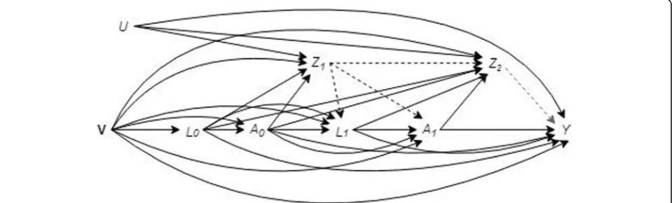
As seen in the causal diagram presented in Fig.1a, sur-vival (Z) is a collider variable on the pathway between the exposure (A) and the outcome (Y) since it is a“child”of the exposure and genotype (U) [18]. Participant inclusion in the analysis is dependent on survival until the follow-up wave. Conditioning on survival unblocks the backdoor pathway between the exposure and the outcome throughU (as seen in Fig.1b) which introduces confounding bias [19]. Under the framework of potential outcomes we can con-sider an individual’s outcomes if we were to set the expos-ure (iron intake) toa, where a can take on the values 0 (low iron intake) or 1 (high iron intake) [6]. When the value of the potential exposure for individuali(ai) is
con-trary to their observed exposure (Ai) the potential outcome
under that potential exposure is often referred to as the counterfactual outcome [20].Zi(a) is the potential survival
status andYi(a) is the potential AMD status for participant
iwhen iron intake is set toa.
Principal stratification refers to categorization of in-dividuals according to their potential survival outcome for each level of iron intake [21]. The first stratum consists of always-survivors, the individuals who are the most robust and will be alive at follow-up regard-less of iron intake level (Zi(a= 0) =Zi(a= 1) = 1). The
next stratum is comprised of never-survivors, those who are the most fragile and will not survive irre-spective of exposure level (Zi(a= 0) =Zi(a= 1) = 0).
Compliant-survivors will survive only if they have high iron intake (Zi(a= 0) = 0, Zi(a= 1) = 1), whereas
defiant-survivors will survive only if they have low iron intake (Zi(a= 0) = 1, Zi(a= 1) = 0).
Principal stratum does not change after a partici-pant has been exposed and therefore is considered to be a pre-exposure variable. A person’s principal stratum will depend on complex interactions between genetics, past behaviour and environmental factors, many of which are unlikely to be measureable. In the simulation study below, these factors are represented by the variable U which is also a predictor of the out-come. Predictors of survival determine which partici-pants are compliant-survivors. After conditioning on survival (by including data from surviving participants only), the distribution of these variables become un-balanced between principal strata and, therefore, ex-posure groups; surviving participants with higher levels of the exposure, iron intake, (who include always-survivors and compliant-survivors) will have differing levels of U compared to surviving partici-pants with lower levels of iron intake (who are all always-survivors). To obtain an unbiased estimate of the exposure-outcome effect, predictors of the out-come which are not evenly distributed between ex-posure groups (high vs low iron intake) must be accounted for in the analysis. However, traditional statistical methods cannot adjust for variables, such as U, that have not been measured. Therefore, survival bias exists when confounding of the relationship be-tween exposure (iron intake) and the outcome (AMD) by U is induced after conditioning on survival.
One assumption commonly required to identify the SACE is monotonicity. The monotonicity assumption states that iron intake will have a non-negative effect on survival. That is, participants who survive with low
Fig. 1Causal diagram for the effect of iron intake on age-related macular degeneration. V represents the vector of participant demographics (e.g. age and sex) recorded at baseline. Exposure,A, is also recorded at baseline.Zis an indicator of survival until the start of the follow-up wave.Ris an indicator of attendance at the follow-up study wave when outcome (Y, age-related macular degeneration) was ascertained. An indicator genotype,
iron intake will also survive with high iron intake, and participants who die with high iron intake will not survive with low iron intake (Zi(a= 0)≤Zi(a= 1)).
Under the assumption of monotonicity, there will be no defiant-survivors. Survivors who have low iron in-take must be always-survivors; whereas survivors with high iron intake could be either always-survivors or compliant-survivors (as seen in Fig. 2). Consequently, individuals with low iron intake are not directly com-parable to (or exchangeable with) those with high iron intake at the outcome study wave.
The survivor average causal effect (SACE)
Under the assumption of no unmeasured confounders between the exposure and outcome (sometimes re-ferred to as the strong ignorability assumption) and the assumption that principal stratum is a pre-exposure variable, the exposure groups will be exchangeable when analyses are restricted to the stratum of always-survivors [22]. Hence, there is no survival bias when assessing the association between the exposure (iron in-take) and the outcome (AMD) among this subgroup of participants. Therefore, the SACE odds ratio (SACEOR)
is defined as the ratio of the odds of AMD when a= 1
(high iron intake) to the odds of AMD whena= 0 (low-iron intake) among always-survivors (AS):
SACEOR¼odds½Y að ¼1Þ ¼1jAS
odds½Yða¼0Þ ¼1jAS ð1Þ
However, as seen in Fig.2, it is not possible to identify which participants are always-survivors without add-itional assumptions such as those described below.
The SACE is a marginal effect, meaning that it aims to reflect the effect of an exposure on an outcome averaged over the levels of unmeasured confounders within a speci-fied population. This is in contrast to the conditional odds ratio estimated via traditional logistic regression with co-variate adjustment. The conditional odds ratio will coin-cide with the SACE when there is no survival bias and the covariates do not modify the effect of the exposure on sur-vival. However, it should be noted that, unlike mean dif-ferences, risk differences or risk ratios, odds ratios are non-collapsible, meaning that the unadjusted odds ratio for the entire sample cannot be expressed as a weighted average of odds ratios from each observed pattern of con-founders. Therefore, when estimating odds ratios, condi-tional effects may differ from marginal effects even in the absence of confounding [23].
Always-survivor
Compliant-survivor
High iron intake
Survives
Never-survivor
Defiant-survivor
High iron intake
Dies
Always-survivor
Defiant-survivor
Low iron intake
Survives
Never-survivor
Compliant-survivor
Low iron intake
Dies
Estimation of the survivor average causal effect
Many approaches have been proposed to estimate the SACE [24–29]. The approaches under comparison in this study are described below. Example statistical com-puting code for estimating the SACE via these methods in Stata is available in the Additional file 1. The ap-proaches presented below require the assumption that the outcome data are missing conditional on measured covariates, and that missingness is independent of the outcome [30]. In addition, each of the methods invoke the stable unit treatment value assumption, which states that the outcome of one participant is not dependent on the exposure of another, and that there is only one ver-sion of the exposure (i.e. the level of exposure is the same for everyone who has been categorised as having high iron intake) [31]. It is also assumed that it is pos-sible for participants to have been exposed to either ex-posure level (i.e. low and high iron intake) for every observed pattern of exposure-outcome confounders; this is known as the positivity assumption [32].
Estimating marginal structural models (MSMs) with standardised weights for survival
This approach is similar to that presented by Shardell and co-authors in 2015 [13]. It uses stabilised inverse probabil-ity of observed exposure weights to achieve balance of measured baseline covariates across exposure groups.
The analysis of the exposure-outcome association is conducted via weighted logistic regression, whereby each participant,i, is weighted by an estimate ofWi:
Wi¼ A SFA¼Ai
ipiþð1−AiÞð1−piÞ
ð Þqimi ð2Þ
wherei= 1, 2,…,NandAi= 0, 1. Here,piis the propen-sity for having high iron intake for the i th participant (Eq. 3). The propensity is estimated via logistic regres-sion adjusted for all measured exposure-outcome con-founders and strong predictors of the outcome, represented by the vectorP[33]:.
Pr½Ai¼1jP¼Pi ¼pi ð3Þ
qiis the propensity for survival until the follow-up study
wave for theithparticipant (Eq.4). It is estimated via lo-gistic regression adjusted for the exposure (iron intake), all measured survival-outcome (AMD) confounders and strong predictors of the outcome. These covariates are represented here by the vector Q. Because U represents an unmeasured variable, it cannot be included as a covari-ate when estimating the probability of survival:
Pr½Zi¼1jA¼Ai;Q¼Qi ¼qi; ð4Þ
mi is the propensity for attendance at the follow-up
wave among the participants who survive (Eq. 5). This
propensity is estimated via logistic regression adjusting for iron intake, all measured attendance-outcome con-founders and strong predictors of the outcome. These covariates are denoted by the vectorM. Information on area of residence is unmeasured and thereforeD is not included as a model covariate in this example:
Pr½Ri¼1jZi¼1;A¼Ai;M¼Mi ¼mi; ð5Þ
SFAis a stabilising factor used to improve the efficiency of the weights (Eq.6) [11]. Here, it is the average of the propensity for each exposure level. Separate constant values are used as stabilising factors for participants ob-served to have low iron intake (SFA= 0) and participants observed to have high iron intake (SFA= 1) [34].
SFA¼n 1 A¼Ai
X nA¼Ai
i¼1
pi !
ð6Þ
Wi is undefined for participants who do not survive
until the follow-up study wave because non-missing out-come status can only be defined for survivors. As with any method which utilises propensity scores, the balance of covariates across exposure groups should be assessed before and after applying weights [33].
Finally a weighted logistic regression is fitted to the binary outcome (Y) with the covariates, the exposure variable (A) and baseline confounders (V). In the pres-ence of stabilised inverse probability weights, further ad-justment for baseline confounders of the exposuoutcome relationship in the final weighted logistic re-gression can reduce bias [35]. The rere-gression coefficient for the exposure is taken as the estimate of the log-odds of the SACE for this approach.
By incorporating the probability of attendance at the follow-up wave in the weight, participants with observed outcomes represent those with similar characteristics who were lost to follow-up. Weighting for survival plays a simi-lar role; the surviving participants with the lowest propen-sity for survival are given more weight to represent those participants with similar characteristics who have died.
Estimation for sensitivity analysis approach
τ¼odds½Y að ¼1Þ ¼1jCS
odds½Y að ¼1Þ ¼1jAS ð7Þ
As indicated in the original paper, τis a marginal value and it is assumed to be constant over all values of the base-line covariates [17]. If individuals with higher values of U are less likely to survive and have a higher probability of AMD then it is assumed that always-survivors will be more robust and less likely to develop AMD than those who are compliant-survivors. In this scenario, the value ofτwill be greater than one. However, if higher values ofUare associ-ated with a lower probability of both survival and AMD, then the value ofτwill be less than one. Likewise, whenU is associated with a higher probability of both survival and AMD, the value ofτwill also be less than one.
As described in the 2007 paper, whenτis not equal to one theSACEORis equivalent to [17]:.
SACEORðτ≠1Þ ¼ðν0þξ1Þðτ−1Þ−τν1þq ν0−ξ1
ð Þðτ−1Þ þτν1−q
ν0−ξ0
ξ0
whereq¼
ffiffiffiffiffiffiffiffiffiffiffiffiffiffiffiffiffiffiffiffiffiffiffiffiffiffiffiffiffiffiffiffiffiffiffiffiffiffiffiffiffiffiffiffiffiffiffiffiffiffiffiffiffiffiffiffiffiffiffiffiffiffiffiffiffiffiffiffiffiffiffiffiffiffiffiffiffi
ν0þξ1
ð Þð1−τÞ þτν1
f g2þ
4ξ1ν0ðτ−1Þ
q
ð8Þ
Here, νais the marginal probability of survival andξa
is the marginal probability of both surviving and having AMD when iron intake has been set to a. As the value of τ is not identifiable from the data, a sensitivity ana-lysis can be conducted over a range of values forτ. Con-tent matter experts must decide which values of τ are plausible in the context of the analysis.
To estimate the value ofξa, the predicted probability of
the outcome must first be estimated via covariate adjusted logistic regression, separately for participants observed to haveA= 0 (low iron intake) and for participants observed to have A= 1 (high iron intake). All measured predictors of AMD are included as covariates. The coefficients from these models are then used to predict the probability of AMD, hi(a), for all surviving participants (regardless of
missing outcome data status) under both observed and counterfactual levels of the exposure:
Pr Y½ ið Þ ¼a 1jV ¼Vi;Zi¼1 ¼hið Þa
wherei¼1;2;…;nZ¼1anda¼0;1 ð9Þ
The adjusted potential probability of survival under each exposure,gi(a), is also estimated for each participant:
Pr Z½ ið Þ ¼a 1jQ¼Qi ¼gið Þa
wherei¼1;2;…;Nanda¼0;1 ð10Þ
Under each potential exposure level, the predicted probability of AMD (hi(a), Eq. 9) is multiplied by the
predicted probability of survival (gi(a), Eq. 10) for each
surviving participant. The average is then taken as the
estimate for ξ(a= 0) or ξ(a= 1), i.e. the marginal prob-ability of surviving and having AMD under low or high iron intake, respectively:
ξa¼n1 Z¼1
XnZ¼1
i¼1
gið Þa hið Þa
wherei¼1;2;…;nZ¼1anda¼0;1
ð11Þ
Under the assumption of monotonicity, when τ is equal to 1 theSACEORis equivalent to:
SACEORðτ¼1Þ ¼ξ0ξ1ððν1−ξ1ν0−ξ0ÞÞ ð12Þ
The proof for this equation is given in the Additional file 1. Note that, under monotonicity, whenτ= 1 the distribu-tion of the outcome is equal between always- and compliant-survivors, and no survival bias is thought to be present. However, the marginal estimate derived from Eq. 12may be different to the traditional conditional estimate if measured covariates modify the effect of the exposure on survival [36].
Simulation study Data generation
A dataset of 10,000 individuals was generated to allow substantial proportions of death and missing data while still observing a relatively rare outcome within sub-groups of participants. Full details of the data generation process including model parameters and a flowchart are provided in the Additional file1.
Binary variables for sex (V1), genotype (U) and location of residence (D) were generated randomly. Mean-centred age (V2) was generated under a uniform distribution. The exposure of interest, a binary indicator of iron intake (A), was then generated conditional on sex and age. The pro-pensity for survival was generated conditional on the ex-posure, sex, age and genotype. The value of the coefficient for genotype varied between scenarios (αUZ= ln(0.5) or
ln(2)). This propensity was then used to generate a binary indicator for survival under potential exposure to high iron intake (Z(a= 1)) for every participant. For scenarios generated to be compliant with the monotonicity assump-tion, potential survival under low iron intake (Z(a= 0)) was generated among those who would survive under high iron intake (i.e. for those withZi(a= 1) = 1). For scenarios
generated in violation of the monotonicity assumption, Z(a= 0) was generated for all participants regardless of the value ofZi(a= 1). Survival status (Z) was then assigned
deterministically according to exposure (Ai) and potential
survival outcome Zi(a=Ai). Principal strata (created due
Potential outcome variables were generated for each ex-posure level (Y(a= 0) for low iron intake andY(a= 1) for high iron intake) dependent on sex, age and genotype for participants who would survive under that exposure level. The value of the coefficients for genotype (βUY= ln(0.5),
ln(1) or ln(2)) varied between scenarios. Because survival (and therefore principal strata) is also dependent on geno-type, the distribution of the outcome will differ between always-survivors and compliant-survivors. The marginal odds ratio for the difference betweenY(a= 1) andY(a= 0) was set to 0.6. This is the true value of the SACE and was chosen to reflect the estimated direction and magnitude of effect of iron on AMD in the illustrative example.
An indicator of attendance at follow-up (R) was gener-ated conditional on V1, V2, A and D among surviving participants (i.e. whenZ= 1).
The observed value ofY(AMD) was then assigned the value of Y(a= 0) or Y(a= 1) deterministically depending on the allocated exposure (A= 0 or A= 1 respectively), survival status (Z) and attendance status (R). A total of 1200 datasets were generated for each scenario. The combinations of parameters for each of the 12 scenarios are given in of the Additional file1: Table S2 .
Simulation study analysis methods
Four estimates were recorded for each of the generated datasets: (1) the log-odds of the SACE estimated via a MSM using standardised inverse probability weights for the probability of observed exposure, survival and non-attendance; the sensitivity analysis approach, (2) evaluated using a sensitivity parameter of 1 (Eq.12); (3) a sensitivity parameter of 0.5 and (4) a sensitivity parameter of 2 (Eq.8). The SACE and value of τ were estimated for each dataset using the known values of the potential out-comes (Y(a= 0) and Y(a= 1)) and principal strata. The empirical value of these parameters for each scenario was then determined by averaging the estimates derived from the 1200 generated datasets.
The absolute bias for each method was calculated within each scenario as the difference between the true SACE (odds ratio = 0.6) and the average parameter estimate (on the log-odds ratio scale) calculated across 1200 simulated datasets. The empirical standard error for each method was calculated as the standard deviation of the estimates from all simulations in each scenario [37]. To assess accuracy, the absolute bias and the empirical standard error were used to calculate the mean square error (MSE) for each es-timation method under each scenario. Standardised bias was calculated as a percentage of the absolute bias relative to the empirical standard error. Bias-corrected 95% confi-dence intervals were generated via 1000 bootstrap samples for the MSM estimate of each dataset generated and cover-age was estimated as the percentcover-age of datasets in which
the confidence interval included the true value of the SACE within each scenario [38].
Example dataset
The Melbourne Collaborative Cohort Study is a prospect-ive community-based study of 41,514 people living in Melbourne, Australia. Details of the study have been pub-lished elsewhere [39, 40]. In brief, participants attended baseline clinics (1990–1994) where information on demo-graphics, lifestyle and diet was collected. Colour digital fundus photography was performed a median of 11.8 years after baseline attendance, between 2003 and 2007.
The study protocol was approved by the Human Re-search and Ethics Committees of The Cancer Council Victoria and the Royal Victorian Eye and Ear Hospital, and was conducted in accordance with the Declaration of Helsinki. Written informed consent was obtained from all participants after explanation of the nature of the study.
Iron intake over the year prior to attendance at the base-line study wave was estimated using a 121-item food fre-quency questionnaire. Iron content in food and beverages (excluding supplements) was derived from Australian food composition tables (NUTTAB 1995) [41]. Participants were considered to have high iron intake if their intake was above the median for their sex. Participants with iron intake below the 1st and above the 99th sex-specific cen-tiles of the baseline population were considered to have potential measurement error and were excluded.
Sex, age, country of birth, smoking status, education, and recreational physical activity were recorded at the baseline wave. Education was categorised as less than technical or high school, completed technical or high school, or completed a trade or tertiary degree or diploma. Smoking status was categorised as never-smoker, former-smoker, currently smoking 1–14 cigarettes per day and currently smoking 15 or more cigarettes per day at the time of the baseline exam. Country of birth was dichoto-mised into Northern European descent (Australia, New Zealand, England, Ireland, Scotland, Wales or Latvia) and Southern European Descent (Italy, Greece or Malta). Rec-reational physical activity during the 6 months prior to the baseline exam was categorised into quartile groupings.
Late AMD was defined as the presence of choroidal neo-vascularization or geographic atrophy in either eye [42]. If only one eye was graded, that participant was omitted from the analysis, unless late AMD was detected in that eye.
at the start of the follow-up wave were excluded from this analysis.
Covariate balance was assessed among participants with non-missing outcome data before and after apply-ing MSM weights by calculatapply-ing the standardised differ-ence between high and low iron take groupings [33]. Bias-corrected 95% confidence intervals were generated via 1500 bootstrap samples for each of the estimates [38]. Because it is assumed that the unmeasured con-founders will have an opposing net effect on the prob-ability of survival and the probprob-ability of AMD (i.e. variables that decrease the probability of survival will in-crease the probability of AMD), the sensitivity analysis was restricted to values of the sensitivity parameter equal to or greater than one.
Data generation and all statistical analyses were per-formed using Stata/SE version 14.2 (StataCorp LP, Col-lege Station, TX, USA) [43].
Results
Simulation study results
A total of 12 scenarios and 14,400 datasets were analysed.
Covariate balance
The predictors of exposure, sex and age, were unbalanced between iron intake levels (average standardised difference
≥21% and≥26% for each scenario, respectively) for attend-ing survivors, as seen in Additional file1: Table S2. Balance was achieved after applying the MSM weight. However, a small difference after weighting remained among scenarios which were compliant with the monotonicity assumption (≤2.2% and≤3.0%, respectively). Location of residence was a predictor of missingness (but not exposure) and was well balanced between iron intake levels across scenarios before and after weighting (≤0.8%). The distribution of genotype was not balanced across iron intake levels despite the ex-posure being generated independently of genotype. This imbalance was largest for scenarios generated with a nega-tive effect of genotype on both survival and outcome (i.e., whenORUZ=ORUY= 0.50) and no violation of the
mono-tonicity assumption. The standardised difference for geno-type between exposure levels increased after applying the MSM weight for the majority of scenarios.
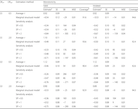
Empirical value ofτ
The empirical value ofτ(i.e. the ratio of the odds of AMD among the compliant-survivors to the odds of AMD among the always-survivors whenais set to one) was in-fluenced by the values ofαUZandβUYand varied
accord-ing to random samplaccord-ing between simulated datasets. The presence of defiant-survivors (in scenarios with vio-lation of the monotonicity assumption) did not alter the value of τ which describes the difference in outcome
distribution between always-survivors and compliant-survivors only.
In scenarios with a null effect of the unmeasured vari-able (U) on the outcome (meaning there is no survival bias), the average value ofτwas 1.00 (see Additional file 1: Table S3).
Across the remaining scenarios the average value ofτ ranged between 0.89 and 1.12 (see Table 1) and were much less extreme than the sensitivity parameters of 0.5 and 2 chosen as proxies forτwhen estimating the SACE via the sensitivity approach. Hence, the MSM estimates were more accurate than the sensitivity approach assessed at sensitivity parameters other than one in all scenarios (see Fig.3).
Bias
Survival bias does not exist in the absence of an unmeas-ured confounder which acts as a shared predictor of sur-vival and the outcome. When genotype was a predictor of survival but not the outcome, the estimated magni-tude of bias was ≤0.005 (on the log odd ratio scale) for the MSM and≤0.015 for the sensitivity analysis assessed at a sensitivity parameter of 1 (see Additional file 1: Table S3 and Figure S2).
For scenarios with an opposing direction of effect of genotype between survival and outcome, true value of τ was greater than one, meaning that always-survivors with high iron intake had lower odds of AMD than compliant-survivors with high iron intake. When it was assumed in the statistical analysis that there was no difference in out-come between principal strata (i.e. when the sensitivity parameter was set to 1 or the MSM approach was employed) the estimated effect of high iron intake com-pared to low iron intake among always-survivors was therefore diluted towards the null and the true value of the SACE was underestimated (bias≤0.042 and≤0.054 for sensitivity analysis and MSM respectively).
For scenarios with the same direction of effect of genotype between survival and outcome, the true value of τ was less than one. In these scenarios, the always-survivors with high iron intake had greater odds of AMD than compliant-survivors with high iron intake. Therefore, when the odds of the outcome was assumed to be equal between principal strata in the analysis, the true effect of the exposure on the outcome amongst always-survivors was overestimated (magnitude of bias
≤0.028 and≤0.033 for the sensitivity approach assessed at the sensitivity parameter of 1 and for the MSM ap-proach, respectively).
created with a violation of monotonicity and explains why bias was lower among these scenarios.
Distribution of estimates
The standard error was fairly consistent across estima-tion methods and scenarios, although standard errors were slightly greater, on average, for scenarios generated under the monotonicity assumption compared to sce-narios with a violation of the monotonicity assumption. Among scenarios with a non-null effect of genotype on the outcome, the majority of estimates had high values of standardised bias due to the relatively small value of the standard error compared to the absolute bias and coverage was lower than the nominal 95% confidence interval for the MSM estimates (Table1).
Results from example dataset Participants, survival and outcome
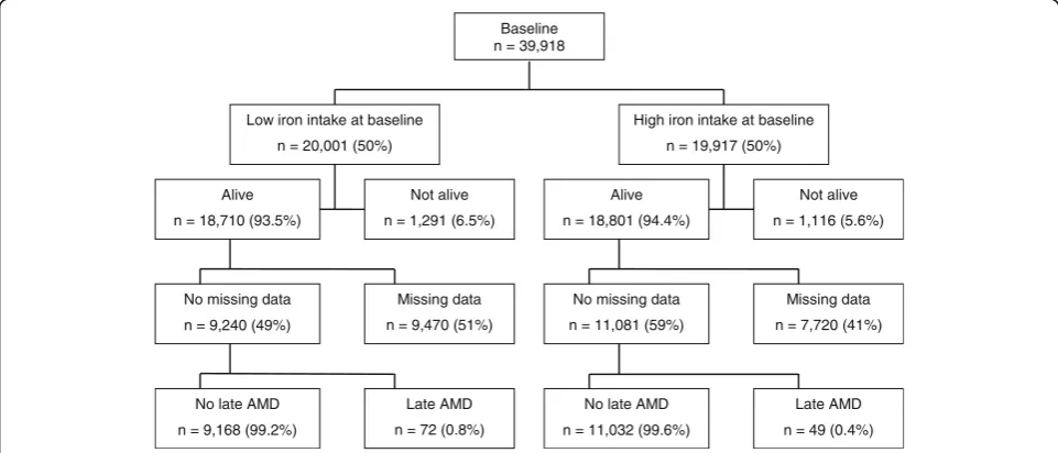
Of the 39,918 participants recruited at baseline with complete data on the exposure and potential confounders, 37,511 (94%) survived until the start of the follow-up wave. Of those 20,321 (54%) had complete data on the outcome at the follow-up wave (Fig.4). The covariate distribution was unbalanced between individuals with high and low iron in-take (Table2). The standardised difference decreased across all covariates after applying the MSM weighting scheme.
The marginal probability of survival following high and low iron intake after adjusting for baseline covari-ates was 94.1% (95% CI 94.1–94.2) and 93.8% (95% CI 93.7–93.8), respectively with an adjusted OR of 1.07 (95% CI 0.98–1.17).
Table 1Log odds ratio estimates from simulation study
ORUY ORUZ Estimation method Monotonicity
Valid Violated
Estimatea SE SB MSE Coverageb Estimatea SE SB MSE Coverageb
0.5 0.5 Averageτ 0.92 0.09 0.92 0.09
Marginal structural model −0.54 0.12 −29 0.01 91.6 −0.53 0.11 −14 0.01 94.6 Sensitivity analysis
SP = 0.5 −0.34 0.11 164 0.04 −0.42 0.10 92 0.02
SP = 1 −0.54 0.11 −26 0.01 −0.52 0.10 −4 0.01
SP = 2 −0.84 0.11 −305 0.12 −0.67 0.10 −159 0.04
0.5 2.0 Averageτ 1.10 0.11 1.10 0.11
Marginal structural model −0.48 0.11 27 0.01 93.6 −0.50 0.10 11 0.01 92.4 Sensitivity analysis
SP = 0.5 −0.33 0.10 176 0.04 −0.42 0.10 95 0.02
SP = 1 −0.48 0.10 30 0.01 −0.49 0.10 20 0.01
SP = 2 −0.71 0.10 −197 0.05 −0.61 0.10 −106 0.02
2.0 0.5 Averageτ 1.12 0.09 1.12 0.09
Marginal structural model −0.46 0.10 54 0.01 90.4 −0.49 0.09 23 0.01 92.6 Sensitivity analysis
SP = 0.5 −0.26 0.09 266 0.07 −0.38 0.09 143 0.02
SP = 1 −0.47 0.09 46 0.01 −0.48 0.09 33 0.01
SP = 2 −0.76 0.09 −271 0.07 −0.64 0.09 −140 0.02
2.0 2.0 Averageτ 0.90 0.08 0.89 0.07
Marginal structural model −0.53 0.09 −25 0.01 92.9 −0.52 0.08 −9 0.01 94.3 Sensitivity analysis
SP = 0.5 −0.36 0.08 183 0.03 −0.43 0.08 104 0.01
SP = 1 −0.52 0.08 −7 0.01 −0.50 0.08 9 0.01
SP = 2 −0.75 0.08 −290 0.06 −0.62 0.08 −144 0.02
a
Estimates of the log odds ratio have been averaged over 1200 simulated datasets from each scenario
b
Coverage indicates the percentage of datasets in each scenario where the true value of the SACE was within the bias-corrected bootstrap confidence interval of the marginal structural model
MSEMean square error,SACESurvivor average causal effect,SBStandardized bias as a percentage,SEEmpirical standard error,SPSensitivity parameter. ORUYis the odds ratio effect ofUon the outcome.ORUZis the odds ratio effect of U on survival.τis the ratio of the odds of the outcome following high iron
Late AMD was detected in 121 (0.6%) of the partici-pants who had data at the follow-up wave.
Survivor average causal effect
The estimated ORs and 95% CIs for the relationship between iron intake and late AMD are presented in Table 3, with all estimates suggesting a protective association
between high dietary iron intake and the later stages of AMD. The estimates were similar for each of the five approaches, suggesting only minimal survival bias in this analysis.
The SACE OR estimated via the sensitivity analysis ap-proach was 0.58 (95% CI 0.37, 0.78) when evaluated at both values of the sensitivity parameter (1 and 2). This is
Fig. 3Estimates from the simulation study. Estimated using 10,000 observations simulated 1200 times for each scenario. The odds ratio effect of the unmeasured variable (U) on the outcome (Y),ORUY, was set to 0.5 in (a)and to 2 in (b). The black line represents the true exposure effect (on
the log odds ratio scale) of−0.51.ORUZis the odds ratio of the unmeasured variable,U, on survival,Z
Baseline n = 39,918
Alive
n = 18,710 (93.5%)
Low iron intake at baseline
n = 20,001 (50%)
Not alive
n = 1,291 (6.5%)
No missing data
n = 9,240 (49%)
Missing data
n = 9,470 (51%)
No late AMD
n = 9,168 (99.2%)
Late AMD
n = 72 (0.8%)
Alive
n = 18,801 (94.4%)
High iron intake at baseline
n = 19,917 (50%)
Not alive
n = 1,116 (5.6%)
No missing data
n = 11,081 (59%)
Missing data
n = 7,720 (41%)
No late AMD
n = 11,032 (99.6%)
Late AMD
n = 49 (0.4%)
due to the difference in the marginal probability of sur-vival between iron intake levels being small.
Discussion
This paper compares approaches to explore exposure-outcome relationships in studies impacted by death and
attrition due to other causes. Unobserved data due to death is distinct from that due to non-attendance: the predictors of death and attrition may be different and the outcomes for the deceased are undefined, rather than missing.
Covariate balance was achieved across exposure levels for measured covariates in both the simulation study and illustrative example of this paper. However, balance was not achieved for an unmeasured and shared predictor of survival and the outcome in the simulation study. An example of a potential shared survival-AMD confounder is the complement factor H gene. The minor allele of the Y402H single nucleotide polymorphism has been associ-ated with decreased survival and an increased risk of AMD [44]. Conversely, theε4 variant of the apolipopro-tein E gene is known to be associated with a decreased risk of both survival and AMD [45]. In reality, there will be several unmeasured variables that combine to influence principal strata. Information on participant genotype may not be available to investigators and the role of epigenetics in AMD development is not yet fully understood. Investi-gators should therefore carefully consider whether all shared predictors of survival and the outcome are likely to be measured. In settings where data is not available for
Table 2Standardised difference between exposure groups for 20,321 participants of the Melbourne Collaborative Cohort Study with non-missing data on age-related macular degeneration status
Iron Intake Standardised difference
High Low Unweighted Weighted
Mean age at follow-up (years) 64.1 64.0 −0.02 −0.01
Sex
Male 39.7 40.0 0.01 0.01
Female 60.3 60.0 −0.01 0.00
Smoking status (baseline)
Never-smoker 57.1 63.4 0.13 0.00
Former-smoker 33.3 29.3 −0.09 −0.02
Current smoker
Smoker 1–14 cigarettes/day 3.6 2.9 −0.04 −0.01
Smoker > 14 cigarettes/day 5.9 4.4 −0.07 0.03
Education (baseline)
Less than high/technical school 52.1 44.4 −0.16 0.01
High/technical school 14.0 14.7 0.02 −0.01
Trade, tertiary degree or diploma 34.0 41.0 0.15 0.00
Country of birth
Northern European 80.6 91.2 0.31 0.04
Southern European 19.4 8.8 −0.31 −0.04
Physical activity quartile (baseline)
1 (Least active) 22.5 16.5 −0.15 −0.04
2 22.4 22.3 0.00 0.03
3 24.9 25.5 0.01 0.01
4 (Most active) 30.2 35.7 0.12 0.00
Table 3Association between iron intake and late age-related macular degeneration among 39,918 participants of the Melbourne Collaborative Cohort Study
Methoda OR (95% CI)b
Complete casec 0.572 (0.396, 0.818) SACE OR (95% CI)b Marginal structural model 0.536 (0.368, 0.789) Sensitivity analysis
Sensitivity parameter = 1 0.583 (0.374, 0.780) Sensitivity parameter = 2 0.581 (0.374, 0.777) a
Each model adjusted for age, sex, country of birth, smoking status, physical activity and educational attainment
b
Bias corrected confidence intervals estimated via 1500 bootstrap samples
c
known survival-outcome confounders, a confounding function approach may be of use [46,47]. Further work is required to assess the application of the confounding function to studies at risk of survival bias.
Illustrative example
A protective association between iron intake and late AMD is counterintuitive given the previously reported negative relationship with red meat and previous findings of increased levels of iron in the retinas of individuals with AMD [48–50]. Iron intake is likely to be highly correlated with the intake of other nutrients which are likely to be confounders of the iron-AMD relationship. It is possible that the decreased rates of mortality and AMD observed among participants with high dietary iron intake may be reflective of a diet which is generally high in essential nutrients. Given that iron intake was dichotomised and other nutrients were not adjusted for, additional in-depth analyses should be carried out to explore the relationship between iron intake and AMD further. Only a small differ-ence in survival was observed between those with high and low iron intake and therefore survival bias did not seem to be influential in this example.
Limitations of these methods
Although the problem of missing data can be addressed in a number of ways, only MSMs were assessed in this simula-tion study as they have previously been applied to estimate the magnitude of exposure-outcome associations in the pres-ence of survival bias. MSMs can only adjust for measured confounders [51]. These models cannot mitigate the bias at-tributable to associations between the outcome and the probability of non-attendance which is likely to be present in large scale epidemiological studies if all underlying reasons of non-attendance have not been captured [30].
The use of inverse-probability weighting in the pres-ence of attrition due to death has been criticized in the past because it requires the outcomes of the deceased to be considered as missing, rather than undefined [52]. In turn, a pseudo-population of survivors is created (via upweighting of survivors to represent the deceased) from which inferences are drawn. These methods rely on the assumptions that survival can be manipulated, and that living participants are suitable representatives of the dead. However, in the illustrative example the estimates from the MSM were similar to those from the sensitivity analysis. In addition, MSMs provide a point estimate, which may be viewed more favourably by content matter experts than the range of plausible values produced by the sensitivity approach, especially when assumptions about principal stratification are questionable. Neverthe-less, in the presence of unmeasured survival-outcome confounders, that point estimate may be biased. For this reason, it is important to highlight the potential for bias
and speculate on the direction of this bias if these methods are applied.
Even when working closely with content experts, it can be difficult to ascertain which values of the sensitiv-ity parameter to employ. While advice on eliciting infor-mation from subject matter experts for sensitivity parameters for handling missing not at random data is available, further work is required to guide the elicitation of plausible values for the sensitivity parameter used to deal with survival bias [53,54].
The sensitivity approach is slightly more complex to compute than the MSM approaches. However, methods presented in this paper can be executed using standard statistical software.
Conclusions
The direction and magnitude of survival bias are directly related to the direction and magnitude of effect of shared survival-outcome confounders. Therefore, it is es-sential that content experts and data analysts together prepare causal diagrams that include nodes for survival and hypothesised measured and unmeasured survival-outcome confounders to guide the selection of the ana-lysis method. The SACE will be most useful when the exposure of interest is strongly associated with survival.
Supplementary information
Supplementary informationaccompanies this paper athttps://doi.org/10. 1186/s12874-019-0874-x.
Additional file 1.Data generating mechanisms and Stata computing code for simulation study.
Abbreviations
95% CI:95% confidence interval; AMD: Age-related macular degeneration; AS: Always-survivor; CS: Compliant-survivor; MSM: Marginal structural model; OR: Odds ratio; SACE: Survivor average causal effect
Acknowledgements
The authors are grateful to Prof. Graham Giles and the Cancer Council Victoria for kindly providing data from the Melbourne Collaborative Cohort Study to use as an illustrative example in this paper. Vital status was ascertained through the Victorian Cancer Registry and the Australian Institute of Health and Welfare, including the National Death Index. Liubov Robman, Khin Z Aung and Galina A Makeyeva (Centre for Eye Research Australia) assisted in data collection for the ophthalmic portion of this study and performed grading of retinal photographs.
Authors’contributions
MM designed the study, analysed the data and drafted the manuscript. JK assisted in study design, interpretation of the data and revision of the manuscript. AK and RF assisted in interpretation of the data and revision of the manuscript. RG assisted in acquisition of data and revising the manuscript. JS supervised the study, assisted in study design, interpretation of the data and drafting of the manuscript. All authors read and approved the final manuscript.
Funding
(NHMRC) Program Grant 209057, Capacity Building Grant 251533 and Enabling Grant 396414. The ophthalmic component was funded by the Ophthalmic Research Institute of Australia; American Health Assistance Foundation (M2008–082), Jack Brockhoff Foundation, John Reid Charitable Trust, Perpetual Trustees. M. McGuinness is funded by the Australian Government Research Training Program Scheme and a studentship courtesy of Victorian Centre for Biostatistics (NHMRC: Centre of Research Excellence grant 1035261). J. Simpson is funded by a National Health and Medical Research Council (NHMRC) Senior Research Fellowship 1104975, and R. Guymer by a NHMRC Principal Research Fellowship 1103013. This work was supported by infrastructure from the Cancer Council of Victoria. CERA receives operational infrastructure support from the Victorian government. The funders had no role in study design, data collection and analysis, decision to publish, or preparation of the manuscript.
Availability of data and materials
The data analysed for the simulation portion of this study were generated using the computing code included in the Additional file1published with this article. Datasets from the Melbourne Collaborative Cohort Study are not publicly available due to privacy reasons.
Ethics approval and consent to participate
The study protocol was approved by the Human Research and Ethics Committees of The Cancer Council Victoria and the Royal Victorian Eye and Ear Hospital, and was conducted in accordance with the Declaration of Helsinki. Written informed consent was obtained from all participants after explanation of the nature of the study.
Consent for publication
Not applicable.
Competing interests
The authors declare that they have no competing interests.
Author details
1Centre for Eye Research Australia, Royal Victorian Eye and Ear Hospital, Melbourne, Australia.2Centre for Epidemiology and Biostatistics, Melbourne School of Population and Global Health, University of Melbourne, Melbourne, Australia.3Department of Epidemiology and Preventive Medicine, Monash University, Melbourne, Victoria 3010, Australia.4Ophthalmology, Department of Surgery, University of Melbourne, Melbourne, Australia.5Department of Ophthalmology, University of Bonn, Bonn, Germany.6Cancer Epidemiology Centre, Cancer Council Victoria, Melbourne, Australia.
Received: 13 July 2018 Accepted: 20 November 2019
References
1. Hahn P, Milam AH, Dunaief JL. Maculas affected by age-related macular degeneration contain increased chelatable iron in the retinal pigment epithelium and Bruch's membrane. Arch Ophthalmol. 2003;121(8):1099–105. 2. Ugarte M, Osborne NN, Brown LA, Bishop PN. Iron, zinc, and copper in
retinal physiology and disease. Surv Ophthalmol. 2013;58(6):585–609. 3. Kaarniranta K, Salminen A, Haapasalo A, Soininen H, Hiltunen M. Age-related
macular degeneration (AMD): Alzheimer's disease in the eye? J Alzheimers Dis. 2011;24(4):615–31.
4. Wong RW, Richa DC, Hahn P, Green WR, Dunaief JL. Iron toxicity as a potential factor in AMD. Retina. 2007;27(8):997–1003.
5. McGuinness MB, Karahalios A, Kasza J, Guymer RH, Finger RP, Simpson JA. Survival bias when assessing risk factors for age-related macular degeneration: a tutorial with application to the exposure of smoking. Ophthalmic Epidemiol. 2017;24(4):229–38.
6. Frangakis CE, Rubin DB. Principal stratification in causal inference. Biometrics. 2002;58(1):21–9.
7. Frangakis CE, Rubin DB, An MW, MacKenzie E. Principal stratification designs to estimate input data missing due to death. Biometrics. 2007;63(3):641–9. 8. Hayden D, Pauler DK, Schoenfeld D. An estimator for treatment
comparisons among survivors in randomized trials. Biometrics. 2005;61(1): 305–10.
9. Rubin DB. Causal inference through potential outcomes and principal stratification: application to studies with“censoring”due to death. Stat Sci. 2006;21(3):299–309.
10. Zhang JL, Rubin DB. Estimation of causal effects via principal stratification when some outcomes are truncated by“death”. J Educ Behav Stat. 2016; 28(4):353–68.
11. Robins JM, Hernan MA, Brumback B. Marginal structural models and causal inference in epidemiology. Epidemiology. 2000;11(5):550–60.
12. Chiba Y. Marginal structural models for estimating principal stratum direct effects under the monotonicity assumption. Biom J. 2011;53(6):1025–34. 13. Shardell M, Hicks GE, Ferrucci L. Doubly robust estimation and causal
inference in longitudinal studies with dropout and truncation by death. Biostatistics. 2015;16(1):155–68.
14. Tchetgen Tchetgen EJ. Identification and estimation of survivor average causal effects. Stat Med. 2014;33(21):3601–28.
15. Williamson T, Ravani P. Marginal structural models in clinical research: when and how to use them? Nephrol Dial Transplant. 2017;32(s2):84–90. 16. Zhang JL, Rubin DB, Mealli F. Likelihood-based analysis of causal effects of
job-training programs using principal stratification. J Am Stat Assoc. 2009; 104(485):166–76.
17. Egleston BL, Scharfstein DO, Freeman EE, West SK. Causal inference for non-mortality outcomes in the presence of death. Biostatistics. 2007;8(3):526–45. 18. Greenland S, Pearl J, Robins JM. Causal diagrams for epidemiologic research.
Epidemiology. 1999;10(1):37–48.
19. Shrier I, Platt RW. Reducing bias through directed acyclic graphs. BMC Med Res Methodol. 2008;8:70.
20. Robins JM. An analytic method for randomized trials with informative censoring: part 1. Lifetime Data Anal. 1995;1(3):241–54.
21. Rubin DB. Causal inference without counterfactuals - comment. J Am Stat Assoc. 2000;95(450):435–8.
22. Rosenbaum PR, Rubin DB. The central role of the propensity score in observational studies for causal effects. Biometrika. 1983;70(1):41–55. 23. Greenland S, Robins JM, Pearl J. Confounding and collapsibility in causal
inference. Stat Sci. 1999;14(1):29–46.
24. Chiba Y. Estimation and sensitivity analysis of the survivor average causal effect under the monotonicity assumption. J Biomet Biostat. 2012;03(07):e116. 25. Ding P, Geng Z, Yan W, Zhou X-H. Identifiability and estimation of causal
effects by principal stratification with outcomes truncated by death. J Am Stat Assoc. 2011;106(496):1578–91.
26. Greene T, Joffe M, Hu B, Li L, Boucher K. The balanced survivor average causal effect. Int J Biostat. 2013;9(2):291–306.
27. Lee K, Daniels MJ. Causal inference for bivariate longitudinal quality of life data in presence of death by using global odds ratios. Stat Med. 2013; 32(24):4275–84.
28. Seuc AH, Peregoudov A, Betran AP, Gulmezoglu AM. Intermediate outcomes in randomized clinical trials: an introduction. Trials. 2013;14(78):78. 29. Sjolander A, Humphreys K, Vansteelandt S, Bellocco R, Palmgren J. Sensitivity
analysis for principal stratum direct effects, with an application to a study of physical activity and coronary heart disease. Biometrics. 2009;65(2):514–20. 30. Frangakis C. Addressing complications of intention-to-treat analysis in the
combined presence of all-or-none treatment-noncompliance and subsequent missing outcomes. Biometrika. 1999;86(2):365–79. 31. Rubin DB. Randomization analysis of experimental-data - the fisher
randomization test - comment. J Am Stat Assoc. 1980;75(371):591–3. 32. Hernan MA, Robins JM. Estimating causal effects from epidemiological data.
J Epidemiol Community Health. 2006;60(7):578–86.
33. Austin PC, Stuart EA. Moving towards best practice when using inverse probability of treatment weighting (IPTW) using the propensity score to estimate causal treatment effects in observational studies. Stat Med. 2015;34(28):3661–79. 34. Guo S, Fraser MW. Propensity score analysis. 2nd ed. California: Sage; 2014. 35. Tsiatis AA, Davidian M. Comment: demystifying double robustness: a
comparison of alternative strategies for estimating a population mean from incomplete data. Stat Sci. 2007;22(4):569–73.
36. Austin PC. An introduction to propensity score methods for reducing the effects of confounding in observational studies. Multivar Behav Res. 2011;46(3):399–424. 37. Burton A, Altman DG, Royston P, Holder RL. The design of simulation
studies in medical statistics. Stat Med. 2006;25(24):4279–92.
38. Carpenter J, Bithell J. Bootstrap confidence intervals: when, which, what? A practical guide for medical statisticians. Stat Med. 2000;19(9):1141–64. 39. Giles GG. The Melbourne study of diet and cancer. Proc Nutr Soc Austr.
40. Aung KZ, Robman L, Chong E, English D, Giles G, Guymer R. Non-mydriatic digital macular photography: how good is the second eye photograph? Ophthalmic Epidemiol. 2009;16(4):254–61.
41. Lewis J, Milligan GC, Hunt A, Zealand FSAN. NUTTAB 95: nutrient data table for use in Australia: food standards: Australia New Zealand; 1995. 42. Ferris FL 3rd, Wilkinson CP, Bird A, Chakravarthy U, Chew E, Csaky K, et al.
Clinical classification of age-related macular degeneration. Ophthalmology. 2013;120(4):844–51.
43. Matsumoto M, Nishimura T. Mersenne twister: a 623-dimensionally equidistributed uniform pseudo-random number generator. ACM Transact Model Comput Simul (TOMACS). 1998;8(1):3–30.
44. Adams MKM, Simpson JA, Richardson AJ, Guymer RH, Williamson E, Cantsilieris S, et al. Can genetic associations change with age? CFH and age-related macular degeneration. Hum Mol Genet. 2012;21(23):5229–36. 45. Toops KA, Tan LX, Lakkaraju A: Apolipoprotein E isoforms and AMD. In:
Advances in experimental medicine and biology: retinal degenerative diseases. Volume 854. Bowes RC, LaVail M, Anderson R, Grimm C, Hollyfield J, Ash J. Cham: Springer; 2016: 3–9.
46. Kasza J, Wolfe R, Schuster T. Assessing the impact of unmeasured confounding for binary outcomes using confounding functions. Int J Epidemiol. 2017;46(4):1303–11.
47. Ding P, VanderWeele TJ. Sensitivity analysis without assumptions. Epidemiology. 2016;27(3):368–77.
48. Chong EW, Simpson JA, Robman LD, Hodge AM, Aung KZ, English DR, et al. Red meat and chicken consumption and its association with age-related macular degeneration. Am J Epidemiol. 2009;169(7):867–76.
49. Amirul Islam FM, Chong EW, Hodge AM, Guymer RH, Aung KZ, Makeyeva GA, et al. Dietary patterns and their associations with age-related macular degeneration: the Melbourne collaborative cohort study. Ophthalmology. 2014;121(7):1428–34.
50. Biesemeier A, Yoeruek E, Eibl O, Schraermeyer U. Iron accumulation in Bruch's membrane and melanosomes of donor eyes with age-related macular degeneration. Exp Eye Res. 2015;137:39–49.
51. Austin PC, Mamdani MM, Stukel TA, Anderson GM, Tu JV. The use of the propensity score for estimating treatment effects: administrative versus clinical data. Stat Med. 2005;24(10):1563–78.
52. Chaix B, Evans D, Merlo J, Suzuki E. Commentary: weighing up the dead and missing: reflections on inverse-probability weighting and principal stratification to address truncation by death. Epidemiology. 2012;23(1):129–31.
53. Hayati Rezvan P, Lee KJ, Simpson JA. Sensitivity analysis within multiple imputation framework using delta-adjustment: application to longitudinal study of Australian children. Longitudinal and Life Course Studies. 2018;9(3):20. 54. White IR, Carpenter J, Evans S, Schroter S. Eliciting and using expert
opinions about dropout bias in randomized controlled trials. Clinical trials (London, England). 2007;4(2):125–39.
Publisher’s Note