R E S E A R C H A R T I C L E
Open Access
Review and evaluation of performance
measures for survival prediction models in
external validation settings
M. Shafiqur Rahman
1*†, Gareth Ambler
2†, Babak Choodari-Oskooei
3and Rumana Z. Omar
2Abstract
Background:When developing a prediction model for survival data it is essential to validate its performance in external validation settings using appropriate performance measures. Although a number of such measures have been proposed, there is only limited guidance regarding their use in the context of model validation. This paper reviewed and evaluated a wide range of performance measures to provide some guidelines for their use in practice. Methods:An extensive simulation study based on two clinical datasets was conducted to investigate the performance of the measures in external validation settings. Measures were selected from categories that assess the overall performance, discrimination and calibration of a survival prediction model. Some of these have been modified to allow their use with validation data, and a case study is provided to describe how these measures can be estimated in practice. The measures were evaluated with respect to their robustness to censoring and ease of interpretation. All measures are implemented, or are straightforward to implement, in statistical software.
Results: Most of the performance measures were reasonably robust to moderate levels of censoring. One exception was Harrell’s concordance measure which tended to increase as censoring increased.
Conclusions: We recommend that Uno’s concordance measure is used to quantify concordance when there are moderate levels of censoring. Alternatively, Gönen and Heller’s measure could be considered, especially if censoring is very high, but we suggest that the prediction model is re-calibrated first. We also recommend that Royston’s D is routinely reported to assess discrimination since it has an appealing interpretation. The calibration slope is useful for both internal and external validation settings and recommended to report routinely. Our recommendation would be to use any of the predictive accuracy measures and provide the corresponding predictive accuracy curves. In addition, we recommend to investigate the characteristics of the validation data such as the level of censoring and the distribution of the prognostic index derived in the validation setting before choosing the performance measures.
Keywords:Prognostic model, discrimination, calibration, Validation, Survival analysis
Background
Prediction models are often used in the field of health-care to estimate the risk of developing a particular health outcome. These prediction models have an important role in guiding the clinical management of patients and monitoring the performance of health institutions [1, 2]. For example, models have been developed to predict the
risk of in-hospital mortality following heart valve surgery and to predict the risk of developing cardiovascular disease within the next 10 years [3, 4]. Given their important role in health research, it is essential that the performance of a prediction model is evaluated in data not used for model development, using appropriate stat-istical methods [5, 6]. This model evaluation process is generally termed ‘model validation’ [7, 8]. The general idea of validating a prediction model is to establish that it performs well for new patients. Different types of valid-ation process have been discussed in the literature [5–8]. * Correspondence:[email protected]
†Equal contributors
1Institute of Statistical Research and Training, University of Dhaka, Dhaka,
Bangladesh
Full list of author information is available at the end of the article
The most commonly used processes include (i) splitting a single dataset (randomly or based on time) into two parts, one of which is used to develop the model and the other used for validation, (internal or temporal validation) and (ii) validating the model using a new dataset collected from a relevant patient population in different centres (external validation). Of the two approaches, external validation investigates whether a prediction model is transportable (or generalisable) to new patients.
When validating a prediction model, the predictive performance of the model is commonly addressed by quantifying: (i) the ‘distance’ between the observed and predicted outcomes (overall performance); (ii) the ability of the model to distinguish between low and high risk patients (discrimination); (iii) the agreement between the observed and predicted outcomes (calibration) [8]. Performance measures based on these concepts are well established for risk models for binary outcomes [1, 9, 10], but that is not the case for risk models for survival out-comes (survival prediction models) where censoring complicates the validation process [6].
Several performance measures have been suggested for use with survival prediction models. However, a few of these are not appropriate for use with validation data without modification. Also, some require specification of a clinically appropriate time-point or region to match the aims of the validation study. Some of these perform-ance measures have been reviewed previously [11–17], although only two of the reviews were in the context of model validation. These were Hielscher et al. who reviewed‘overall performance’measures, and Schmid and Potapov who reviewed discrimination measures [12, 16]. Consequently, it is still unclear which performance mea-sures should be routinely used in practice when validating survival prediction models using external data.
A good performance measure should be unbiased in the presence of censoring in the validation data. If this were not the case, the level of censoring would affect the evaluation of model performance and a high level of censoring might lead to an over-optimistic verdict regarding the performance of the prediction model. In addition, a good measure should be straightforward to interpret and, ideally, should be easy to implement or available in widely used software.
The aim of this paper is to review all types of performance measures (overall performance, discrimination and calibration) in the context of model validation and to evaluate their performance in simulation datasets with different levels of censoring and case-mix. Where necessary, measures have been modified to allow their use with validation data and a case study is provided to describe how these measures can be estimated in practice. Recommendations are then made regarding the use of these measures in model validation.
Methods
Data
Two datasets, which have previously been used to develop clinical prediction models, were used as the basis of the simulation study. They differ with respect to event rates, level of censoring, types of predictors and amount of prognostic information.
Breast cancer data
This dataset contains information on 686 patients diag-nosed with primary node positive breast cancer from the German Breast Cancer Study [18]. The outcome of interest is recurrence-free survival time and the dataset contains 299 (44%) events. The median follow-up time is 3 years. The predictors are age, number of positive lymph nodes, progesterone receptor concentration, tumour grade (1–3), and hormone therapy (yes/no). These data have been analysed previously by Sauerbrei and Royston and their Model III was used as the basis for simulation [19]. That is, the continuous predictors were all transformed using fractional polynomials (FPs) and tumour grade was dichotomised (1/2–3). Number of positive lymph nodes and progesterone receptor concen-tration were each modelled using one FP term whereas age was modelled using two FP terms.
Hypertrophic cardiomyopathy data
This dataset contains information on a retrospective cohort of 1504 patients with hypertrophic cardiomyop-athy (HCM) from a single UK cardiac centre [20]. The outcome of interest is sudden cardiac death or an equivalent event, i.e., a composite outcome and the dataset contains just 84 (6%) events. The median follow-up time is over 6 years. The predictors of interest are age, maximal wall thickness, left atrial diameter, left ventricular outflow gradient, family history of sudden cardiac death (yes/no), non-sustained ventricular tachycardia and unexplained syncope (yes/no). The prediction model produced by O’Mahony et al. was used as the basis for simulation [20]. In particular, maximal wall thickness was modelled using linear and quadratic terms.
Prediction models for survival outcomes
Prediction models for survival outcomes are com-monly developed using the Cox proportional hazards model and hence this model was used in the simula-tions [5, 21]. The Cox model
h tð Þ ¼jx h0ð Þt expð Þη
models the hazard h(t|x) at time t as a product of a nonparametric baseline hazardh0(t) and the exponential
latter is a linear combination ofp predictor values with regression coefficients β1, …, βp providing weights. The predictive form of this model can be written in terms of the survival function as
S tjxð Þ ¼S0ð Þt expð Þη
whereS(t|x) is the probability of surviving beyond timet
given predictors x, and S0(t) is the baseline survivall
function at time t, where S0(t) = exp[−∫0th0(u)du]. To
make predictions at a specific time-point τ, one requires estimatesβ^ andS^0ð Þτ .
Performance measures for survival prediction models
Measures were selected for investigation on the basis of their performance in previous reviews [11–16], their ease of interpretation, and their availability, or ease of implementation, in statistical software. The selected performance measures are now described in the context of model validation. All measures were implemented in Stata using either built-in or user-written routines [22].
Measures of overall performance
Six measures of ‘overall performance’ were selected, of which four are based on predictive accuracy and two on explained variation [14]. These‘R2-type’measures typic-ally take values between 0 and 1, though negative values may be possible in validation data if the prediction model is out-performed by the null model that has no predictors. This issue is discussed later.
The measures based on predictive accuracy were Graf et al’s R2 measure and its integrated counterpart [23], Schemper and Henderson’s R2 measure [24], and a modified version of the latter based on Schmid et al. [25]. The measures based on explained variation were Kent and O’Quigley’s R2PM [26], and Royston and
Sauerbrei’s R2 version of their separation statistic D [27]. Nagelkerke’s R2 measure was not considered due to its known poor performance in the presence of censoring [26, 28].
Graf et al’s R2BSand R2IBS
The R2BS measure proposed by Graf et al. is based on
quantifying prediction error at a time-point τ using a quadratic loss function [21]. Specifically, R2BS(τ) = 1− BS(τ|X)/BS(τ) where
BSðτjXÞ ¼
Z
XE I Tð >τÞ−S
̂ τjX
ð Þ
2
dFXð ÞX
is the prediction error at timeτfor the prediction model and I(T >τ) is the individual survival status at this time-point. Similarly, BS(τ) is the prediction error for the null model at the same time-point, and is based on the sur-vival function Ŝð Þτ from the null model. The integrated
version, RIBS2 (τ), is defined in a similar way to RBS2 (τ) but
involves integrating both BS(t|x) and BS(t) over the range [0,τ].
The calculation of prediction errors for both of these models in validation data requires estimates of the corre-sponding baseline survival functions. This, however, is rarely provided by model developers [6]. One solution might be to estimate these survival functions by re-fitting the Cox model with the PI as the sole predictor in the validation data. This is the approach that we took when calculating R2BSand R2IBS, and the R2SHand R2S
mea-sures described below.
Schemper and Henderson’s R2SHand Schmid et al’s R 2 S The R2measure proposed by Schemper and Henderson (denoted here by R2SH) is similar to Graf et al’s R2IBSbut
is based on an absolute loss function [24]. This loss function was chosen to reduce the impact of poorly pre-dicted survival probabilities, which are likely to occur in the right tail of the survival distribution. Specifically,
RSH2 (τ) = 1−D(τ|x)/D(τ), where
Dð Þ ¼τjx 2
Z τ
0
E S tjX½ ð Þð1−S tjXð ÞÞf tð ÞdtWð Þτ
is the prediction error at timeτfor the prediction model and W(τ) = 1/∫0τf(t)dtis a weight function to compensate
for the measure being defined only on (0,τ). Similarly, D(τ) is the prediction error for the null model.
Schmid et al. prove that Schemper and Henderson’s estimator of D(τ|x) and D(τ) is not robust to model mis-specification and suggest an improved estimator [25]. We estimated a summary measure, denoted by R2S, based
on this estimator.
Kent and O’Quigley’s R2PM
Kent and O’Quiqley’s proposed their R2PM measure for
the Cox model based on the definition of R2 for linear regression [26]. That is,
R2PM ¼ V arð Þη V arð Þ þη σ2
seeks to quantify the proportion of variation in the out-come explained by the predictors in the prediction model, whereσϵ2≅π2/6 is the variance of the error term in an equivalent Weibuill model [13].
This measure does not use the observed survival times directly in its calculation and instead relies on the pre-diction model being correctly specified. As a result, R2PM
R2PM. This procedure will tend to reduce the value of
R2PMand is described later.
Royston and Sauerbrei’s R2D
Royston and Sauerbrei’s R2Dis similar to R2PMbut is based
on the authors’own D statistic, a measure of prognostic separation described later. That is,
R2
D¼ D
2=κ2
D2=κ2þσ2
,
whereκ¼pffiffiffiffiffiffiffiffi8=π[27]. The ratioD2/κ2is an estimator of Var(η), provided thatηis Normally distributed.
Measures of discrimination
Four measures of discrimination were selected, of which three are based on concordance and one on prognostic separation. Discrimination measures assess how well a model can distinguish between low- and high- risk patients, and concordance measures in particular quan-tify the rank correlation between the predicted risk and the observed survival times. Concordance measures usu-ally take values between 0.5 and 1, where a value of 0.5 indicates no discrimination and a value of 1 indicates perfect discrimination. The selected concordance mea-sures were those of Harrell [29], Uno et al. [30], and Gönen and Heller [31], and the selected prognostic separ-ation measure was Royston and Sauerbrei’s D statistic [27].
Harrell’s CH
The concordance probability is the probability that of a randomly selected pair of patients (i,j), the patient with the shorter survival time has the higher predicted risk. Formally,
C¼P ηi>ηjjTi<Tj
whereηi and ηjare the prognostic indices for patients i
and j, and Ti and Tj are the corresponding survival
times. Harrell’s estimator CHconsiders all usable pairs of
patients for which shorter time corresponds to an event and estimates CH as the proportion of these pairs for
which the patient with the shorter survival time has the higher predicted risk [31]. A modified version of this estimator, CH(τ), restricts the calculation to include just
those patient pairs where Ti<τ and may provide more stable estimates [29, 30]. This truncated version may also be preferred if one were primarily interested in the discrimination of a prediction model over a specified period, for example within 5 years [20].
Uno et al’s CU
In the presence of censoring CH and CH(τ) are biased,
even under independent censoring, as they ignore patient
pairs where the shorter observed time is censored [15, 32]. Due to this deficiency, Uno et al. [30] proposed a modified estimator CU(τ) that uses weightings based on the
prob-ability of being censored. Furthermore, like CH(τ), the
cal-culation may also be restricted to include just those patient pairs whereTi<τ. Uno et al. found that their esti-mator was reasonably robust to the choice ofτ, but noted that the standard error of the estimate could be quite large ifτwere chosen such that there was little follow-up or few events beyond this time point [29].
Gonen and Heller’s CGH
Gönen and Heller proposed an alternative estimator CGHbased on a reversed definition of concordance [30],
K¼P Ti<Tjjηi>ηj
;
which is the probability that of a randomly selected pair of patients (i, j), the patient with the higher predicted risk has the shorter survival time. To avoid bias caused by censoring, their estimator is a function of the model parameters and the predictor distribution and assumes that the proportional hazards assumption holds.
As with R2PM, CGH does not use the observed event
and censoring times in its calculation and relies on the prediction model being correctly specified [15]. There-fore, we suggest re-calibrating the prediction model to the validation dataset before calculating CGH.
Royston and Sauerbrei’s D
The D statistic is a discrimination measure that quantifies the observed separation between subjects with low and high predicted risk [27]. Specifically, D estimates κσ, where σ is the standard deviation of the prognostic index and κ¼pffiffiffiffiffiffiffiffi8=π. The scale factor κ enables D to be interpreted as the log hazard ratio that compares two equal-sized risk groups defined by dichotomising the distribution of the patient prognostic indices at the median value.
Measures of calibration
One calibration measure was selected, the commonly used calibration slope proposed by van Houwelingen [33], which is based on the analogous measure for binary outcomes [34, 35].
Calibration slope
h tjxð Þ ¼h0ð Þt expð α1η̂Þ:
Values of α̂1 close to 1 suggest that the prediction model is well calibrated. Moderate departures from 1 indicate that some form of model re-calibration may be necessary. In particular,α̂1≪1 suggests over-fitting in the original data with predictions that may be too low for low risk patients or too high for high risk patients.
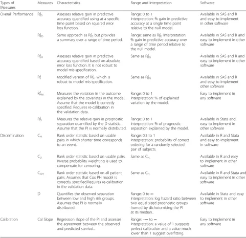
A brief summary of the performance measures is given in Table 1.
Results
Case study to illustrate the performance measures
A case study is now presented using the breast cancer data in order to describe how the performance measures may be evaluated in a validation setting. The dataset was split randomly into two parts with two thirds of the data used for model development and one third used for model validation. A Cox model was fitted to the devel-opment data using the same predictors as in Sauerbrei and Royston’s Model III [19] and the predicted prognos-tic index was calculated for all patients in the validation data using the estimated regression coefficients β̂. The values of all performance measures are shown in Table 2 with 95% confidence intervals estimated using the boot-strap techniques based on 200 bootboot-strap samples. For those measures that require specification of a time-point
τ, 3 years was deemed to be clinically appropriate. This was also the median follow-up time.
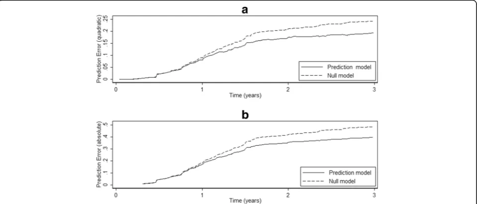
The estimated prediction errors used to estimate R2BSand
R2IBSare shown in Fig. 1a. The errors for the prediction and
null models are similar for the first 12 months after which the superiority of the prediction model is evident. The cor-responding prediction errors used to estimate R2SHappear
similar in shape although the magnitude of the errors are larger due to the use of an absolute loss function (Fig. 1b). The prediction errors used to estimate R2Sare almost
indis-tinguishable from those used to estimate R2SH(results not
shown). R2IBS, R2SH and R2S were estimated after averaging
the prediction errors over the first 3 years. As expected R2SH
and R2S are very similar, and both are slightly larger than
R2IBS. R2BSwas estimated using just the prediction errors at
3 years in Fig. 1a. Its value is larger than that of R2IBSas the
separation between the prediction errors is close to its max-imum at this time-point.
To estimate R2PMin the valids first re-calibrated for
rea-sons explained earlier. That is, the Cox model h tðjη̂Þ ¼h0
t
ð Þexpðα η̂Þwas fitted to the validation data, where η̂ is the predicted prognostic index calculated using the regression coefficients estimated in the development data. R2PM was then estimated using α̂
2
Varð Þη̂ rather than Varð Þη̂ . No such re-calibration is required to estimate R2D since, unlike R2PM, it uses the observed
survival outcomes in the validation data. The values of R2PM and R2D are very similar and noticeably larger
than the measures based on predictive accuracy (Table 2). We note that a naïve calculation (without re-calibration) of R2PM would have produced a much
larger value of 0.292, which would have provided an over-optimistic quantification of the model’s predictive performance.
The concordance measures CHand CUwere estimated
using all usable pairs in which shorter time corresponds to an event, and CGH was estimated after re-calibrating
the prediction model to the validation data as described above. The values of these 3 measures are all reasonably similar and would lead to similar conclusions in practice (Table 2). A naïve estimation of CGH (without
re-calibration) would have produced a much larger value of 0.696. Restricting the estimation of CH and CU by
censoring survival times in the validation data at 3 years produces slightly higher values for both measures, suggesting that the risk model has slightly better discrimination when considering survival over just the first 3 years. The D statistic suggests that the prediction model provides a reasonably high amount of prognostic separation (Table 2). Specifically, if one were to form two risk groups of equal size in the validation data, then the corresponding hazard ratio would be exp(0.998) = 2.71. The calibration slope estimate of 0.76 (equal to theα̂ esti-mated during the re-calibration process above) suggests that the prediction model has been slightly over-fitted. We note that, in practice, one can detect and adjust for model over-fitting during model development.
The selected measures all provide useful information. R2IBS, R2SH,and R2S, provide a summary measure
quantify-ing the improvement in predictive accuracy offered by the prediction model over the null model. The R2BS
measure is more appropriate if one is interested in predictive accuracy at a specific time-point, which is sometimes the case in practice. The prediction error curves provide additional insight into the performance of the prediction model at different time-points. R2PM
and R2D, which both quantify explained variation,
produced very similar values though calculation of R2PM
required a re-calibration of the prediction model. The concordance measures CH, CU and CGH produced
similar estimates, though calculation of CGH required
the prediction model to be re-calibrated. Additionally, if required, the calculation of CH and CUcan be restricted
Evaluation of the performance measures using simulation
Following the case study, a simulation study was per-formed to investigate how robust the measures are with respect to both censoring and the characteristics of the validation data. The simulation design is now described.
Simulation scenarios
The simulation study is based on the breast cancer and HCM datasets described earlier. For both datasets, de-velopment and validation datasets were generated by simulating new outcomes based on a true model and combining these with the original predictor values. Models were fitted in the development data and the
performance measures estimated in the validation data. Measures which require a choice of time-pointτ(including CH and CU) used 3 years for the breast cancer data and
5 years for the HCM data. These values were chosen as they are close to the respective median follow-up times in the original datasets and are conventional choices for sur-vival data. In practice, the choice of time-point would be clinically motivated and based on the underlying research question.
The performance measures were investigated over a range of scenarios to mimic real situations. For all simu-lations, validation data were constructed to have one of three different risk profiles (denoted low, medium, and Table 1Summary of the performance measures
Types of Measures
Measures Characteristics Range and Interpretation Software
Overall Performance R2BS Assesses relative gain in predictive
accuracy quantified using at a specific time point based on squared error loss function.
Range: 0 to 1
Interpretation: % gain in predictive accuracy at a single time point relative to the null model.
Available in SAS and R and easy to implement in other software
R2
IBS Same approach as R2BSbut provides
a summary over a range of time period.
Range: same as R2
BSInterpretation:
% gain in predictive accuracy over a range of time period relative to the null model.
Available in SAS and R and easy to implement in other software
R2SH Assesses relative gain in predictive
accuracy quantified based on absolute error loss function. It is not robust to model mis-specification.
Same as R2IBS Available in SAS and R and
easy to implement in other software
R2
S Modified version of R2SHwhich is
robust to model mis-specification.
Same as R2
IBS Available in SAS and R
and easy to implement other software R2
PM Measures the variation in the outcome
explained by the covariates in the model. Assume that the model is correctly specified. Requires re-calibration in the validation data.
Range: 0 to 1
Interpretation: % of explained variation by the model.
Easy to implement in any software
R2
D Measures the relative gain in prognostic
separation quantified by the D statistic. Assume that the PI is normally distributed.
Range: 0 to 1
Interpretation: % of prognostic separation explained by the model.
Available in Stata and easy to implement in other software Discrimination CH Rank order statistic based on usable
pairs in which shorter time corresponds to an event.
Range: 0.5 to 1
Interpretation: probability of correct ordering for a randomly selected pair of subjects.
Available in R and Stata and easy to implement in software
CU Rank order statistic based on usable pairs.
Inverse probability weighting is used to compensate for censoring.
Same as CH. Available in R and easy
to implement in other software
CGH Rank order statistic based on all patient
pairs. Assumes that Cox PH model is correctly specified.Requires re-calibration in the validation data.
Same as CH. Available in R and Stata and
easy to implement in other software
D Quantifies the observed separation between low and high risk groups. Assumes that PI is normally distributed.
Range: 0 to∞
Interpretation: log hazard ratio between two equal sized prognostic groups fromed by dichotomising the PI at its median..
Available in Stata and easy to implement in other software
Calibration Cal Slope Regression slope of the PI and assesses the agreement between the observed and predicted survival..
Range:−∞to∞
Interpretation: a value of 1 suggests perfect calibration and a value much lower than 1 suggest overfitting.
high). The use of different risk profiles reflect the fact that, in practice, the characteristics of the patients in the development and validation data may differ [36]. In par-ticular, the event rate for patients in the validation data may be higher or lower than that for patients in the de-velopment data due to differences in case-mix.
Four levels of random censoring were considered for the validation datasets (0, 20, 50, and 80%) which combined with the risk profiles, results in a total of 12 validation scenarios for each clinical dataset. The devel-opment datasets were generated with no censoring. 5,000 pairs of development and validation datasets were generated for each scenario.
Generating new survival and censoring times
Survival times were generated using the Weibull distri-bution as below
ts¼ −
logð Þu expð Þη
1
γ
where η and γ are the observed regression prognostic indices and shape parameter respectively (both used here as the proxy of the true values) anduis a uniformly distributed random variable on (0, 1). For the breast can-cer data, the prognostic indices and shape parameter were obtained by fitting a Weibull proportional hazards model using the same predictors as in Sauerbrei and Royston’s Model III [19]. For the HCM data, the prog-nostic indices were based on the regression coefficients estimated by O’Mahony et al. [20] and just the shape parameter was estimated using a Weibull model with the prognostic index specified as an offset.
To introduce random censoring, additional Weibull dis-tributed censoring times were simulated using tc= (−log(u)/
λ)1/γ where different choices of the scalar λ were used to give different proportions of censoring. A subject was con-sidered to be censored if their censoring time was shorter than their survival time.
Generating validation data with different risk profiles
The three different risk profiles were created in the validation data, by first splitting the patients into tertile risk groups based on their true prognostic index η. It is assumed that the first tertile group consists of low-risk patients, the second medium risk, and the third high-Table 2Values of the performance measures estimated in the
breast cancer validation data
Measure Value (95% CI)
R2
IBS(3) 0.107 (0.036 to 0.178)
R2
SH(3) 0.130 (0.089 to 0.171)
R2
S(3) 0.128 (0.090 to 0.167)
R2
BS(3) 0.141 (0.033 to 0.250)
R2
PM 0.194 (0.094 to 0.294)
R2
D 0.192 (0.093 to 0.291)
CH 0.674 (0.622 to 0.726)
CU 0.666 (0.610 to 0.722)
CGH 0.659 (0.616 to 0.701)
CH(3) 0.685 (0.633 to 0.737)
CU(3) 0.676 (0.619 to 0.734)
D 0.998 (0.672 to 1.323)
Cal. Slope 0.764 (0.531 to 0.996)
Fig. 1Prediction errors over time for the breast cancer risk model for:a) prediction error (based on a quadratic loss function) for calculating R2 IBS and R2BS;b) prediction error (based on an absolute loss function) for calculating R2
risk patients. The three risk profiles for the validation data were created in the following way:
a) low risk profile: 80% of the patients were sampled (without replacement) from the low-risk group, 50% from the medium-risk group, and 20% from the high-risk group;
b) medium risk profile: 50% of the patients were sampled from the low-risk group, 50% from the medium-risk group, and 50% from the high-risk group;
c) high risk profile: 20% of the patients were sampled from the low-risk group, 50% from the medium-risk group, and 80% from the high-risk group.
This sampling procedure was performed before gener-ating each validation dataset and resulted in validation datasets that were half the size of the original datasets. In contrast, no sampling of patients was performed when generating the development datasets; all patients were used.
The prognostic indices were approximately normally distributed for all risk profiles and for both datasets. There was slight skewness, particularly in the low and medium risk profile datasets. For example, the (average) skewness in the HCM datasets was 0.8 (low risk profile), 0.4 (medium) and 0.1 (high). There was a similar trend in the breast cancer datasets, although the values were lower. The variance was largest for the medium profile datasets which was to be expected considering the sam-pling scheme. This suggests that the medium profile datasets contained more prognostic information than the low and high profile datasets. Finally, there was more prognostic information in the breast cancer data, as evidenced by the wider range of the corresponding prognostic indices.
Simulation results
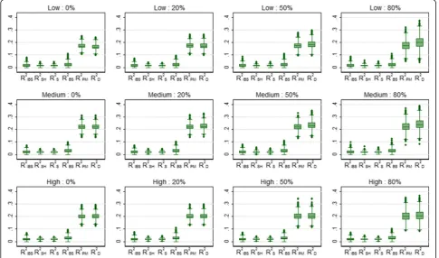
Table 3 shows the mean values of the overall performance measures over 5000 simulations for the breast cancer data, for the four levels of censoring and three risk profiles. The three summary measures based on predictive accuracy (R2IBS, R2SHand R2S) produced very similar values and were
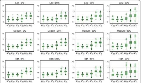
all unaffected by censoring. The values of these measures were highest for the medium risk profile simulations, where the patient characteristics were essentially the same in the development and validation samples, and lowest for the low risk profile simulations. Variability increased with increasing censoring, as expected, and was highest for R2IBS. This can clearly be seen in Fig. 2 which shows the
distribution of the values of the performance measures over the 5000 simulations (a few negative values were deleted to aid clarity). R2BS, evaluated at 3 years, was also
unaffected by censoring and achieved higher values in the
medium risk profile simulations. R2BSalso produced some
negative values (4%) when censoring was 80%. The two measures based on explained variation (R2PM and R2D)
produced similar values that were twice as large as the values obtained for R2IBS, R2SHand R2S. R2PMwas unaffected
by censoring but R2D increased slightly as censoring
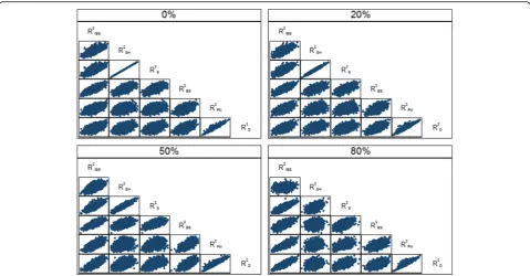
increased. The relationships between the various overall performance measures are shown in Fig. 3 for the medium risk profile scenario. In particular, there was excellent agreement between the R2SH and R2S measures which
weakened as censoring increased (ρ= 0.54 for 80% censoring). Also, there was good agreement between R2PM
and R2Dwhich seemed little affected by censoring (ρ= 0.95).
Very similar relationships were seen for the low and high risk scenarios (results not shown).
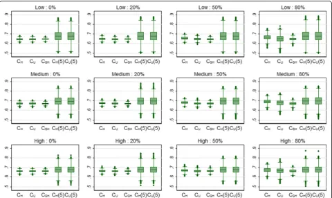
Table 4 shows the mean values of the discrimination and calibration measures for the breast cancer data. The Harrell and Uno c-indices were estimated twice, first using all usable patient pairs (CHand CU) and second by
restricting the calculations by censoring times greater than 3 years (CH(3) and CU(3)). For 0% censoring, the
CH and CGHmean values were very similar, and the CH
and CUestimates were identical by definition. CHtended
to increase as censoring increased, whereas CU and
particularly CGH were little affected. CGH was the least
variable of these three estimates. The variability in CH
and CU was similar except for 80% censoring where the
variability in CU was far larger (Fig. 4). The increased
variability was probably due to large values of the weights caused by the high degree of censoring. The mean value of CH(3) (and CU(3)) was slightly larger than
that for CH which suggests that the models were better
able to discriminate within the first 3 years compared to across the whole follow-up period. Both CH(3) and
CU(3) were relatively stable with respect to censoring,
and the variability of both measures was similar. The calibration slope and particular the D statistic showed a slight tendency to increase with censoring. The relation-ships between the discrimination measures are shown in Fig. 5 for the medium risk profile scenario. In particu-larly, there was reasonable agreement between the concordance measures and D. The strong relationship between CHand CH(3) for 80% censoring is explained by
the fact that there were few observed failure times above 3 years with this level of censoring. Very similar relation-ships were seen for the low and high risk breast cancer scenarios (results not shown).
negative R2IBS and R2BS values (11 and 9% respectively).
R2D was affected by censoring in the low and medium
risk profile simulations which may be explained by skewness in the prognostic index [6]. For example, the prognostic index was most skewed in the low risk profile HCM simulations, which is where greatest effect of censoring was observed. The relationships between the overall performance measures were similar, and often slightly stronger, than those seen in the breast cancer simulations (results not shown).
The results for the discrimination and calibration mea-sures for the HCM data can be seen in Table 6 and Fig. 7. As with the overall performance measures, the discrim-ination values were all lower than the corresponding values for the breast cancer data. CH was again badly
affected by censoring. In addition, D, like R2D, was also
affected by censoring in the low and medium risk profile simulations. Also notable is the increased variability of the CH(5) and CU(5) measures compared to their
unre-stricted counterparts. This again is due to the relatively Table 3Mean (SD) of the overall performance measures for the breast cancer data over 5000 simulations
Profile Censoring R2IBS(3) R
2
SH(3) R
2
S(3) R
2
BS(3) R
2
PM R
2 D
Low 0% 0.099 (0.032) 0.100 (0.018) 0.101 (0.018) 0.128 (0.037) 0.232 (0.034) 0.225 (0.034)
Low 20% 0.098 (0.033) 0.100 (0.019) 0.101 (0.019) 0.128 (0.038) 0.232 (0.038) 0.228 (0.038)
Low 50% 0.099 (0.034) 0.101 (0.019) 0.101 (0.019) 0.129 (0.040) 0.234 (0.045) 0.238 (0.048)
Low 80% 0.098 (0.041) 0.100 (0.024) 0.099 (0.023) 0.127 (0.060) 0.235 (0.065) 0.255 (0.075)
Medium 0% 0.131 (0.032) 0.133 (0.018) 0.135 (0.018) 0.176 (0.039) 0.279 (0.035) 0.277 (0.036)
Medium 20% 0.133 (0.032) 0.135 (0.018) 0.135 (0.018) 0.177 (0.040) 0.280 (0.038) 0.280 (0.038)
Medium 50% 0.131 (0.034) 0.135 (0.019) 0.134 (0.019) 0.176 (0.045) 0.279 (0.046) 0.283 (0.047)
Medium 80% 0.130 (0.045) 0.133 (0.025) 0.131 (0.025) 0.176 (0.082) 0.281 (0.068) 0.292 (0.071)
High 0% 0.121 (0.028) 0.123 (0.015) 0.125 (0.015) 0.165 (0.035) 0.247 (0.035) 0.243 (0.034)
High 20% 0.121 (0.028) 0.124 (0.016) 0.124 (0.016) 0.165 (0.038) 0.247 (0.038) 0.242 (0.037)
High 50% 0.121 (0.031) 0.125 (0.016) 0.124 (0.017) 0.164 (0.046) 0.247 (0.047) 0.243 (0.046)
High 80% 0.120 (0.048) 0.121 (0.022) 0.120 (0.026) 0.168 (0.114) 0.250 (0.070) 0.252 (0.071)
low number of events that occurred before 5 years and the consequent low number of patient pairs used to estimate both measures. Again, the relationships between the discrimination measures were similar to those seen in the breast cancer simulations (results not shown). In particular, there was excellent agree-ment between CGHand D (ρ= 0.99).
Discussion
The aim of this research was to review some of the promising performance measures for evaluating predic-tion models for survival outcomes, modify them if necessary for use with external validation data, and
perform a simulation study based on two clinical datasets in order to make practical recommendations.
Measures based on predictive accuracy quantify the predictive ability of the prediction model, relative to a null model with no predictors, on a percentage scale and can be readily communicated to health researchers. The measures investigated in this study (R2IBS, R2BS, R2SH and
R2S) may be estimated for any survival prediction model
provided that both the prognostic index and baseline survival function are available, although R2SHalso implicitly
assumes that the model is correctly specified [12]. If the baseline survival function is not available, which is usually the case in practice [6], then one approach might be to Fig. 3Scatter plot showing the relationshipsbetweenthe overall performance measures for the breast cancer data with the medium risk profile over 5000 simulations
Table 4Mean (SD) of the discrimination and calibration measures for the breast cancer data over 5000 simulations
Profile Censoring CH CU(τmax) CGH CH(3) CU(3) D Cal. Slope
Fig. 4Box plots showing the distribution of the concordance measures for 3 risk profiles (low, medium and high) and 4 levels of censoring (0, 20, 50 and 80%) for the breast cancer data over 5000 simulations
estimate it using the validation data. This is a pragmatic choice as the baseline survival function is rarely presented in practice by model developers. An alternative, arguably better, approach would be to estimate the baseline survival function for the prediction model (with covariates), but not the null model, using the development data. This alternative approach was investigated in the case study and produced very similar results (not shown). A negli-gible difference in the baseline survival function is also reported in [6] when it was estimated using development
and validation data separately. Similarly, for predic-tions from a null model, which are required for these measures, we suggest using the Kaplan-Meier estimate from the validation data.
Again for these measures, a choice of time-point is also required since the summary measures (R2IBS, R2SH
and R2S) are estimated over a specified range and R2BS is
estimated at a specified time-point. In practice, the choice of time-point will be guided by the clinical research question and the length of follow-up. For Table 5Mean (SD) of the overall performance measures for the HCM data over 5000 simulations
Profile Censoring R2IBS(5) R
2
SH(5) R
2
S(5) R
2
BS(5) R
2
PM R
2 D
Low 0% 0.013 (0.015) 0.013 (0.006) 0.014 (0.006) 0.020 (0.019) 0.173 (0.021) 0.166 (0.021)
Low 20% 0.013 (0.014) 0.013 (0.006) 0.013 (0.006) 0.020 (0.019) 0.173 (0.022) 0.173 (0.023)
Low 50% 0.014 (0.015) 0.013 (0.006) 0.013 (0.006) 0.020 (0.019) 0.174 (0.026) 0.184 (0.029)
Low 80% 0.014 (0.015) 0.014 (0.007) 0.014 (0.006) 0.020 (0.020) 0.174 (0.037) 0.201 (0.047)
Medium 0% 0.018 (0.014) 0.018 (0.006) 0.019 (0.006) 0.027 (0.019) 0.221 (0.022) 0.221 (0.023)
Medium 20% 0.018 (0.014) 0.018 (0.006) 0.019 (0.006) 0.027 (0.018) 0.221 (0.023) 0.226 (0.024)
Medium 50% 0.018 (0.014) 0.018 (0.006) 0.019 (0.006) 0.027 (0.019) 0.221 (0.028) 0.233 (0.031)
Medium 80% 0.018 (0.015) 0.018 (0.008) 0.019 (0.007) 0.027 (0.019) 0.222 (0.038) 0.241 (0.042)
High 0% 0.018 (0.013) 0.018 (0.005) 0.018 (0.005) 0.026 (0.017) 0.199 (0.022) 0.200 (0.022)
High 20% 0.018 (0.013) 0.018 (0.005) 0.018 (0.005) 0.027 (0.017) 0.199 (0.023) 0.201 (0.023)
High 50% 0.018 (0.013) 0.018 (0.006) 0.018 (0.005) 0.026 (0.017) 0.200 (0.028) 0.203 (0.029)
High 80% 0.018 (0.013) 0.018 (0.007) 0.018 (0.006) 0.026 (0.017) 0.201 (0.040) 0.206 (0.041)
example, it is common for risk to be estimated at 5 years [4, 20]. The four predictive accuracy measures studied were not affected by censoring in the simulation study. In addition, the three summary measures (R2IBS, R2SHand
R2S) produced very similar values on average. However,
the variability of R2IBSwas much greater than R2SHand R2S
which suggests that use of the latter two measures might be preferred in practice if a summary measure is required. Hielscher et al. compared two of these mea-sures, R2IBSand R2SH, and had similar findings [12].
The measures based on explained variation (R2PM and
R2D) may be estimated for any proportional hazards
model provided that the prognostic index is available, although we suggest that the prediction model is re-calibrated to the validation data before calculation of R2PM to ensure that the survival times in the validation
data are used in its calculation. Both measures provided very similar values in our simulations. R2PM was robust
to censoring, but R2Dtended to increase with censoring if
the prognostic index was skewed. Table 6Mean (SD) of the discrimination and calibration measures for the HCM data over 5000 simulations
Profile Censoring CH CU(τmax) CGH CH(5) Cu(5) D Cal. Slope
Low 0% 0.645 (0.011) 0.645 (0.011) 0.645 (0.009) 0.675 (0.061) 0.675 (0.061) 0.911 (0.070) 0.983 (0.082) Low 20% 0.649 (0.012) 0.645 (0.011) 0.645 (0.009) 0.676 (0.061) 0.676 (0.061) 0.934 (0.075) 0.986 (0.086) Low 50% 0.656 (0.016) 0.645 (0.014) 0.645 (0.011) 0.676 (0.062) 0.676 (0.062) 0.971 (0.095) 0.989 (0.098) Low 80% 0.666 (0.026) 0.649 (0.039) 0.645 (0.016) 0.676 (0.063) 0.676 (0.063) 1.025 (0.151) 0.988 (0.136) Medium 0% 0.670 (0.010) 0.670 (0.010) 0.670 (0.009) 0.694 (0.049) 0.694 (0.049) 1.090 (0.072) 0.985 (0.075) Medium 20% 0.674 (0.012) 0.670 (0.011) 0.670 (0.009) 0.695 (0.048) 0.695 (0.048) 1.105 (0.077) 0.986 (0.079) Medium 50% 0.680 (0.015) 0.670 (0.013) 0.670 (0.011) 0.694 (0.049) 0.694 (0.049) 1.127 (0.097) 0.985 (0.091) Medium 80% 0.688 (0.022) 0.675 (0.033) 0.670 (0.015) 0.695 (0.050) 0.695 (0.050) 1.153 (0.134) 0.989 (0.115) High 0% 0.661 (0.011) 0.661 (0.011) 0.661 (0.009) 0.676 (0.043) 0.676 (0.043) 1.022 (0.070) 0.982 (0.079) High 20% 0.663 (0.011) 0.661 (0.011) 0.661 (0.010) 0.677 (0.043) 0.677 (0.043) 1.025 (0.075) 0.983 (0.083) High 50% 0.667 (0.015) 0.661 (0.013) 0.661 (0.011) 0.676 (0.043) 0.676 (0.043) 1.032 (0.092) 0.984 (0.097) High 80% 0.672 (0.023) 0.664 (0.034) 0.661 (0.016) 0.676 (0.044) 0.676 (0.044) 1.042 (0.133) 0.987 (0.132)
Concordance measures are routinely used in practice since the concept of correctly ranking patient pairs can be readily communicated to health researchers [5]. CH
and CU can be estimated for any survival prediction
model that is able to rank patients. In addition, the calculation of CU may also be restricted to a specified
range of time, which may be useful to match with clinical aims or to compare concordance across different datasets. The calculation of CH may also be restricted
though it is not clear how often this is done in practice [37]. CGH has a similar interpretation to the other
concordance measures but requires that the model is correctly specified. As with R2PM, we suggest that the
prediction model is re-calibrated to the validation data before calculation of CGH to ensure that the survival
times in the validation data are used. Harrell’s CH, in its
unrestricted form, is probably the most used concord-ance measure in practice [5]. However, it was affected by censoring, which is a finding noted by others [16]. Specifically, CHtended to increase for moderate to high
levels of censoring, which is not an uncommon scenario with medical data, and is therefore likely to give an over-optimistic view of a prediction model’s discriminatory ability. Therefore, it cannot be recommended in such scenarios. In contrast, both CUand CGHwere reasonably
stable in the presence of censoring. CGH was the less
variable of the two measures as a consequence of it being model-based [16]. The restricted versions of CH
and CUwere little affected by censoring but care needs
to be taken when selecting the time-point to ensure that the time period contains a reasonable number of events.
The remaining discrimination measure D has an appealing interpretation as it can be communicated as a (log) relative risk between low and high risk groups of patients. It requires that the proportional hazards assumption holds and that the prognostic index is normally distributed. As with R2D it may be
affected by censoring if the prognostic index is skewed [27]. The sole calibration measure under investigation, the calibration slope, was robust to censoring. It assumes that the proportional hazards assumption holds although more general approaches are described by van Houwelingen [33, 38].
Conclusions
Harrell’s CH is routinely reported to assess discrimination
when survival prediction models are validated [5]. However, based on our simulation results, we recommend that CUis
used instead to quantify concordance when there are moderate levels of censoring. Alternatively, CGH could be
considered, especially if censoring is very high, but we suggest that the prediction model is re-calibrated first. The restricted version of CHmay also be used provided that the
time-point is chosen carefully. We also recommend that D
is routinely reported to assess discrimination since it has an appealing interpretation, although the distribution of the prognostic index would need to be checked for normality. ‘Overall performance’ measures are perhaps under used in practice. Our recommendation would be to use any of the predictive accuracy measures and provide the corresponding predictive accuracy curves. In particular, R2SH and R2S have relatively low
variability. The calibration slope is a useful measure of calibration and recommended to report routinely. In addition, one could investigate calibration graphically, for example by comparing observed and predicted survival curves for groups of patients [6]. Finally, we also recom-mend to investigate the characteristics of the validation data such as the level of censoring and the distribution of the prognostic index derived in the validation setting before choosing the performance measures.
Abbreviations
FP:Fractional Polynomial; HCM: Hypertrophic Cardiomyopathy
Acknowledgements
The authors would like to thank Drs Constantinos O’Mahony and Perry Elliott for allowing their data to be used data for simulation purposes. Also the authors would like to thank two reviewers and editor for their suggestions which strengthen the paper a lot.
Funding
This work was undertaken at University College London/University College London Hospitals who received a proportion of funding from the United Kingdom Department of Health’s National Institute for Health Research Biomedical Research Centres funding scheme. In addition, Babak Choodari-Oskooei is funded by Medical Research Council, grant number 532193-171339.
Availability of data and materials
The breast cancer dataset is available in a public domain at http:// biostat.mc.vanderbilt.edu/DataSets under the authority of the department of biostatistics, Vanderbilt University, USA. and sudden cardiac death data is available on request from Professor Perry Elliott at email: [email protected].
Authors’contributions
GA and MSR carried out the statistical analysis and simulation studies, and drafted the manuscript. BCO and RO input into the manuscript. All authors read and approved the final manuscript.
Competing interests
The authors declare that they have no competing interests.
Consent to publication
Not applicable.
Ethics approval and consent to participate
As the breast cancer dataset is freely available in public domain at http:// biostat.mc.vanderbilt.edu/DataSets and is permitted to use in research publication, the ethics approval consent statement from the ethical review committees at German Breast Cancer Study Group has been available to the authority who made the data available for public use. Again, Professor Perry Elliott (with email [email protected]) has given his consent to use HCM dataset for research paper and approval from ethical review committees at Heart Hospital, UK.
Publisher’s Note
Author details
1Institute of Statistical Research and Training, University of Dhaka, Dhaka,
Bangladesh.2Department of Statistical Science, University College London,
London, UK.3Institute of Clinical Trials & Methodology, University College London, London, UK.
Received: 2 January 2017 Accepted: 3 April 2017
References
1. Omar RZ, Ambler G, Royston P, et al. Cardiac surgery risk modeling for mortality: a review of current practice and suggestions for improvement. Ann Thorac Surg. 2004;77:2232–7.
2. Moons KGM, Royston P, Vergouwe Y, et al. Prognosis and prognostic research: what, why and how? Br Med J. 2009;338:1317–20.
3. Ambler G, Omar RZ, Royston P, et al. Generic, simple risk stratification model for heart valve surgery. Circulation. 2005;112:224–31.
4. Hippisley-Cox J, Coupland C, Vinogradova Y, et al. Predicting cardiovascular risk in England and Wales: prospective derivation and validation of QRISK2. Br Med J. 2008;336:1475–82.
5. Collins GS, de Groot JA, Dutton S, et al. External validation of multivariable prediction models: a systematic review of methodological conduct and reporting. BMC Med Res Methodol. 2014;14:40.
6. Royston P, Altman DG. External validation of a Cox prognostic model: principles and methods. BMC Med Res Methodol. 2013;13:33. 7. Harrell FE. Regression Modeling Strategies. Springer. 2001. 8. Steyerberg EW. Clinical Prediction Models: A Practical Approach to
Development, Validation and Updating. New York: Springer; 2009. 9. Steyerberg EW, Vickers AJ, Cook NR, et al. Assessing the performance of
prediction models: a framework for traditional and novel measures. Epidemiology. 2009;21(1):128–38.
10. Royston P, Altman DG. Visualizing and assessing discrimination in the logistic regression model. Stat Med. 2010;29(24):2508–20.
11. Schemper M, Stare J. Explained variation in survival analysis. Stat Med. 1996; 15:1999–2012.
12. Hielscher T, Zucknick M, Werft W, Benner A. On the prognostic value of survival models with application to gene expression signatures. Stat Med. 2009;29(7–8):818–29.
13. Choodari-Oskooei B, Royston P, Parmar MKB. A simulation study of predictive ability measures in a survival model I: Explained variation measures. Stat Med. 2012;31(23):2627–43.
14. Choodari-Oskooei B, Royston P, Parmar MKB. A simulation study of predictive ability measures in a survival model II: explained randomness and predictive accuracy. Stat Med. 2012;31(13):2644–59.
15. Pencina MJ, D’Agostino RB, Song L. Quantifying discrimination of Framingham risk functions with different survival C statistics. Stat Med. 2012; 31(15):1543–53.
16. Schmid M, Potapov S. A comparison of estimators to evaluate the
discriminatory power of time-to-event models. Stat Med. 2012;31(23):2588–609. 17. Austin PC, Pencinca MJ and Steyerberg EW. Predictive accuracy of novel risk
factors and markers: A simulation study of the sensitivity of different performance measures for the Cox proportional hazards regression model. Stat Methods Med Res.2015, in press.
18. Schmoor C, Olschewski M, Schumacher M. Randomized and non-randomized patients in clinical trials: experiences with comprehensive cohort studies. Stat Med. 1996;15:263–71.
19. Sauerbrei W, Royston P. Building multivariable prognostic and diagnostic models: transformation of the predictors by using fractional polynomials. J R Stat Soc A Stat Soc. 1999;162:71–94.
20. O’Mahony C, Jichi F, Pavlou M, et al. A novel clinical risk prediction model for sudden cardiac death in hypertrophic cardiomyopathy (HCM-RISK). Eur Heart J. 2014;35:2010–20.
21. Cox DR. Regression models and life tables. J R Stat Soc Ser B. 1972;34:187–220. 22. Stata Corporation. Stata Statistical Software, Release 13. College station: Tex:
Stata Corporation; 2013.
23. Graf E, Schmoor C, Sauerbrei W, Schumacher M. Assessment and comparison of prognostic classification schemes for survival data. Stat Med. 1999;18:2529–45.
24. Schemper M, Henderson R. Predictive accuracy and explained variation in Cox regression. Biometrics. 2000;56:249–55.
25. Schmid M, Hielscher T, Augustin T, Gefeller O. A robust alternative to the Schemper-Henderson estimator of prediction error. Biometrics. 2011; 67(2):524–35.
26. Kent J, O’Quigley J. Measures of dependence for censored survival data. Biometrika. 1988;75(3):525–34.
27. Royston P, Sauerbrei W. A new measure in prognostic separation in survival data. Stat Med. 2004;23:723–48.
28. Nagelkerke NJD. A Note on a General Definition of the Coefficient of Determination. Biometrika. 1991;78:691–2.
29. Harrell FE, Lee KL, Mark DB. Multivariable prognostic models: issues in developing models, evaluating assumptions and adequacy, and measuring and reducing error. Stat Med. 1996;15(4):361–7.
30. Uno H, Cai T, Pencina MJ, D'Agostino BD, Wei LJ. On the C-statistics for evaluating overall adequecy of risk prediction procedures with censored survival data. Stat Med. 2011;30:1105–17.
31. Gönen M, Heller G. Concordance probability and discriminatory power in proportional hazards regression. Biometrika 2005;92(4):1799–09. 32. Kaziol JA. The concordance index C and the Mann-Whitney parameter
Pr(X > Y) with randomly censored data. Biom J. 2009;51(3):467–74. 33. van Houwelingen HC. Validation, calibration, revision and combination of
prognostic survival models. Stat Med. 2000;19:3401–15.
34. Cox DR. Two Further Applications of a Model for Binary Regression. Biometrika. 1958;45:562–5.
35. Miller ME, Hui SL, Tierney WM. Validation techniques for logistic regression models. Stat Med. 1991;10(8):1213–26.
36. Justice AC, Covinsky KE, Berlin JA. Assessing the Generalizability of Prognostic Information. Ann Intern Med. 1999;130:515–24.
37. Pencina MJ, D’Agostino RB. Overall C as a measure of discrimination in survival analysis: model specific population value and confidence interval estimation. Stat Med. 2004;23:2109–23.
38. Choodari-Oskooei B, Royston P, Parmar MKB. The extension of total gain (TG) statistic in survival models: properties and applications. BMC Med Res Methodol. 2015;15:50.
• We accept pre-submission inquiries
• Our selector tool helps you to find the most relevant journal
• We provide round the clock customer support
• Convenient online submission
• Thorough peer review
• Inclusion in PubMed and all major indexing services
• Maximum visibility for your research
Submit your manuscript at www.biomedcentral.com/submit