Extensions to Study Electrochemical Interfaces - A Contribution to the Theory of Ions

Extensions to Study Electrochemical Interfaces, A

Contribution to the Theory of Ions

ALFREDHUBER

(COMMUNICATED BYIVANGUTMAN)

Constantly A-8062 Kumberg, Prottesweg 2a, Austria

ABSTRACT. In the present study an alternative model allows the extension of the Debye-Hückel Theory (DHT) considering time dependence explicitly. From the Electro-Quasistatic approach (EQS) done in earlier studies time dependent potentials are suitable to describe several phenomena especially conducting media as well as the behaviour of charged particles in arbitrary solutions acting as electrolytes.

This leads to a new formulation of the meaning of the nonlinear Poisson-Boltzmann Equation (PBE). If a concentration and/or flux gradient of particles is considered the original structure of the mPBE will be modified leading to a new nonlinear partial differential equation (nPDE) of the third order. It is shown how one can derive classes of solutions for the potential function analytically by application of an algebraic method. The benefit of the mathematical tools used here is the fact that closed-form solutions can be calculated without any numerical approximations.

Keywords: Nonlinear partial differential equations, DebyeHückel theory, PoissonBoltzmann equation.

1.

P

RELIMINARIES

We summarize some known ideas and give a short overview whereby the remarks are far from being complete. We restrict us as short as possible however some important notes should indicate a historical point of view. There is a good historical reason to deal the subject. When the developments of interefacial electrochemistry along modern lines became restricted by the overthermodynamics attidude of its adherents in the pre-1950 days, much attention was diverted to what had seemed previously to some extent the accompanying side issues, i.e. the physical chemistry of the bulk solution adjoining the

_{Corresponding author (Email:[email protected])}

double layer. This had concentrated upon an interest in the deviations in the behaviour of solutions from laws derived on the assumption that interaction between particles in them was negligible. It is known that the properties of electrolyte solutions can significantly deviate from the laws used to derive the chemical potential of solutions. In non-electrolyte solutions the intermolecular forces are mostly comprised of weak Van der Waals interactions, which have a _r7_{dependence (in principle), and for practical purposes this}

can be considered as ideal. In ionic solutions, however, there are significant electrostatic interactions between solute-solvent as well as solute-solute molecules. These electrostatic forces are governed by Coulomb's law which has a _r2_{dependence. Consequently, the}

1. 1. ELECTROMAGNETICS FROM AQUASISTATICPERSPECTIVE

General theory can be found in [27], [28], and [29]. Here only the essentials are cited. The quasistatic limit of the Maxwell Equations (MEs) is a kind of c limit (the fields propagate at once) obtained by neglecting time retardation. EQS has important applications modelling transient phenomena in approximating theories for materials with low conductivity (or low-frequency approximation). The crucial step is the fact that the time-dependent electric field may derived from a scalar potential which is, in our case the solution of a certain nPDE of the third-order [30]. Transient electrodynamical problems are not easy to solve in general, e.g. by occurring solutions depending on roots we have to take into account branch points. In media with a finite conductivity a static field is not possible and the pertinent relaxations time is given by 0/ [28], where  is the relative

permittivity and  the conductivity.

For metals (e.g. copper) the relaxation time is in the range of ₁₀18_{s. Otherwise,}

new developments on the material sector produces materials with a relative dielectric constant in the range 24 and a conductivity of about ₁₀9_{S/m. Then the decay rate is}

approximately _103_{s and this is long compared to other time constants of the system}

(e.g. an electromagnetic field passes through a panel). This is exactly the field where EQS can be applied [28], [29] and only pure capacitive effects are of interest. In further studies considering both capacitive and inductive effects the Darwin model will be used. Note that statics is just a particular case of the general MEs but quasistatics is an approximation.

2.

D

ERIVATION OF THE

M

ODEL

E

QUATION

It is stressed that the basic assumption of the DHT is the connection between the electrostatic Poisson equation and the Boltzmann distribution. However, this needs some assumptions: (i) the forces are shortranged, (ii) only Coulomb forces are undertaken (no dispersion forces),(iii)the involved particles are assumed to be point-like and unpolarized, (iv)the dielectric constant of the solution is assumed to be the same as the solvent and (v) electrolytes are dissociated completely. To derive the new model equation one starts from the MEs [11]:

t B E

rot

   

 

, rotH j D_t E E_t je

  

  

          

 ₀ ,

0

 B

Note:The fields E,B,D and Hare assumed time-dependent explicitly. Also the impressed current density and the charge density are functions of both arguments. However in this study the material constants are assumed as scalar quantities, that means (t)and(t).

It is assumed that there is both a weak current density due to the electric field and an impressed current densityj_e. The EQS assumption now means that the sources act slowly so that the fields change slowly and the conductivity  is rather small. Therefore the magnetic fields (the solenoidal part of the electric field) are negligibly small. From the EQS assumption one sets 0

 

t

B _{or 0}

    

t E t

D  _{. For that reason the electric field is derived}

from a scalar potential, so that one has the conclusion that the rotation of the magnetic part

vanishes: E gradu

t B E

rot   

  

 

 

0 . Taking the divergence of the second equation of

(2.1) one derives at an equation containing the unknown potential function u u(x,t)

depending upon their time derivative:

te e

j div u t u

     

 

    

 ₀ r . (2.2)

Then the concentration of particles due to diffusion will be considered. In general diffusion requires a gradient of the concentration of the particles. Under ‘balanced’ conditions the situation may be regarded as tantamount to equilibrium because there is no net flux or transport of ions. Hence, the Boltzmann law can be used. The argument is, that, since the field varies along the x-direction, the concentration of the ions at any distance x is given by

  

 

kT u e i z c

i

c ₀exp 0 , (2.3)

where u(x,t)is the potential energy of an ion in the applied field and c0is the concentration

in a region where the potential energy is zero (as x). Differentiating one obtains

u kTi

c dx du kT kT

u e i z c

dxi

dc _{ }

  

 

 ₀exp 0 1 r . (2.4)

Otherwise, from Fick’s law one has a contribution to the current density of the form

u kT

c FD z dx dc FD z

j i

i i i

D   



, (2.5)

      _          u kT c FD z t t

divjD i



0 _{. (2.6)}

For the second contribution it is obvious from the DHT that



         N i i i i

e ze N z e_kT u 1

0 0

0 exp , uu0 uL. (2.7)

0

u is the potential at any surfaces and u_L is the potential in the electrolyte far away from a reference ion (for further discussion we set u_L 0, hence u₀ u); z_i is the charge number, e₀ the elementary charge, k the Boltzmann constant, T is the temperature and

0

i

N is the particle number in the bulk, F the Faraday’s constant and D means the diffusion coefficient. So one has both contributions of the r.h.s. of eq.(2.2) and the new model equation reads as

0 exp 1 0 0 0

0 _

                  _{ }           



 N i i i i

iFD_kTc u _t ze N z_kTe u

z t u t

u  . (2.8)

Note: Precisely for the charge density a mean value is used in eq.(2.7) and  is the

Laplacian. For further considerations one-valued ions are assumed so that zi z1.Both the

arguments of the potential function u(x,t)will be suppressed, that means simply .

) , (x t u

u   The potential function u(x,t)urepresents the ion’s potential surrounded by the ‘ion cloud’. In further meaning this function describes the time-dependent potential of an arbitrary metal electrode (due to the restrictions underlying by the EQS not all metals can be considered) dipping in a liquid electrolyte. Note that a standard concentration of

l mol

c0,01 / , resp. c_ifor the concentration of the i-th ion at a standard temperature of K

T 293,15 is assumed (T 20oC).

For the following we take the conversion for the concentration: Let

i A

i N c

N01000 _{, where}

i

c is the molar concentration and considering the ion strength by 



i i i

z c

I 2

2

1 _{we introduce}

I T k N e z c T k N e A

i i i

A       



1000 2 2 1 1000 2 0 2 2 2 0

2 _{, (2.9)}

kT ze₀   , kT Dc 

2 _{. (2.9a)}

Finally one derives at the following nPDE of the third-order for the unknown time-depending potential function u u(x,t):

0 2 2 2 2 2 2 3               

 _u

e t u t x u x u t x

u _{. (2.10)}

At this stage let us impose formally boundary conditions so that _xlim_u0 uL and

0

lim _ 

dx du

x holds; they are necessary conditions later for the function uu(x,t). We

seek for solutions for the nPDE, eq.(2.10) for which uF(x,t), _FC3_{(D), DR}2 _{is an}

open set and further we exclude D:



(u(x,t))D~:u0,u_x 0,u_t 0,...



and a positive time t 0. Suitable classes of solutions are uI, Ian interval so that I D and

2

:I R

u  . Since it is always not an easy task to solve nPDEs analytically we wish to solve the nPDE, eq.(2.10) analytically by use of an algebraic method. In the following note we summarize the basic facts of the hyperbolic tangent method [31], [32] which is used below (only the basic steps are proposed).

Note:Consider a given nPDE in its two independent variables x and t

0 , , ... , , , ,

, 2₂ 1_{1 }

                      n n n n x u x u t u x u x u t u x u u

P . (a)

Firstly the nPDE converts into a nonlinear ordinary differential equation (nODE) by using a frame of reference u(x,t) f(), xt and  is a constant to be determined. Thus one

has



f(),f ('),f' ('),....



0

Q . (b)

The next step is that the solution can be expressed in terms of the following series representation by using an auxiliary variable () such that

) ( ) ( ) , ( 0     



 n i i i a f t x

u . (c)



1 ( )



)

('  ₁ 2  

  

 k

d

d _(d)

and k1 means a constant. The parameter n in eq.(c) is found by balancing the highest

derivative with the nonlinear terms in the reduced nODE eq.(b). Moreover, this parameter must be a positive integer since it represents the number of terms in the series (c). In the case of fractions one can take transformations as shown later. Substituting (c) and (d) into the relevant nODE will yield a system of nonlinear polynomial equations with respect to

0

a ,a1 , …. , k1 and .Solutions of the Riccati Equation can be expressed depending upon

the constant k1



 





 

) ₁tanh ₁

( k k

w , w() k₁coth



k₁



, for k₁0, (e)

 

 

 





) ₁tan _{1 1}cot ₁

( k k k k

w . for k₁0. (f)

Remark:The case k₁0 will be excluded here although a solution exists [31]. It represents

a useless solution for our purposes. To prevent confusions with the Boltzmann constant the character kis marked.

2. 1. THE APPLICATION OF THE HYPERBOLIC TANGENT METHOD – SOLUTION PROCEDURE

We convert the eq.(2.10) by u(x,t) f(), xt to derive the nODE of the third-order

0 ] exp[

2 2 2 2 2 2

3 3

             

 f

d f d d

f d d

f d d

f

d _{, f  f(), . (2.11)}

Note: The similarity transformation is called the traveling wave reduction describing any wave propagation and  means the velocity. However if we assume the EQS model

solutions of electromagnetic field problems can not represent traveling waves.

We seek for solutions for which vF(), where _FR3 _{and D R}2 _{is an open}

set and further we exclude D:



(f,)D~: f()0



. Suitable solutions are vI, I an interval so that I D and _{v:I R}2_{. Since the l.h.s of eq.(2.11) is a continuous function}

we ensure at least existence locally and due to the lemmas both from Peano and Picard-Lindelöf we assume uniqueness (also at least locally) in a given domain.





0 2 2                     f e d d d f d d f d d f d d

d _{. (2.12)}

Integrating once with C as an arbitrary constant of integration gives a second-order nODE

0 2 2 2 2             

 _e _C

d f d d f d d f

d f _{. (2.13)}

Note: During calculations it could have been shown that one can set the integration constant equal to zero without loss of generality. Here this constant will act as an arbitrary calculation quantity without any relation to the problem.

The transformation ( ) 1ln[ ()]

 

 w

f will remove the exponential function

yielding a further second-order nODE for the new dependent variable w():

0 2 2 2 2 2                       w d dw w d w d w d dw d w d

w , ww(). (2.14)

To apply the algorithm performed in the note above it is necessary to know the quantity n

in the series representation of eq.(c). It can be shown that two values exists: n₁ 1 and 2

2 

n . This is not possible since this quantity must be n+. Introducing further a new dependent variable p() by the transformations 1

1() p()

w and 2

2() p()

w will

give a second-order nODE for the function p():

0 3 2 2 2 2 2                       p d p d p d p d p d p d d p d

p . (2.15)

Note: Further analysis has shown that the inverse quadratic transformation only led to trivial solutions. We stress that p0is the singular point of this nODE.

The balancing procedure will result into two cases: (i) n₁ 1 and(ii) n₂ 2. Case (i) results into trivial solutions thus the quadratic form 2

2 1 0

)

( a a v a v

. 0 2 ... ... ... ... 0 2 2 3 0 2 1 1 0 2 1 2 2 0 2 1 2 1 1 1 0 2 2 2 1                a k a a k a a k a k a a a k (2.16)

From the seven solutions totally the only non-trivial solution yields

   ₂12 0 2k

a , a₁ 0,

    ₂12

2 2k

a , 1₂

 

 , k₁ 0, 0, 0, 0. (2.17)

Transforming back a compact written form for the potential function is given by







2 1 tanh



. ln 1 ) ( ) ,

(x t f 2 const

u   

   

 , _{xt xt}2_{, 0. (2.18)}

or explicitly in terms of time and space variables

. tanh 1 2 ln ) , ( 2 0 const c D t T k x e z T k t x u                    

 . (2.18a)

For further calculations the exponential form may be preferred; so we have

 





 





                                 

 ₂2 ₂

2 exp 1 4 exp 1 4 ln 1 . 1 2 ln 1 . ) ( const B A const

f , (2.18b)

with Ae  e  and B e  e .

Note: In order to realize real-valued solutions the constant k1must be k10and the root

terms become positive (during analysis we assumek11). Moreover eq.(2.18) is the only

appropriate solution for the chemical problem since the second solution of eq.(e) becomes singular. To ensure non-vanishing solutions the argument of the logarithm function must be greater than identity (that means that the relation2



1tanh2 



1holds).

From the laws of logarithms it follows that _const1_ln

 

_2 _{. This contribution will}

act as a shift for the(f,)curve. For imagination a concrete example is given: Consider the

values for KCl in water [33] and inserting the relevant quantities ones derived at

95 , 1 .

-0.5 0.5 1 1.5 2 2.5 3 x

-0.125 -0.1 -0.075

-0.05 -0.025 0.025

f

H

x

L

-3 -2 -1 1 2 3 x

-1.95 -1.9 -1.85 -1.8

f

H

x

L

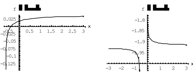
Figure 1.Comparison Between the Regular Solution Eq. 2.18.

Left containing the hyperbolic tangent function and the singular solution containing the hyperbolic cotangent,

Right. The regular solution covers the boundary condition so that the solution tends to a finite value. Taking a limit analysis one can prove lim_ f()0,035. This finite value can be interpreted as a finite potential value in any electrolytes. The first derivative exists (meant as the second boundary condition) and vanishes as  as to be required. The

positive branch of the singular solution may be considered as a potential starting on a conducting surface leading into a constant value in any liquids.

2. 2. A NUMERICALSTATEMENT

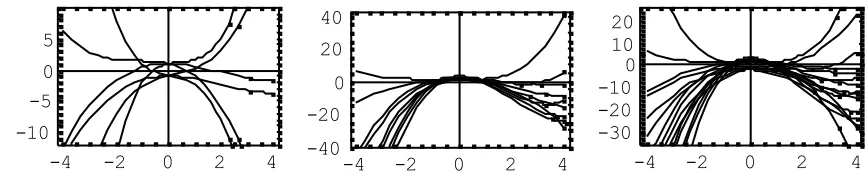
As mentioned above the highly nPDE eq.(2.11) and all nODEs derived from it, especially the nODE eq.(2.15) can only be solved under special circumstances, e.g. any similarity transformations. It is clear that by applying numerical standard procedures a closed-form solution is always obtained (considering suitable boundary and/or initial conditions). One of these standard procedures is the representation in ascending power series which is useful in numerical calculations. At the regular point 0 of the nODE eq.(2.15) one can assume a series representation up to order four in the form (here we set the constants ,  equal to identity and 2 since they do not influence the result necessarily):

 

4 3

2 0 3 1 0

2 1 1 2 0 2

0 2 1 1 2 0 1

0 1₄ 2 2 ₂₄1 2 6 12

)

( _  

  

  

   

     

  

  

  

 O

a a a

a a a a

a a a a

a

p (2.19)

with arbitrary chosen coefficients a0,a1 but a0 0.In figure 2 some integral curves are

-4 -2 0 2 4 -10

-50 5

-4 -2 0 2 4

-40 -20 0 20 40

-4 -2 0 2 4

-30 -20 -100

10 20

Figure 2. Some integral curves of the nonlinear nODE, eq.(2.15) generated by the series representation eq.(2.19).

Different values of the coefficients aiare used. Left the domain

) 1, 1 ( ) , ( ) 1, 1

(  a0 a1   , middle the domain (,13)(a0,a1)(11,)and right the domain )

1, 1 ( ) , ( ) 3 , 2

(  a₀ a₁   . Parabolic forms of the potential function and behaviour of the order

three is evident in the positive as well as negative directions.

3. A

NALYSIS

Let us summarize in short: Our main task was to solve the nPDE, eq.(2.10) in an analytical way dispensing any numerical approaches. This can be done by keeping in mind the special function methods. Although the eq.(2.10) is highly nonlinear, algebraic methods can therefore be applied successfully. A closed-form solution was then derived by the explicit formula for the time-dependent solution function eq.(2.18). By taking a limiting analysis it was shown that the potential function eq.(2.18) satisfies the required boundary conditions. Now we are interested in further quantities. The electric field can then derived from the potential (we further use the variable ) by application of the gradient operator (E) to give

   

   





 



 





   



 

  

 



 

 

4 exp 1 2 exp 1

1 2

exp 2

exp 2 tanh

2 sec )

( h

E , 0, (3.1)

where we have converted the hyperbolic functions into an exponential representation and

2

      

 

 





 

 



     



   

 sec 2sec 2 sec 2 tanh

8 1 )

( h2 h2 h , 0. (3.2)

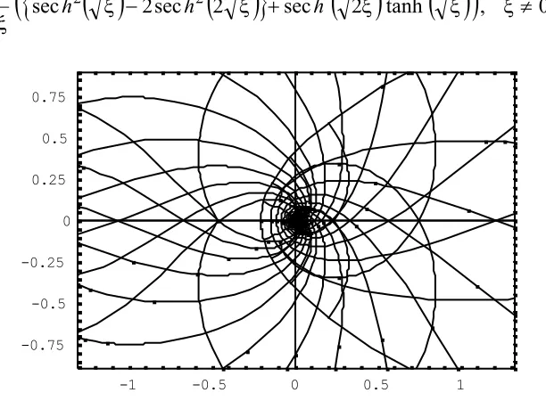
-1 -0.5 0 0.5 1

-0.75 -0.5 -0.25 0 0.25

0.5 0.75

Figure 3. The electrical field distribution derived from eq.(3.1). It can be shown that the field is of conservative character since by considering Cartesian coordinates, e.g.

) , , (_x _y _z 

 the relation rotE0 holds (it means that the field is irrotational or

equivalently, the existence of the potential is secured since the curl of the field vanishes).

To show that the field is really solenoidal one introduces Cartesian coordinates for the electric field, eq.(3.1) so that E (Ex,Ey,Ez)



. Then we have per definition with a unit

vector e_i:

z y

z y z z x

z x y y x

y x x z y x

z y x

z y x

E E e E E e E E e E E E

e e e E E

rot               

    

. (3.1.a)

Now it follows that (only the first component E_x is considered)

0 ... ...

tan 2 cosh tan

2

cosh _{   }

 

x x x

y y y

E

rot _{x y} , x0, y0. (3.1.b)

The charge density represents an analytical function except as 0 where the function is singular. From a limiting analysis it can be shown that the charge density vanishes as

 

 , that is lim()0 



 . Also it can be shown that for small values of the charge

density, that is 0, the charge density will take a finite value such that

   



That means by considering an arbitrary surface this surface will be charged by the given amount of charges of 7/12.

Let a be a specific distance (e.g. from the electrode surface to the centre of the hydrated ions in the OHL, the Outer HelmholtzLayer). The total charge qtot contained in

the OHL is obtained by integrating the charge density () from the electrode surface with the reference point taken at infinity. Therefore we have from eq.(3.2):

   





 



Exp a





Exp

 

a



a Exp a Exp d

q

a

tot 



() _{2 1} 2 _{2 1}2_ ₄1



, (3.3)

and qtot takes a function of the distance a.To avoid singularities one has to exclude special

values of the denominator, e.g. _a



0,_9_2/16,_2/4,_2/16



_{, and, for completeness}

some complex numbers _a



_log2



_(1)1/4



_{, log}2



_(1)3/4





_.

Let us study two limit cases: (i) for small distances, say, a0, the total charge tends to a constant factor: qtot 1/4 (this may be interpreted as the square of the first

spherical harmonics 2 00

Y );(ii)for large distances it is shown that q_tot 0 as a. This is also in agreement with the boundary conditions assumed earlier and matches our expectation exactly. In the following figures we show the charge density derived from the eq.(3.2) compared with the total charge density from the eq.(3.3).

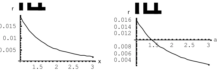
1.5 2 2.5 3 x 0.005

0.01 0.015

r

H

x

L

1.5 2 2.5 3 a

0.004 0.006 0.008 0.012 0.014

0.016r

H

a

L

Figure 4. Comparison between the charge density from eq.(3.2) as a function of the dependent variable  left and the total charge density as a function of the distance

acalculated from eq.(3.3).

3. 1. FURTHERPROPERTIES OF THEINVOLVEDQUANTITIES

one can calculate an alternating representation as 0 (but the series diverges). Thus a convergent series as 1 is given by



















_{0,202 1 0,120 1}2 _{0,064 1}3 _{0,032 1}4





₁



5

1 )

(         

  

 A O

f , (3.4)

where we have used the abbreviation

   

 

   const. ,1151

A and const. from above.

The convergence is relatively slow but in first order approximation a linear dependence is a good compromise. In the same manner for the electrical field it follows from, Eq. (3.1)















_{0,202 0,2405 1 0,1922 1}2 _{0,1330 1}3





₁



4

1 )

(        

 

 O

E . (3.5)

Since the function takes singular as 0the series is taken up from the point 1.

Note:One can asks if the potential function eq.(2.18) is a square-integrable function. That means one has to find a real, finite constant Mso that the relation



__ f() 2dM

holds. Taking into account the laws of logarithm one can transform eq.(2.18) into a sum of logarithmic parts. The integration shows that all these sums diverge and the latter relation is not satisfied (thus f()L2(Rn)). Consider appropriate domains, e.g.01, the existence

of the constant Mis given and a normalization is feasible. This may be important by

representing the potential function in terms of orthonormalizations and closure relations related with different basis sets.

4. S

UMMARY

Let us summarize in short: Due to our special model one is able to show that a special form of the PBE could solved exactly without any numerical calculations. However some restrictions (due to the EQS assumption) have been taken into account. For this special model, four important quantities could derive: (i) The potential of an electrode and/or the potential distribution of some charged particles, (ii) the electric field around an electrode and/or the field distribution inside a medium,(iii)the charge density,(iv)the charge density in the OHL.

R

EFERENCES

1. P. Debye, E. Hückel, DebyeHückel theory of electrolytes, Z. Phys. 24, 185206, 1923.

2. H. Falkenhagen, G. Kelbg, Klassische statistik unter Berücksichtigung des Raumbedarfs der teilchen,Ann. Phys.446, 6064, 1952.

3. M. Born, Über die Beweglichkeit der elektrolytischen Ionen,Z. Phys. 1/3, 221249, 1920.

4. L. Onsager, Electric moments of molecules in liquids, J. Am. Chem. Soc. 58, 14861493, 1936.

5. H. Falkenhagen, Elektrolyte,Verlag von Hirzel, Leipzig, 1932.

6. R. J. Hunter, Foundations of Colloid Science, Vol. 1, Clarendon Press, Oxford, 1987.

7. J. Bockris, A. Reddy, Modern Electrochemistry, Vol. 1: Ionics,Plenum Press, New York, 2001.

8. G. Gouy, Sur la constitution de la charge électrique à la surface d'un électrolyte, J. Phys.9, 457466, 1910.

9. C. Brett, A. Brett, Electrochemistry Principles, Methods and Applications, Oxford Univ. Press, 1993.

10. D. L. Chapman, LI. A contribution to the theory of electrocapillarity, Philos. Mag.

25, 475481, 1913.

11. J. D. Jackson, Classical Electrodynamics, 3rd ed., John Wiley & Sons, New York, 1998.

12. K. Huang, Statistical Mechanics, 2nd_{Ed.,John Wiley & Sons, New York, 1990.}

13. O. Stern, Theory of a doubleelectric layer with the consideration of the adsorption processes,Z. Electrochem. 30, 508516, 1924.

14. D. C. Grahame,The electrical double layer and the theory of electrocapillarity,

Chem. Rev.41, 441501, 1947.

15. N. Bjerrum, Der Aktivitätskoeffizient der lonen, Z. Anorg. Allgem. Chem. 109, 275292, 1920.

16. T. Gronwall, V. La Mer, K. Sandved, Über den Einfluss der sogenannten höheren Glieder in der Debye-Hückelschen Theorie der Lösungen starker Elektrolyte, Z. Physik, 29, 358393, 1928.

17. L. Onsager, Theories of concentrated electrolytes,Chem. Rev.13, 7389, 1933. 18. J. G. Kirkwood, Theory of solutions of molecules containing widely separated

charges with special application to zwitterions, J. Chem. Phys.2, 351361, 1934. 19. J. C. Ghosh, The abnormality of strong electrolytes. Part I. Electrical conductivity of

20. M. von Smoluchowski, Molekularkinetische Theorie der Opaleszenz von Gasen im kritischen Zustand, sowie einiger verwandter Erscheinungen, Ann. Physik 25, 205226, 1908.

21. H. C. Parker,The conductance of dilute aqueous solutions of hydrogen chloride, J. Amer. Chem. Soc.45, 20172033, 1923

22. P. Walden, H. Ulich, Weitere Zahlen in der von Walden kritisch bearbeiteten Übersicht in LandoltBörnsteinRothScheel, Z.Phys. Chem.106, 4992, 1923. 23. M. Planck, Über die Potentialdifferenz zwischen zwei verdünntenLösungen binärar

Elektrolyte,Ann. Physik. Chem.40, 561576, 1890.

24. R. M. Fuoss, F. Accascina, Electrolytic Conductance, Interscience Publishers Inc., New York, 1959.

25. G. Kortüm, J. Bockris, Textbook of Electrochemistry, Vol. 1, Elsevier, Amsterdam, 1951.

26. G. Kortüm, Lehrbuch der Elektrochemie, 5th ed.,Verlag Chemie, Weinheim, 1972. 27. J. Larsson, Electromagnetics from a quasistatic perspective, Am. J. Phys.75 (3),

230239, 2007.

28. J. A. Stratton, Electromagnetic Theory,McGrawHill, New York, 1941.

29. H. A. Haus, J. R. Melcher, Electromagnetic fields and energy, Prentice Hall Inc., New York, 1989.

30. A. Huber, A new time dependent approach for solving electrochemical interfaces part I: theoretical considerations using Lie group analysis, J. Math. Chem. 48, 856875, 2010.

31. A. Huber, Solitary solutions of some nonlinear evolution equations, Appl. Math. Comput.166(2), 464474, 2005.

32. W. Malfliet, Solitary wave solutions of nonlinear wave equations, Am. J. Phys. 60 (7), 650654, 1992.