Vol. 4, No. 3, Year 2012 Article ID IJIM-00167, 15 pages Research Article
Failure Mode and Effects Analysis Using Data
Envelopment Analysis
A. Hadi-Vencheha∗, S. Hejazib, A. Forghania, S. N. Hejazic
(a)Department of Mathematics, Khorasgan Branch, Islamic Azad University, Khorasgan, Isfahan, Iran.
(b)Department of Management, Dehaghan Branch, Islamic Azad University, Dehaghan, Isfahan, Iran.
(c)Tarbiat Moallem University of Sabzevar, Sabzevar, Iran.
——————————————————————————————————
Abstract
In this paper, we propose a bounded DEA based model to measure the overall risk of fail-ure modes. In the proposed model risk is measfail-ured within the range of an interval, whose performance is definitely superior to any one. The risks, obtained from bounded DEA models, turn out to be all intervals and are referred to as interval risk, which combine the best and the worst relative risk in a reasonable manner to give an overall assessment of performances for all failure modes. Assessor’s preference information on input and output weights is also incorporated into bounded DEA models reasonably and conveniently. A practical example is provided to compare the proposed model with those in the literature.
Keywords : Failure mode and effect analysis (FMEA); Data envelopment analysis (DEA); Risk priority number.
——————————————————————————————————
1
Introduction
Failure mode and effects analysis (FMEA) has proven to be a useful and powerful tool in assessing potential failures and preventing them from occurring. According to definition of Chrysler [7] failure mode and effect analysis can be described as a set of purposeful activities to identify and evaluate potential failures in productions, processes and their effects. Failure means unability to fulfill to desired process or necessity function that results in a low quality a bind of problem or service as perceived as a reason of dissatisfication by the customer. FMEA is a preventation methodology that have the capacity to with engineering and permanent method. This method is very significant in showing potential failures in production, process and provides effective management for
the proposed approach was demonstrated by studying a maritime collision risk due to technical failures. Sharma et al. [17] used a fuzzy rule-based inference method and the grey theory for prioritizing failure modes. Fuzzy linguistic terms are used to represent the risk degree for O, S, D and RPNs in the fuzzy rule base. Chin et al. [14] proposed an FMEA using the group-based evidential reasoning (ER) approach to capture FMEA team members’ diversity opinions and prioritize failure modes under different types of uncertainties such as incomplete assessment, ignorance and intervals. The risk priority model was developed using the group-based ER approach, which includes assessing risk factors using belief structures, synthesizing individual belief structures into group belief structures, aggregating the group belief structures into overall belief structures, converting the overall belief structures into expected risk scores, and ranking the expected risk scores using the minimax regret approach (MRA). Wang et al. [21] proposed a definition for the fuzzy RPNs using fuzzy weighted geometric means (FWGM). The fuzzy RPNs can be calculated by using α-level sets and a linear programming model and defuzzified by the centroid defuzzification method for the final ranking of the failure modes. In the method, different combinations of O, S and D can produce different fuzzy RPNs only when assigning different importance weights to O, S and D. In spite of the fact that much effort has been paid to the improvement of RPN, the improved methods either need to specify or determine the weights of risk factors in advance or take no account of them at all. It is argued that the specification or determination of risk factor weights is not easy because different decision makers (DMs) may have distinct judgments or preferences. Different failure modes have different consequences. The specification or determination of a fixed set of risk factor weights for all the failure modes might be inappropriate, particularly in the case with a large number of failure modes. In other words, it might be a better choice to use different sets of risk factor weights for different failure modes when there are a large number of failure modes to be prioritized. In this aspect, Garcia et al. [11] proposed a fuzzy data envelopment analysis (DEA) approach for FMEA, which does not require specifying or determining risk factor weights subjectively. Their approach, however, was computationally very complicated and also could not produce a full ranking for the failure modes to be prioritized. In this study we present an integrated model based on a new DEA model and Chin’s approach [6] to prioritize the risk factors. It is shown that the proposed model has better discriminating power than the traditional DEA efficiency and Chin’s model [6].
The rest of the paper is organized as follows. In the following section, we review DEA models for FMEA. In section 3, we illustrate our proposed method. A numerical examples is provided in section 4 to demonstrate the potential applications of the proposed FMEA and its advantages. Conclusions appear in section 5.
2
DEA models for FMEA
In this section we give a brief description of DEA and the geometric average method-ology. Suppose we have a set of n peer DMUs, {DMUj : j = 1,2, ..., n}, which produce
multiple outputs yrj (r = 1,2, ..., s), by utilizing multiple inputsxij (i= 1,2, ..., m). Let
respectively. The efficiency of the DMUo(o= 1,2, ..., n) is measured as follow:
θ=
s
∑
r=1
µryro
m
∑
i=1
υixio
, (2.1)
where µr is the output weight and υi is the input weight. The optimistic efficiency and
pessimistic efficiency of DMUo is measured by the following DEA models, respectively:
max θo = s
∑
r=1
µryro
m
∑
i=1
υixio
s.t. θj = s
∑
r=1
µryrj
m
∑
i=1
υixij
≤1 j= 1, ..., n
µr, υi≥ε r= 1, ..., s, i= 1, ..., m
(2.2)
min φo = s
∑
r=1
µryro
m
∑
i=1
υixio
s.t. φj = s
∑
r=1
µryrj
m
∑
i=1
υixij
≥1 j= 1, ..., n
µr, υi ≥ε r= 1, ..., s, i= 1, ..., m
(2.3)
It is a common knowledge that optimistic efficiency and pessimistic efficiency should form an interval when measured under the same constraints such as α ≤
n
∑
r=1
uryrj ≤ 1, (j =
1, . . . , n) with 0 < α < min{θj∗/φ∗j}, j = 1, . . . , n. The efficiency interval of DMUj
could accordingly be expressed as [αφ∗j, θj∗] if the value ofα is small enough. To avoid the difficulty in determining the value of α, Wang et al. [21] suggested a geometric average efficiency, determined by
ϕ∗j =√αφ∗jθ∗j j = 1, ..., n, (2.4)
where θ∗j and ϕ∗j are respectively the optimistic and pessimistic efficiencies of DMUj(j=
DMU, but also its pessimistic efficiency. It measures the overall efficiency of a DMU and considers both sides of a coin. The integration of two extreme efficiencies, optimistic and pessimistic, into a geometric average efficiency is undoubtedly more meaningful and more comprehensive than the use of either of the two efficiencies.
When efficiency intervals [αφ∗j, θ∗j], j = 1, . . . , n, are compared through their geometric midpoints √φ∗jθ∗j, the rankings among the n DMUs depend only upon their geometric average efficienciesϕ∗j =√φ∗jθj∗, j= 1, . . . , n, and have nothing to do with the value ofα. This good property enables the decision maker not to worry about how to determine the value ofα. He/She can therefore leave it alone and compare directly the geometric average efficiencies of the nDMUs to determine their overall performances and rankings [6]. Suppose there are n failure modes denoted by FMi(i= 1, . . . , n) to be prioritized, each
being evaluated against m risk factors denoted by RFj(j = 1, . . . , m). Let rij, (i =
1, . . . , n;j = 1, . . . , m) be the ratings of FMi on RFj and wj be the weight of risk factor
RFj, (j = 1, . . . , m). Since the RPN defined as the product of three risk factors O, S and
D has been largely criticized for its mathematical formula and equal treatment of the risk factors, we define in this paper the risks of failures with a different mathematical form, which can be either of the following:
Ri = m
∑
j=1
wjrij , i= 1, ..., n, (2.5)
Ri = m
∏
j=1
rijwj. i= 1, ..., n, (2.6)
Eq.(2.5) defines the risk of each failure mode as the weighted sum ofmrisk factors, whereas Eq.(2.6) as the weighted product ofmrisk factors. For convenience to distinguish between the two risks, we refer to the risk determined by Eq.(2.5) as additive risk and the risk by Eq.(2.6) as multiplicative risk, respectively. It is worthwhile to point out that the defini-tion for additive risks was first proposed by Braglia et al. [1], who defined the RPN as the weighted sum of O, S and D, whereas the definition for multiplicative risks was first proposed by Wang et al [21], who defined the RPN as the fuzzy weighted geometric mean of the three risk factors O, S, and D, which they referred to as fuzzy risk priority number (FRPN).
The traditional DEA often assigns too many zeros to input and output weights, leading to optimistic efficiency being unreasonably high and pessimistic efficiency being extraor-dinarily low. To avoid this from happening in FMEA, we consider imposing a constraint on the ratio of maximum weight to minimum weight. According to Saaty’s AHP [19] method, the maximum value, as a ratio of the comparative importance of a criterion over another, can assume to be 9. We therefore constrain the ratio of maximum weight to minimum weight within the range of one and nine. That is,
1≤ max(w1, ..., wm) min(w1, ..., wm) ≤
9 (2.7)
• The pairwise comparison matrices in the AHP are the most widely used approaches for estimating the relative importance weights of decision attributes or criteria, in which the maximum ratio scale between the importance of two attributes or criteria are usually not greater than 9.
• Risk factors O, S and D are all evaluated using the ratings between 1 and 10, where 1 represents no risk. Accordingly, their relative importance should also be evaluated using similar ratings. Due to the fact that no importance makes no sense, the ratings used for evaluating the relative importance of risk factors should therefore be defined as 1–9 rather than 1–10. As a result, the maximum ratio between the importance of two risk factors is less than or equal to 9.
The left-hand-side of Eq.(2.7) is trivial and holds always. Its right hand side is equivalent to the following:
max {
wj
wk
, j, k= 1, ..., m;j̸=k
}
(2.8)
which can be further rewritten as
wj−9wk≤0, j, k= 1, ..., m;j̸=k (2.9)
According to the DEA models introduced,we know that optimistic efficiency and pes-simistic efficiency of DMUo is measured by (2.10) and (2.11):
max θo = s
∑
r=1
uryr0
m
∑
i=1
vixi0
s.t. θj = s
∑
r=1
uryrj
m
∑
i=1
vixij
≤1, j = 1, ..., n,
ur, vi ≥ε, r = 1, ..., s;i= 1, ..., m (2.10)
min φo = s
∑
r=1
uryr0
m
∑
i=1
vixi0
s.t. φj = s
∑
r=1
uryrj
m
∑
i=1
vixij
≥1, j = 1, ..., n,
According to above models , FMEA models built for measuring the maximum and mini-mum risks of each failure mode, as shown below:
Rmaxo = max Ro
s.t.
{
Ri ≤1, i= 1, ..., n,
wj −9wk≤0, j, k= 1, ..., m;k̸=j
(2.12)
Rmino = min Ro
s.t.
{
Ri ≥1, i= 1, ..., n,
wj −9wk≤0, j, k= 1, ..., m;k̸=j
(2.13)
where Ro is the risk of the failure mode under evaluation. The overall risk of each failure
mode is defined by Eq.(2.4) as the geometric average of the maximum and minimum risks of the failure mode. That is,
¯
Ri=
√
Rmax
i .Rmini , i= 1, ..., n (2.14)
Therefor, n failure modes FMi (i= 1, . . . , n) can be easily prioritized by their geometric
average risks Ri (i = 1, . . . , n). The above models (2.12) and (2.13) are developed for
additive risks. For multiplicative risks defined by Eq.(2.6), the maximum and minimum risk models can be built in the same way, but the ratings and risks need to be transformed into logarithmic scales for linearity. The two models are constructed as follows:
ln Rmaxo = max ln Ro
s.t.
{
lnRi ≤1, i= 1, ..., n,
wj −9wk≤0, j, k= 1, ..., m;k̸=j
(2.15)
ln Rmino = min ln Ro
s.t.
{
lnRi ≥1, i= 1, ..., n,
wj −9wk≤0, j, k= 1, ..., m;k̸=j
(2.16)
Accordingly, the geometric average risk is defined as
¯
Ri=
√
exp(lnRmax
i ).exp(lnRmini ), i= 1, ..., n. (2.17)
where EXP(.) is the exponential function.
3
Proposed model
In order to apply DEA method in determiningα value for FMEA risk methods, first we should define ideal failure item and anti-ideal one. It is known that in FMEA, failure item has the first priority an high risk. In other word it has the highest degree for risk factors.
Definition 1. Anti-ideal failure item is a virtual item that has the lowest degree among risk factors.
factors.
Based on the above definitions, we denote the input and output values of ideal DMU (IDMU) byxmini (i= 1, ..., m) & ymaxr (i= 1, ..., s) and denote the input and output values of anti-ideal dMU (ADMU) by xmaxi (i = 1, ..., m), yrmin(i = 1, ..., s). These values are determined as follows:
xmini = min
j {xij} and x max
i = max
j {xij}, i= 1, ..., m (3.18)
yrmin= min
r {yrj} and y max
r = maxr {yrj}, r= 1, ..., s (3.19)
According to the concept of efficiency, the efficiency of ADMU is defined as follows:
θADM U =
s
∑
r=1
uryrmin
m
∑
i=1
vixmini
(3.20)
Letθ∗
ADM U be the optimistic efficiency of ADMU; then it can be obtained from the
follow-ing fractional programmfollow-ing model:
max θADM U =
s
∑
r=1
uryrmin
m
∑
i=1
vixmaxi
s.t. θj = s
∑
r=1
uryrj
m
∑
i=1
vixij
≤1, j= 1, ..., n,
ur, vi ≥ε, r= 1, ..., s;i= 1, ..., m, (3.21)
The fractional programming model (3.21) is converted to the following LP model, which can be solved readily.
max θADM U = s
∑
r=1
uryminr
s.t.
s
∑
r=1
uryrj − m
∑
i=1
vixij ≤0, j = 1, ..., n, m
∑
i=1
vixmaxi = 1
Similarly, efficiency of IDMU is defined as
φIDM U =
s
∑
r=1
uryrmax
m
∑
i=1
vixmini
(3.23)
Assuming that φ∗IDM U is the pessimistic efficiency of IDMU, it can be obtained from the following fractional programming model
min φIDM U = s
∑
r=1
urymaxr
m
∑
i=1
vixmini
s.t. φj = s
∑
r=1
uryrj
m
∑
i=1
vixij
≥1, j = 1, ..., n,
ur, vi≥ε, r= 1, ..., s;i= 1, ..., m, (3.24)
which can be solved using the following LP model:
min φIDM U =
s
∑
r=1
urymaxr
s.t.
s
∑
r=1
uryrj − m
∑
i=1
vixij ≥0, j = 1, ..., n, m
∑
i=1
vixmini = 1
ur, vi ≥ε, r = 1, ..., s;i= 1, ..., m, (3.25)
Based on the above discussion, we have θADM U∗ ≤ min
j=1,...,n
{
θj∗}and θIDM U∗ ≥ max
j=1,...,n
{
θ∗j}. Now we determine the parameter for all intervals [αφ∗o, θ∗o] (j= 1, . . . , n).
min
j=1,...,n
{
θ∗j
/
φ∗j
}
≥
min
j=1,...,n
{
θ∗j}
max
j=1,...,n
{
φ∗j} ≥
θADM U∗
φ∗IDM U (3.26)
If we setα=θADM U∗
/
In additive risk mode, Rmaxo is calculated for ideal and anti-ideal failure item by using model (2.12). So the following eqnarray is used to calculateα value:
α=RAF Mmax
/
RmaxIF M (3.27) After determining α value, model (2.13) is rewritten by adding a new constraint.
Rmaxo = max Ro
s.t.
Ri ≤1, i= 1, ..., n,
Ri ≥α, i= 1, ..., n
wj−9wk≤0, j, k= 1, ..., m;k̸=j
(3.28)
So the above model is used for determining values of Rmaxo failure modes. As it is seen in model (2.13), α value has no roles in this model. So model (3.28) is used for calculating maximum risk and model (2.13) is used for calculating minimum risk by considering α. According to the results, the following eqnarray is used to calculate interval risk
[
RLj, RUj ]=[αRminj , Rmaxj ] (3.29) But the question is how we rank interval numbers? Various methods have been presented for ranking interval numbers.Yue method [23] is used for ranking interval numbers in the present study. This method is on the basis of degree magnitude possibility of an interval number rather than another.
The advantage of Yue method against Wang method [21] in ranking interval numbers is that interval magnitude, lower bound and upper bound of comparative numbers have significant effect on the ranking of interval numbers.While in Wang method, two interval number with the same lower bound have the same ranking only if upper bound of these two numbers would not be the maximum upper bound of ranking numbers.
The above model is developed for additive risks. For multiplicative risks defined by Eq.(2.6), we should calculate values Romax for Anti-ideal Item and Ideal Item of failure modes in the same way. Thenα value is determined by using Eq.(3.27). Regarding to the estimated α, model (2.15) is rewritten to determine Rmaxo for each item as follows:
ln Rmaxo = max Ro
s.t.
lnRi ≤1, i= 1, ..., n,
lnRi ≥ln(α), i= 1, ..., n,
wj−9wk≤0, j, k= 1, ..., m;k̸=j
(3.30)
After determination of maximum and minimum values by model (2.16), interval risk is calculated according to eqnarray (3.29) and the suggested method is used to prioritize failure items.
4
An illustrative example
In this section we provide a numerical example we illustrate the potential application of the proposal fuzzy FMEA.This example is taken from Pillay and Wang [16].
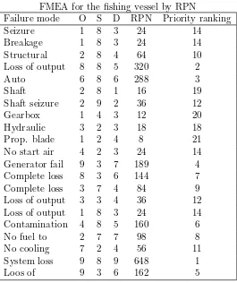
are structure, propulsion, electrical, and auxiliary systems. Each system is considered for different failure modes that could lead to an accident with undesired consequences. The effects of each failure mode on the system and vessel are studied along with the provisions that are in place or available to mitigate or reduce risk. For each of the failure modes, the system is investigated for any alarms or condition monitoring arrangements, which are in place. Table 1 show the 21 identified failure modes and their ratings on the three risk factors O, S, and D.
Table 1.
FMEA for the fishing vessel by RPN
Failure mode O S D RPN Priority ranking Seizure 1 8 3 24 14 Breakage 1 8 3 24 14 Structural 2 8 4 64 10 Loss of output 8 8 5 320 2 Auto 6 8 6 288 3 Shaft 2 8 1 16 19 Shaft seizure 2 9 2 36 12 Gearbox 1 4 3 12 20 Hydraulic 3 2 3 18 18 Prop. blade 1 2 4 8 21 No start air 4 2 3 24 14 Generator fail 9 3 7 189 4 Complete loss 8 3 6 144 7 Complete loss 3 7 4 84 9 Loss of output 3 3 4 36 12 Loss of output 1 8 3 24 14 Contamination 4 8 5 160 6 No fuel to 2 7 7 98 8 No cooling 7 2 4 56 11 System loss 9 8 9 648 1 Loos of 9 3 6 162 5
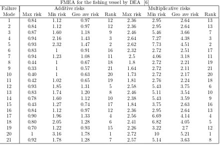
Table 2.
FMEA for the fishing vessel by DEA [6]
Failure Additive risks Multiplicative risks
Mode Max risk Min risk Geo ave risk Rank Max risk Min risk Geo ave risk Rank
1 0.84 1.12 0.97 12 2.36 2.95 2.64 13
2 0.84 1.12 0.97 12 2.36 2.95 2.64 13
3 0.87 1.60 1.18 9 2.46 5.46 3.66 7
4 0.94 2.16 1.43 3 2.64 7.27 4.38 3
5 0.93 2.32 1.47 2 2.62 7.73 4.51 2
6 0.83 1 0.91 16 2.32 2.72 2.51 17
7 0.94 1.23 1.08 11 2.5 4.06 3.18 11
8 0.44 1 0.67 18 1.8 2.72 2.21 19
9 0.33 1 0.57 21 1.64 2.72 2.11 21
10 0.40 1 0.63 20 1.73 2.72 2.17 20
11 0.42 1.02 0.65 19 1.81 2.76 2.24 18
12 0.93 1.85 1.31 5 2.58 5.43 3.75 6
13 0.83 1.74 1.20 8 2.46 5.11 3.54 10
14 0.78 1.60 1.12 10 2.38 5.43 3.59 9
15 0.43 1.27 0.74 17 1.84 3.75 2.63 16
16 0.84 1.12 0.97 12 2.36 2.95 2.64 13
17 0.90 1.96 1.33 4 2.56 6.69 4.14 4
18 0.80 2.05 1.28 6 2.41 6.82 4.05 5
19 0.70 1.22 0.93 15 2.26 3.22 2.7 12
20 1 3.16 1.78 1 2.72 10 5.21 1
21 0.92 1.78 1.28 7 2.57 5.14 3.63 8
4.1 Proposed model
In this case, first we should calculate values Rmaxo for Anti-ideal Item and Ideal Item. Anti-ideal Item and Ideal Item equals minimum and maximum failure modes. However risk factor raying of Anti-ideal Item and Ideal Item are as follow
Table 3
Ratings of Anti-ideal Item and Ideal Item factor risks
Failure modes O S D
Anti-ideal Item 1 2 1
ideal Item 9 9 9
By solving (3.22) and (3.25) for Anti-ideal Item and ideal Item, respectively,we get the following results for additive risk:
θ∗A−Ideal = 0.2222 and φ∗Ideal= 1.1, hence α= 0.12222.1 = 0.202. Regarding to the estimated
α, the following linear programming has been solved to determineRmaxo for each 21 items:
Rmaxo = maxRo
s.t.
Ri ≤1, i= 1, ..., n,
Ri ≥0.202, i= 1, ..., n,
wj−9wk≤0, j, k= 1, ..., m;k̸=j
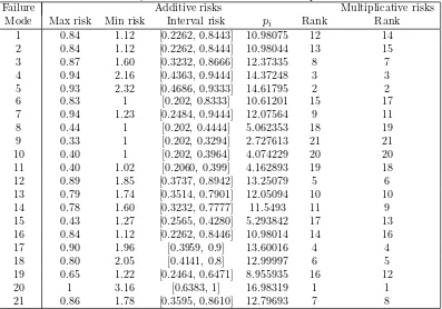
Table 4
Interval efficiency evaluation for additive and multiplicative risk.
Failure Additive risks Multiplicative risks
Mode Max risk Min risk Interval risk pi Rank Rank
1 0.84 1.12 [0.2262, 0.8443] 10.98075 12 14
2 0.84 1.12 [0.2262, 0.8444] 10.98044 13 15
3 0.87 1.60 [0.3232, 0.8666] 12.37335 8 7
4 0.94 2.16 [0.4363, 0.9444] 14.37248 3 3
5 0.93 2.32 [0.4686, 0.9333] 14.61795 2 2
6 0.83 1 [0.202, 0.8333] 10.61201 15 17
7 0.94 1.23 [0.2484, 0.9444] 12.07564 9 11
8 0.44 1 [0.202, 0.4444] 5.062353 18 19
9 0.33 1 [0.202, 0.3294] 2.727613 21 21
10 0.40 1 [0.202, 0.3964] 4.074229 20 20
11 0.40 1.02 [0.2060, 0.399] 4.162893 19 18
12 0.89 1.85 [0.3737, 0.8942] 13.25079 5 6
13 0.79 1.74 [0.3514, 0.7901] 12.05094 10 10
14 0.78 1.60 [0.3232, 0.7777] 11.5493 11 9
15 0.43 1.27 [0.2565, 0.4280] 5.293842 17 13
16 0.84 1.12 [0.2262, 0.8446] 10.98014 14 16
17 0.90 1.96 [0.3959, 0.9] 13.60016 4 4
18 0.80 2.05 [0.4141, 0.8] 12.99997 6 5
19 0.65 1.22 [0.2464, 0.6471] 8.955935 16 12
20 1 3.16 [0.6383, 1] 16.98319 1 1
21 0.86 1.78 [0.3595, 0.8610] 12.79693 7 8
In order to estimate multiplicative risk, we solved model (2.15) for Anti-ideal Item and Ideal Item that following results were obtained
θ∗A−Ideal = 1.3098 and φ∗Ideal = 2.8458 then α = 12..30988458 = 0.4630. Rankings prevented in the last column of Table 4 is calculated by determining α value and solving model (3.30) for 21 failure modes. It is clear from Table 3 that the Chin’s method could not provide a robust ranking. For example, FM1, FM2 and FM16 have the same additive risk rank. A
similar situation holds for multiplicative risk ranking. While our method overcomes this shortcoming. Out of 21 failure modes 12 modes have the same additive risk rank in both methods. Whereas, when we consider multiplicative risk 17 modes have the same rank in both methods.
5
Conclusion
In this paper we proposed a DEA based methodology for ranking failure mode risk in FMEA. In the proposed model each FM is considered as a DMU and its best and worse relative efficiency computed. Furthermore, theoretically the best and worst relative efficiency showed as an interval. For this purpose, a parameter called asαused to moderate the worst relative efficiency of DMUs. So it seems that the proposed model that uses α
Acknowledgment
The authors are grateful for the constructive comments and suggestions made by the two anonymous referees.
References
[1] M. Braglia, M. Frosolini, R. Montanari,Fuzzy criticality assessment model for failure modes and effects analysis, International Journal of Quality and Reliability Manage-ment 20 (2003) 503-524.
[2] M. Bevilacqua, M. Braglia, R. Gabbrielli, Monte Carlo simulation approach for a modified FMECA in a power plant, Quality and Reliability Engineering International 16 (2000) 313-324.
[3] M. Braglia, M. Frosolini, R. Montanari, Fuzzy TOPSIS approach for failure mode, effects and criticality analysis, Quality and Reliability Engineering International 19 (2003) 425-443.
[4] CL. Chang, CC. Wei, YH. Lee, Failure mode and effects analysis using fuzzy method and grey theory, Integrated Manufacturing Systems 12 (2001) 211-216.
[5] LH. Chen, WC. Ko, Fuzzy linear programming models for new product design using QFD with FMEA, Applied Mathematical Modelling 33 (2009) 633-647.
[6] KS. Chin, YM. Wang, GKK. Poon, JB. Yang, Failure mode and effects analysis by data envelopment analysis, Decision Support Systems 48 (2009) 246-256.
[7] Chrysler Corporation, Ford Motor Company, and General Motors Corporation, Po-tential Failure Mode and Effect analysis (FMEA) Reference Manual(1995).
[8] PDT. Connor, Practical Reliability Engineering, Heyden, London (2002).
[9] C. Ebeling, An Introduction to Reliability and Maintainability Engineering, Tata McGraw-Hill, New York (2001).
[10] F. Franceschini, M. Galetto,A new approach for evaluation of risk priorities of failure modes in FMEA, International Journal of Production Research 39 (2001) 2991-3002. [11] PAA. Garcia, R. Schirru, E. Frutuoso, PF. Melo, A fuzzy data envelopment analysis
approach for FMEA, Progress in Nuclear Energy 46(2005) 59-73.
[12] G. Ireson, W. Coombs, F. Clyde, YM. Richard, Handbook of Reliability Engineering and Management, 2nd ed., McGraw-Hill Professional, New York, (1995).
[13] JB.Bowles, CE. Pelaez,Fuzzy logic prioritization of failures in a system failure mode, effects and criticality analysis, Reliability Engineering and System Safety 50 (1995) 203-213.
[15] NASA, Failure Modes, Effects and Criticality Analysis (FMECA), Practice no. PDAP- 1307, (1999).
[16] A. Pillay, J. Wang, Modified failure mode and effects analysis using approximate reasoning, Reliability Engineering and System Safety 79 (2003) 69-85.
[17] RK. Sharma, D. Kumar, P. Kumar, Fuzzy modeling of system behavior for risk and reliability analysis, International Journal of Systems Science 39(2008) 563-581 [18] A. Segismundo, P. Augusto, C. Miguel, Failure mode and effects analysis (FMEA)
in the context of risk management in new product Development: A case study in an automotive company, International Journal of Quality and Reliability Management 25(2008) 899-912.
[19] TL. Saaty, The Analytic Hierarchy Process, McGraw-Hill, New York, (1980).
[20] RJ. Vokurka, SW. Leary-Kelly, A review of empirical research on manufacturing flexibility, Journal of Operations Management 18 (2000) 485-501.
[21] YM. Wang, KS. Chin, KKG. Poon, JB. Yang, Risk evaluation in failure mode and ef-fects analysis using fuzzy weighted geometric mean, Expert Systems with Applications 36(2009) 1195-1207.
[22] Z. Yang, S. Bonsall, J. Wang, Fuzzy rule-based Bayesian reasoning approach for pri-oritization of failures in FMEA, IEEE Transactions on Reliability 57 (2008) 517-528. [23] Z.Yue,An extended TOPSIS for determining weights of decision makers with interval