Vol. 10, No. 1, 2018 Article ID IJIM-00850, 10 pages Research Article
Computer Extended Series and HAM For the Solution of Non-Linear
Squeezing Flow of Casson Fluid Between Parallel Plates
Vishwanath B. Awati ∗†, Manjunath Jyoti ‡
Received Date: 2016-03-29 Revised Date: 2017-01-28 Accepted Date: 2017-10-22
————————————————————————————————–
Abstract
The paper presents analysis of two-dimensional non-Newtonian incompressible viscous flow between parallel plates. The governing problem of momentum equations are reduced to nonlinear ordinary differential equation (NODE) using similarity transformations. The resulting equation is solved using computer extended series solution (CESS) and homotopy analysis method (HAM). These methods have advantages over pure numerical methods for obtaining the derived quantities accurately for various values of parameters and results are valid in much larger parameter domain compared with numerical schemes.
Keywords: Squeezing flow; CESS; HAM; Casson fluid; Pade approximants.
—————————————————————————————————–
1
Introduction
T
hflow between two parallel plates moving nor-e two-dimensional incompressible viscous mal to the surface symmetrically about line of symmetry, gives rise to squeezing flow is very important because of its many widespread in-dustrial, biological and practical applications in many engineering fields. Squeezing flow between parallel infinite plates or discs is an interesting area of study in fluid mechanics; it has many applications including hydrodynamical machines, compression / injection modeling, flow inside sy-ringes and nasogastric tubes etc. Stephan [33] was the first researcher who initiated the pioneer-ing work on the squeezpioneer-ing flow under lubrication approach. Later Reynolds [31] and Architabald∗Corresponding author. await [email protected]. †Department of Mathematics, Rani Channamma Uni-versity, Belagavi-591156, India.
‡Department of Mathematics, Rani Channamma Uni-versity, Belagavi-591156, India.
[2] investigated the squeezing flow between ellip-tic plate and rectangular plate respectively.
The fluids involved are not simply Newtonian in most of realistic models, and a single model cannot capture the complex rheological proper-ties of non-Newtonian fluids. The different types of non-Newtonian fluids have been studied in different mathematical approaches; one of such model is Casson fluid model. McDonald [24] and Mrill et al. [26] showed that the most compati-ble formulation to simulate blood type fluid flows. Many researchers have contributed their investi-gation efforts towards the better understanding of squeezing flow in different geometries. Moham-mad et al. [25] and Ganesh et al. [15] discussed the problem for unsteady flow of MHD viscous fluid between two parallel plates through porous medium. Kirubhashankar et al. [18, 19] studied MHD flow of an electrically conducting viscous fluid between moving parallel permeable plates. Siddiqui et al. [32] examined the homotopy per-turbation solution for the MHD squeezing flow of
a viscous fluid between two plates. Mustafa et al. [27] analyzed heat and mass transfer charac-teristics in a fluid for the squeezing flow. Rashidi et al. [30] considered the problem of unsteady two dimensional squeezing flows between circu-lar plates. The MHD squeezing flow of viscous fluid has been studied by Umar Khan et al. [17] and the same problem was discussed by Naveed et al. [1] by invoking a magnetic field parameter to the problem. Ellahi et al. [12] discussed the non-Newtonian nanofluids with Reynolds model and Vogels model which are the illustrative mod-els of variable viscosity. In pure numerical meth-ods, a set of discrete points on a curve has been considered to obtain the solution of differential equations. Therefore it is often difficult and time consuming to get a complete path (curve) of re-sults. On the other hand, at each point within the domain of interest approximate analytical solu-tions are available. The analytical solusolu-tions pro-vide an effective initial guess to get approximate solution of nonlinear problem within few itera-tions. Many researchers are interested in obtain-ing semi-analytical and semi-numerical solutions of various nonlinear problems related to science and engineering fields. We reinvestigate the prob-lem of non-linear squeezing flow of a Casson fluid between parallel plates using semi-analytical / semi-numerical methods viz. computer extended series solution and found some useful and inter-esting results based on new type of series analysis. Van Dyke [34] and his associates have shown the probable applications of these methods in com-putational fluid dynamics. For simple models the semi-analytical and semi-numerical methods pro-posed here is to provide accurate results and have advantages over pure numerical schemes. The few manually calculated approximations in low Reynolds number perturbation solution of the boundary value problem, which enables us to pro-pose systematic series expansion to generate the universal polynomial coefficients by using recur-rence relation and Mathematica. The resulting series have limited radius of convergence by non-physical singularities, is extended to moderately high Reynolds numbers using an analytic contin-uation of series solution. The location and nature of singularity restricts the convergence of series is predicted by using Domb-Sykes plot [10]. The sign pattern of the coefficients decides the nature of singularity, then recast the series into
contin-ued fraction representation [7] and use Pade’ ap-proximants of various orders for summing it. Bu-jurke et al. [8, 9] studied the flow in a narrow channel of varying gap using computer extended series solution and his associates have used this technique successfully.
The alternative approach is to obtain analytic solution of the proposed problem using homotopy analysis method (HAM). The HAM was devel-oped by Liao [20] and further modified it in [21] to introduce a non-zero auxiliary parameter which is known as convergence-control parameter, which allows us to adjust the convergence region and rate of approximations of required solution. In general perturbation and asymptotic techniques are strongly dependent upon small / large pa-rameters which are often valid for solving weakly nonlinear boundary value problems. This method is free from small / large physical parameter, flex-ibility on choice of base function and initial guess. Also, HAM is used to solve highly nonlinear dif-ferential equations arising in engineering appli-cations, which has great flexibility and generality over all other analytical techniques. Recently, El-lahi [13, 14] discussed various aspects related to flow of non-Newtonian nanofluid and investigated the effects of MHD and temperature dependent viscosity by using HAM. Most recently, Awati et al. [4,5,6] used CESS and HAM for the solution of flow problems arising in fluid mechanics and shown potential applications of these methods.
The present paper is structured as follows. Sec-tion 1 describes the introduction of the problem. Section 2 Mathematical formulation of the pro-posed problem and relevant boundary conditions is given. Section 3 is devoted to the solution of the problem using CESS. Section 4 devoted to the solution by HAM. Section 5 presents the re-sults and discussion, and Section 6 is about the conclusion.
2
Mathematical Formulation
[11,28] as
τij = {
(µB+√p2yπ)2eij, π > πc,
(µB+√p2yπ)2eij, π < πc.
whereτij is the (i, j)-th component of stress ten-sor,π =eijeij andeij are the (i, j)-th component of deformation rate, π is the product component of deformation rate with itself,πcis critical value of product based on non-Newtonian model,µB is dynamic viscosity of non-Newtonian fluid andpy is the yield stress of fluid. The governing equa-tions of present flow problem become [24]
∂u ∂x+
∂v
∂y = 0, (2.1)
u∂u ∂x +v
∂u ∂y =
(
1 + 1 β
) (
∂2u
∂x2 +
∂2u
∂y2 )
, (2.2)
u∂v ∂x +v
∂v ∂y =
−1
ρ ∂p ∂y +ν
(
1 + 1 β
) (
∂2v ∂x2 +
∂2v ∂y2
)
(2.3)
whereuand vare the velocity components along xandydirections respectively,ν is the kinematic fluid viscosity, pbe the pressure, ρ is the density of fluid,β =µB
√ 2πc
py is the Casson fluid
parame-ter. The appropriate boundary conditions for the flow equations are
u(x, y) = 0, v(x, y) =v0 at y=h,
uy(x, y) = 0, v(x, y) = 0 at y= 0.
(2.4)
There is no slip condition at upper plate for the first two conditions and remaining two conditions follow from symmetry of the flow aty= 0. Elim-inating the pressure terms from Eqn. (2.2) and (2.3), after cross differentiation and invoking vor-ticity ω then simplify the above system of equa-tions, we get
u∂ω ∂x +v
∂ω ∂y =ν
(
1 + 1 β
) (
∂2ω ∂x2 +
∂2ω ∂y2
)
(2.5)
where ω = ∂x∂v −∂u∂y. Introducing the dimension-less similarity variable η= yh, where his the dis-tance between plates, then Eqns. (2.1) and (2.5) becomes ∂u ∂x + 1 h ∂v
∂η, (2.6)
u∂ω ∂x + v h ∂ω ∂η =ν (
1 + 1 β
) (
∂2ω ∂x2 +
1 h2
∂2ω ∂η2
)
(2.7) and the boundary conditions are
u(x, η) = 0, v(x, η) =v0 at η= 1,
uy(x, η) = 0, v(x, η) = 0 at η= 0.
(2.8)
Let ψbe a stream function is of the form
ψ(x, η) = [hU(0)−v0x]f(η) (2.9)
The velocity components u and v related to the physical stream function defined by
u(x, η) = ∂ψ ∂y =
1 h
∂ψ
∂η and v(x, η) =− ∂ψ ∂x, (2.10) where U(0) is the average entrance velocity at x= 0 and velocity components becomes
u(x, η) =
[
U(0)−v0 hx
]
f′(η)
and v(x, η) =v0f(η) (2.11)
Using Eqns. (2.11) the continuity equation sat-isfied automatically and the Eqns. (2.7) and (2.8) reduces to the nonlinear ordinary differen-tial equation
f′′′′+R
(
β 1 +β
) (
f′f′′−f f′′′), (2.12)
whereR= v0h
ν is Reynolds number. The relevant boundary conditions becomes
f(0) = 0, f′(1) = 0, f′′(0) = 0, f(1) = 0. (2.13)
3
Series Solution
We seek a solution of Eqn. (2.12) in powers ofR in the form
f(η) =
∞ ∑
n=0
Rnfn(η) (3.14)
Substituting Eqn. (3.14) into Eqn. (2.12) and equating like powers of R on both sides, we get
f0′′′′ = 0, (3.15)
fn′′′′+1=−( β 1 +β)[f
′
0f
′′ n+f
′ nf
′′
0 −f0f
′′′ n
−fnf ′′′
0 ]− n−1 ∑
L=1
( β 1 +β)[f
′ Lf
′′ m−fLf
′′′ m],
where m =n−L . The boundary conditions of the flow equations are
f0(0) = 0, f
′
0(1) = 0, f
′′
0(0) = 0, f0(1) = 0,
fn(0) = 0, f ′
n(1) = 0, f ′′
n(0) = 0, fn(1) = 0,
n= 1,2, ... (3.17)
The required solutions of the above equations up toO(R2) are
f0=
1
2(3η−η
3)
f1=−
1 280
(
β 1 +β
)
(2η−3η2+η7)
f2= (
β 1 +β
)
(− 703 1293600η+
73 107800η
3
+ 3 19600η
7− 1
3360η
9+ 73
92400η
11) (3.18)
The calculation of higher order terms manually of the series (3.16) is very difficult because the al-gebra becomes cumbersome. It is essential to get the higher order terms to approximate the func-tion properly and we cannot analyze the problem accurately by considering only these three terms of the series. The behavior of the solution (3.18) enables us to propose a systematic series expan-sion with universal polynomial coefficients, which is quite useful and more efficient in calculation of higher order approximations. The nature of solu-tions (3.18) suggest the general formfn(η) to be of the form
fn(η) = 2n ∑
k=1
A(n,2k−1)(1−η2)2η2k−1, n≥1.
(3.19) The above general form yields exactly the previ-ous calculated terms fi(i = 1,2), besides this it enables us to find for (i > 2) using the follow-ing recurrence relation and FORTRAN program-ming. Substituting Eqn.(3.19) into an Eqn.(3.14) and equating like powers of η on both sides and obtained a recurrence relation for unknowns
A(n,2k−1) in the form
A(n+1,4n−(2J+1)) = 2A(n+1,4n−(2J−1))
−A(n+1,4n−(2J−3))+
1
(4n−(2J−3))(4n−(2J −2))(4n−(2J−1))(4n−(2J))
× {[
4 ∑
i=1
A(4n−2i−2J+3)Pi(4n−i−J + 2)
+ n−1 ∑
L=1
[
2 ∑
r=−2
(
2L ∑
k1=2L−J+r
A(L,2k1−1)
·A(m,4n−2k1−(2J+(1−2r)))
·S(7−r)(k1, N2−k1−(J −r)))]]} (3.20)
where m = n − L and J varies from
−2,−1,0,1, ....(2n−1).
For obtaining other Aij’s, we use above recur-rence relation. The expression for radial velocity is given by
f′(η) = 3 2(1−η
2) + ∞ ∑
n=0
Rn
2n ∑
k=1
A(n,2k−1)
[(2k+ 3)η2k+2−2(2k+ 1)η2k+ (2k−1)η2k−2] (3.21)
The expression for pressure gradient of the series is given by
f′′′(0) =−3 +
∞ ∑
n=0
Rnan (3.22)
wherean=−6A(n,1)+ 6A(n,3). The analytic
con-tinuation of region and validity of series can be achieved by taking various Pade’ approximants. The coefficients of the series (3.21) and (3.22) representing the radial velocity f′(η) and pres-sure gradient f′′′(0) are decreasing in magnitude but having random sign pattern and results are further extrapolated using rational approxima-tion for determining the radius of convergence. Fig.1shows Domb-Sykes plot which confirms the radius of convergence after extrapolation of the series f′′′(0) to be R0= 26.32272 and 15.78283
for Casson fluid parameter β = 1 and 5 respec-tively. The direct sums of the series for radial and axial velocities are valid only up to the ra-dius of convergence. We use pade approximants for summing the series which gives a converging sum for sufficiently large Reynolds number R.
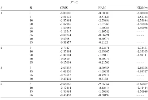
Table 1: Comparison of f′′′(0) results with CESS, HAM and numerical results for different Casson fluid parameterβ and Reynolds numberR.
f′′′(0)
β R CESS HAM NDSolve
1 0 -3.00000 -3.00000 -3.00000
5 -2.81135 -2.81135 -2.81135
10 -2.55884 -2.55884 -2.55884
20 -1.87965 -1.87966 -1.87966
25 -1.50986 -1.50986 -1.50986
30 -1.16547 -1.16542
-35 -0.86244 -0.86221
-40 -0.5908 -0.59074
-45 -0.31877 -0.3162
-2 5 -2.7347 -2.73471 -2.73471
10 -2.35364 -2.35365 -2.35365
20 -1.39104 -1.3911 -1.3911
30 -0.5819 -0.59074
-35 -0.15008 -0.21509
-3 5 -2.69358 -2.69358 -2.69358
15 -1.69336 -1.69337 -1.69337
25 -0.72517 -0.72414
-30 -0.30432 -0.3162
-5 5 -2.65056 -2.65057 -2.65057
10 -2.12414 -2.12414 -2.12414
15 -1.50984 -1.50986 -1.50986
25 -0.49493 -0.50192
-Figure 1: Domb-Sykes plot for the seriesf′′′(0) forβ= 1 and 5.
parameter on radial velocity for moderately large Reynolds number. An identical behavior is ob-served for almost all velocity profiles for Casson fluid parameter and Reynolds number.
4
Homotopy Analysis Method
We employ HAM [22, 23] for the solution of the flow problem (2.12) with boundary conditions
Figure 2: ¯hcurves for the seriesf′(0) for different values ofβ andR.
(2.13), it is straight forward to choose the initial approximation as
f0(η) =
3 2η−
1 2η
3 (4.23)
and auxiliary linear operator of the governing equation is defined as
Figure 3: ¯hcurve for the seriesf′′′(0) for different values ofβ andR.
Figure 4: Axial velocity curves for different val-ues ofRwhenβ = 2.
The above linear operator satisfies the following property
L[C1η3+C2η2+C3η+C4] = 0 (4.25)
where C1, C2, C3 and C4 are constants to be
de-termined later. Ifq∈[0,1] then the zeroth order deformation problem can be constructed as
(1−q)L[f(η, q)−f0(η)] =qhH(η)N[f(η, q)],
(4.26) subjected to the boundary conditions
f(0, q) = 0, f′(1, q) = 0,
f′′(0, q) = 0, f(1, q) = 1. (4.27)
where q ∈ [0,1] is an embedding parameter, ¯h and H are the non-zero auxiliary parameter and auxiliary function respectively. Further N is the nonlinear differential operator given by
N[f(η, q)] = ∂
4f(η, q)
∂η4 +R (
β 1 +β
)
[
∂f(η, q) ∂η
∂2f(η, q) ∂η2 +f
∂3f(η, q) ∂η3
]
(4.28)
Figure 5: Radial velocity curves for different val-ues ofRwhen β= 2.
Figure 6: Axial velocity curves for different val-ues ofβ whenR= 15.
For q = 0 and q = 1, Eqn. (4.26) have the solu-tion
f(η,0) =f0(η), f(η,1) =f(η) (4.29)
As q varies from 0 to 1, f(η, q) also varies from the initial guessf0(η) to the exact (final) solution
f(η). By Taylor’s theorem Eqn. (4.29) can be written as
f(η, q) =f0(η) + ∞ ∑
m=1
fm(η)qm (4.30)
where fm(η) = m1!∂
mf(η,q)
∂qm |q=0. The convergence
of above series strictly depends upon the conver-gence control parameter ¯h, and also assume that ¯
h is selected in such a way that the series is con-vergent at q= 1, then we have
f(η) =f0(η) + ∞ ∑
m=1
fm(η) (4.31)
Figure 7: Axial velocity curves for different val-ues ofβ whenR= 15.
Figure 8: Velocity profiles for moderately larger values ofRwhenβ= 1.
mth-order deformation problem becomes
L[fm(η)−χmfm−1(η)] =qHRm(η) (4.32)
and the homogeneous boundary conditions are
fm(0) = 0, f ′
m(1) = 0, f ′′
m(0) = 0,
fm′ (1) = 0, m≥1. (4.33)
where
Rm(η) =f ′′′′ m +R
(
β 1 +β
)
m∑−1
n=0
[fn′fm′′−n−1−fnf ′′′
m−n−1] (4.34)
and
χm= {
0, ifm≤1,
1, ifm >1. (4.35)
To solve the system of linear equations (4.32) with homogeneous boundary conditions (4.33) by
us-Figure 9: Velocity curves for moderately larger values ofRwhenβ = 2.
Figure 10: Velocity curves for moderately larger values ofRwhenβ = 5.
ing Mathematica software, we obtain solutions as
f1(η) = (
β¯hR (1 +β)
) (
1 140η−
3 280η
3+ 1
280η
7 )
f2(η) = (
β¯hR 140(1 +β) +
β¯h2R 140(1 +β)2
+ β
2¯h2R
140(1 +β)2 +
703β2¯h2R2
1293600(1 +β)2)η
+ (− 3β¯hR 280(1 +β) −
3β¯h2R 280(1 +β)2
− 3β2¯h2R
280(1 +β)2 +
73β2¯h2R2 107800(1 +β)2)η
3
+ ( β¯hR 280(1 +β) +
β¯h2R 280(1 +β)2
+ β
2¯h2R
280(1 +β)2 +
3β2¯h2R2 19600(1 +β)2)η
7
− β2¯h2R2
3360(1 +β)2η
9+ 3β2¯h2R2
92400(1 +β)2η 11
4.1 Convergence of HAM
The series (4.31) contains the auxiliary parame-ter ¯h. The convergence of series strictly depends on the parameter ¯h and is known as convergence control parameter, which influences the conver-gence rate and region of series. We draw ¯hcurves for velocity and pressure gradient at 10th order of approximations. To ensure that the permissible ranges of parameter ¯h, by drawing the line seg-ment of ¯h curves parallel to η-axis. From Fig. 2
and Fig. 3, it is observed that admissible ranges for ¯h are −2 ≤¯h ≤ 1.7 and −1.5 ≤ ¯h ≤ 1.7 for the series f′(0) and f′′′(0) for different values of Casson fluid parameter β and Reynolds number R. The computation shows that series converges in the whole region of 0≤η ≤1 when ¯h=−0.9.
5
Results and discussion
The nonlinear squeezing flow of an incompress-ible Casson fluid between two parallel plates is analyzed. The resulting nonlinear ordinary dif-ferential Eqn. (2.12) with boundary conditions (2.13) is solved by using CESS and HAM. By using both the methods the graphs of axial and radial velocity profiles have been drawn for dif-ferent Reynolds number R and Casson fluid pa-rameter β. The series expansion scheme with polynomial coefficients proposed here enables in obtaining recurrence relation. Using recurrence relation (3.20) and Mathematica, we generate large number (n = 30) of universal coefficients A(n,2k−1), k = 1,2, ...2n and n = 1,2, ...30. The velocity profiles are further improved by using Pade approximants for much larger values of R for different values of Casson parameter β which are shown in Figs. 8-10 and the profiles agree closely with HAM curves.
Fig. 4 shows that an increasing value ofR cor-responds to a decrease in the velocity along the y-direction for fixed Casson parameter β. Fig.
5 presents radial velocity profiles for increasing values of R corresponds to a decrease in velocity in the region η ≤ 0.5 and increase in the region 0.5≤η ≤1. Fig. 6 depicts the behavior of Cas-son fluid parameterβ, it is observed that the axial velocity decreases corresponds to increase in the values ofβ.
Fig. 7 shows that the radial velocity for in-crease in β corresponds to decrease in velocity in the region η ≤ 0.5 and increase in the region
0.5≤η≤1.
The coefficient of the series (3.22) representing pressure gradient f′′′(0) are decreasing in mag-nitude and having random sign patterns. Fig.1 shows Domb-Sykes plot which confirms the ra-dius of convergence after extrapolation of series f′′′(0) to beR0= 26.32272 and 15.78283 for
Cas-son fluid parameterβ = 1 andβ = 5 respectively. The direct sum of the series (3.22) is valid only up to the radius of convergence for different values of Casson fluid parameter β. We use the Pade’ approximant’s for summing up series which give a converging sum for sufficiently large Reynolds number. The pressure gradient results are com-pared between computer extended series solution and homotopy analysis method with numerical results, which agree very well with pure numeri-cal solutions for different Casson fluid parameter β and Reynolds numberR. The results are given in Table1.
6
Conclusion
In the present analysis, the non-linear squeezing flow of an incompressible Casson fluid between parallel plates is studied using CESS and HAM. The major observations are:
• The location and nature of singularity re-stricts the convergence of series is predicted quite accurately using Domb-Sykes plot.
• The region of validity of the series is ex-tended for much larger value of Reynolds number R.
• From the ¯h curves it is observed that 10th order approximations are enough to obtain the solutions of flow problem.
• Table 1 presents the validity of semi-numerical / semi-analytical methods results with numerical results.
References
[1] N. Ahmed, U. Khan, S. I. Khan, S. Bano, S. T. Mohyud-Din, Effects on magnetic field in squeezing flow of a casson fluid between par-allel plates,J. King Saud University- Science
[2] F. R. Archibald, Load capacity and time re-lations in squeeze films, Trans. ASME, J. Lub. Technol.(1956) 29-35.
[3] V. B. Awati, N. M. Bujurke, N. N. Katagi, Computer extended series solution for the ows in a Nonparallel channels, Advances in Applied Science Research 3 (2012) 2413-2423.
[4] V. B. Awati, M. Jyoti, N. N. Katagi, Com-puter extended series and Homotopy anal-ysis method for the solution of MHD flow of viscous fluid between two parallel porous plates,Gulf Journal of Mathematics4 (2016) 65-79.
[5] V. B. Awati, M. Jyoti, K. V. Prasad, Series analysis for the flow between two stretchable disks,Engg. Sci and Tech. Int. J. 20 (2017) 1211-1219.
[6] V. B. Awati, M. Jyoti, Homotopy analysis method for the solution of lubrication of a long porous slider,AMNS1 (2016) 507-516. [7] C. M. Bender, S. A. Orzag, Advanced Math-ematical Methods for Scientists and En-gineers, Third International Edition (Mc-Grawhill Book Company) (1987).
[8] N. M. Bujurke, V. B. Awati, N. N. Katagi, Computer extended series solution for flow in a narrow channel of varying gap, Applied Mathematics and Computation 186 (2007) 54-69.
[9] N. M. Bujurke, N. N. Katagi, V. B. Awati, Analysis of steady viscous ow in slender tubes,Z. angew. Math. Phys.56 (2005) 831-851.
[10] C. Domb, M. F. Sykes, On the susceptibil-ity of a ferromagnetic above the curic point,
Proc. Roy. Lond. Ser. A240 (1957) 214-228. [11] N. T. M. Eldabe, M. G. E. Salwa, Heat transfer of MHD non-Newtonian Casson fluid flow between two rotating cylinders,J. Phys. Soc. Japan64 (1995) 41.
[12] R. Ellahi, M. Raza, K. Vafai, Series solutions of non-Newtonian nanofluids with Reynolds model and Vogels model by means of the ho-motopy analysis method, Mathematical and Computer Modelling55 (2012) 1876-1891.
[13] R. Ellahi, The effects of MHD and tempera-ture dependent viscosity on the flow of non-Newtonian nanofluid in a pipe: Analytical solutions, Applied Mathematical Modelling
37 (2012) 1451-1467.
[14] R. Ellahi, A Study on the Convergence of Se-ries Solution of Non-Newtonian Third Grade Fluid with Variable Viscosity: By Means of Homotopy Analysis Method,Advances in Mathematical Physics(2012).
[15] S. Ganesh, S. Krishnambal, Unsteady stokes flow of viscous fluid between two parallel porous plates, Int. J. Information Science and Computing1 (2007) 63-66.
[16] S. Ganesh, C. K. Kirubhashankar, I. A. Mo-hamed, Non-Linear Squeezing Flow of Cas-son Fluid between Parallel Plates, Int. J. Math. Anal. 9 (2015) 217-223.
[17] U. Khan, N. Ahmed, S. I. Khan, S. Bano, S. T. Mohyud-din, Unsteady squeezing flow of a casson fluid between parallel plates,World J. Modell. Simul. 10 (2014) 308-319.
[18] C. K. Kirubhashankar, S. Ganesh, Unsteady MHD flow of a Casson fluid in a parallel plate channel with heat and mass transfer of chem-ical reaction, Paripex- Indian J. Research 3 (2014).
[19] C. K. Kirubhashankar, S. Ganesh, Unsteady MHD flow of a Casson fluid through parallel plate channel with heat source,Pensee Jour-nal76 (2014).
[20] S. J. Liao, The proposed homotopy analysis techniqe for the solution of nonlinear prob-lems, PhD Thesis, Shanghai Jiao Tong Uni-versity(1992).
[21] S. J. Liao, An explicit, totally analytic ap-proximation of Blasius viscous flow prob-lems, International Journal of Non-Linear Mechanics34 (1992) 759-778.
[22] S. J. Liao, Beyond perturbation: Introduc-tion to homotopy analysis method,Boca Ra-ton: Chapman Hall/CRC Press(2003). [23] S. J. Liao, Homotopy Analysis Method in
[24] D. A. McDonald, Blood flows in Arteries,
Second ed. Arnold. London(1974).
[25] A. Mohamed Ismail, S. Ganesh, C. K. Kirubhashankar, Unsteady Magnetohydro-dynamic flow between two parallel plates through a porous medium, Int. Jl. On Design and Manufacturing Technologies 7 (2013) 1-6.
[26] E. Mrill, A. M. Benis, E. R. Gilliland, T. K. Sherwood, E. W. Salzman, Pressure flow relations of human blood hollow fibers at low flow rates, J. Appl. Physiol. 20 (1965) 954-967.
[27] M. Mustafa, T. Hayat, S. Obaidat, On heat and mass transfer in the unsteady squeezing flow between parallel plates, Meccanica 47 (2012) 1581-1589.
[28] M. Nakamura, T. Sawada, Numerical study on the flow of a non-Newtonian fluid through an axisymmetric stenosis,ASME J. Biomech. Eng.110 (1988) 137.
[29] W. H. Press, B. P. Flannery, S. A. Teukolsky and W. T. Vetterling, Numerical Recipes,
Cambridge University Press(1986).
[30] M. M. Rashidi, H. Shahmohamadi, S. Di-narvand, Analytic approximate solution for unsteady two dimensional and axisymmetric squeezing flow between parallel plates, Math-ematical Probems in Engineering (2008) 1-13.
[31] O. Reynolds, On the theory of lubrication,
Trans. Royal Soc.(1886) 177-157.
[32] A. Siddiqui, S. M, Irum, A. R. Ansari, Un-steady squeezing flow of a viscous mhd fluid between parallel plates, a solution using the homotopy perturbation method, Mathemat-ical Modelling and Analysis 13 (2008) 565-576.
[33] M. J. Stephan, Versuch Uber die scheinbare adhesion. Sitzungsberichte der Akademie der Wissenschaften in Wien, Mathematik-Naturwissen69 (1874) 713-721.
[34] M. Van Dyke, Analysis and improvement of perturbation series, Q. J. Mech. 27 (1974) 423-450.
Dr. Vishwanath B. Awati: is As-sociate Professor at the Depart-ment of Mathematics , Rani Chan-namma University, Belagavi. He received his doctorate in Fluid Dy-namics from Karnatak University, Dharwad in 2003. He has varied interest in research activities, his research papers have been published in various journals of na-tional and internana-tional repute.