ISSN: 2008-6822 (electronic)
http://dx.doi.org/10.22075/ijnaa.2016.466
On the natural stabilization of convection diffusion
problems using LPIM meshless method
Ali Arefmanesha, Mahmoud Abbaszadehb,∗
aDepartment of Mechanical Engineering, University of Kashan, Kashan, Iran bSchool of Engineering, University of Warwick, Coventry, United Kingdom
(Communicated by J. Damirchi)
Abstract
By using the finite element p-Version in convection-diffusion problems, we can attain to a stabilized and accurate results. Furthermore, the fundamental of the finite elementp-Version is augmentation degrees of freedom. Based on the fact that the finite element and the meshless methods have similar concept, it is obvious that many ideas in the finite element can be easily used in the meshless methods. Hence, in this study, the concept of the finite element p-Version is applied in the LPIM meshfree method. The results prove that increasing degrees of freedom limits artificial numerical oscillations occurred in very large Peclet numbers.
Keywords: convection-diffusion problems; LPIM meshless method; natural stabilization; p-Version finite element method.
2010 MSC: Primary 35Q35; Secondary 35Q70.
1. Introduction
Although it is definitely true that the finite volume method and finite element method have been introduced as effective numerical tools for solving fluid flow and heat transfer problems, there are also some shortcomings. The root of these shortcomings is the use of elements or mesh in the formulation stage. In other words, to compute problems with irregular complex geometries by using these methods, mesh generation is by far more time-consuming and possibly difficulty task than solution of the partial differential equations (PDEs), particularly in 3D cases. Hence, the idea of
∗Corresponding author
Email addresses: [email protected] (Ali Arefmanesh),[email protected](Mahmoud Abbaszadeh)
Pe Overall Peclet number pe Peclet number for grid
T(k) Temperature
a (m/s) Convection velocity
W Test function
LPIM Local point interpolation method
MLWS Meshless weighted least squares method Greek symbols
φ Shape function at nodes
ν Diffusivity velocity Φ Vector of shape functions
ζ Normalized local coordinate
Table 1: List of symbols
getting rid of the elements and meshes in the process of numerical treatments has naturally evolved, and the concepts of meshfree or meshless methods have been shaped up. A survey of recently published papers on the meshless numerical techniques reveals their prevalent applications for solving current problems in computational mechanics. For instance, in 2014, a striking number of meshless numerical studies have been conducted for the solid mechanics[1, 2, 3, 4, 5, 6, 7], vibration [8, 9], wave propagation [10], biological population [11, 12], and buckling [13, 14] problems. On the other hand, only few meshfree numerical studies have been dedicated to the solutions of fluid flow and heat transfer problems. By using the smooth particle hydrodynamics (SPH) method, Cleary and Monaghan [15] solved unsteady-state heat conduction problems. Nowadays, the SPH method has been used broadly on the incompressible flow problems [16, 17, 18] and free surface flow problems [19, 20, 21]. Fries and Matthies [22, 23] developed the coupled method of EFG and FEM to compute incompressible flow problems. Two kinds of upwind schemes have been proposed by Lin and Atluri [24, 25] for the meshless local PetrovGalerkin (MLPG) method to solve convection diffusion problems and incompressible flow problems. Liu and his collaborators [26] developed a meshfree weak strong (MWS) method and used it to solve 2-D laminar natural convection problems. Shu et al. [27] employed the RBF-DQ method to compute incompressible flow.
In order to effectively cut down on or even eliminate numerical oscillations in convection-dominated convection diffusion problems, many stabilized finite element methods have been proposed in liter-ature. A very popular approach is the streamline upwind PetrovGalerkin method (SUPG) [28, 29] which achieves stability by adding additional artificial diffusion. Moreover, the local projection sta-bilization (LPS) [30, 31, 32] suppresses numerical oscillations without refining the mesh or enriching the finite element space. Instead, locally constructed stabilization parameters must be chosen. Other methods, such as the orthogonal subgrid scale (OSS) [33], the Galerkin least-squares (GLS) [34] and the variational multi-scale method (VMS) [35, 36, 37] provide an approach to mitigate artificial oscillations in convection-dominated problems. These methods are usually applied to low order fi-nite elements. A review of available approaches is given in [38]. For convection diffusion problems discretized by high order finite element methods (also referred to as p-FEM), Tobiska [39] devel-oped a new stabilized technique by combining the p-FEM and the VMS approach. Roos et al. [40] discovered that higher order polynomial degrees behaved better in numerical experiments than low order elements. [41] look at the high order finite element method in conjunction with SUPG and shock-capturing stabilization.
of convection-dominated problems in the finite element method. As far as the fundamental concept of the finite element methods and meshless methods are analogous, it is obvious that many ideas in the finite element can be used readily in the meshfree methods. So, the purpose of this study is applying the p-FEM itself, without extra stabilization, which is a powerful method for stabilizing in the finite element methods to the LPIM meshless method.
2. PIM shape function
Using polynomials as basis functions in the interpolation is one of the earliest interpolation schemes. Consider a continuous function defined in a domain which is represented by a set of field nodes. The
u(x) at a point of interestx is approximated in the form of
u(x)∼=uh(x) =
m
X
i=1
pi(x)ai =
p1(x) p2(x) · · · pm(x)
a1 .. . am
=PTa,
(2.1)
where pi(x) is the given monomial in the polynomial basis function in the space coordinates XT =
x, y,mis the number of monomials, andai is the coefficient forpi(x) which is yet to be determined.
The pi(x) in Eq. (2.1) is built using Pascal’s triangle and a complete basis is usually preferred. For
the one-dimensional domain, the linear basis functions are given by
PT ={1 x} (1−D) (2.2)
and the quadratic basis functions are
PT={1 x x2} (1−D). (2.3)
In order to determine the coefficients ai, a support domain is created for the point of interest atx,
with a total of n field nodes included in the support domain. Note that in the conventional PIM, the number of nodes in the local support domain always equals the number of basis functions of m, i.e., n =m. The coefficients ai in Eq. (2.1) can then be determined by enforcing u(x) in Eq. (2.1)
to pass through the nodal values at these n nodes. This yields n equations with each for one node, i.e.,
u1 =
Pm
i=1aipi(x1) = a1+a2x1+a3y1+· · ·+ampm(x1)
u2 =Pmi=1aipi(x2) = a1+a2x2+a3y2+· · ·+ampm(x2)
.. .
un =Pmi=1aipi(xn) =a1 +a2xn+a3yn+· · ·+ampm(xn),
(2.4)
which can be written in the following matrix form
Us =Pma, (2.5)
where
Us={u1 u2 · · · un}T (2.6)
is the vector of nodal function values, and
is the vector of unknown coefficients, and
Pm =
1 x1 y1 x1y1 · · · pm(x1)
1 x2 y2 x2y2 · · · pm(x2)
..
. ... . . .. ... 1 xn yn xnyn · · · pm(xn)
(2.8)
is the so-called moment matrix. Because of n = m in PIM, Pm is hence a square matrix with the
dimension of (n×n or m×m). Solving Eq. (2.5) for a, we obtain
a=Pm−1Us. (2.9)
In obtaining the foregoing equations, we have assumed that Pm−1 exists. It should be noted that
coefficients a are constants even if the point of interest at x changes, as long as the same set of n
nodes are used in the interpolation, becausePm is a matrix of constants for this given set of nodes.
Substituting Eq. (2.9) back into Eq. (2.1) and considering n=m yields
uh(x) = PT(x)Pm−1Us = n
X
i=1
φiui =ΦT(x)Us, (2.10)
where Φ(x) is a vector of shape functions defined by
ΦT(x) = {φ1(x) φ2(x) · · · φn(x)}=PT(x)Pm−1 (2.11)
The derivatives of the shape functions can be easily obtained because the PIM shape function is of polynomial form. The lth derivatives of PIM shape functions can be written as:
Φ(l)(x) =
φ(1l)(x)
φ(2l)(x) .. .
φ(nl)(x)
= ∂
lPT(x)
∂(x) P
−1
m (2.12)
Note that our discussion is based on the assumption that exists since our problem is solved in one-dimension.
3. Problem statement
In this study, the following one-dimensional steady convection diffusion problem will be addressed in Ω(0,1).
aT0(x)−νT00(x) = f (3.1)
Here, T is the scalar unknown (temperature, in this paper), a is the convection velocity, ν is the diffusivity of the fluid and f is the source term. Throughout this paper it is assumed that these three coefficients have constant values across the whole domain. For the source term f = 1 and the Dirichlet boundary condition is as follows:
T(x= 0) = 0
the analytical solution of such problem is:
Texact=
x a +
a−1
a×(a−eaν)
(3.3)
In the present study, we consider an equidistant between the nodes of the solution field as h. So, the Pclet number for grid and the overall Peclet number [42] which is the proportion of convection velocity to the diffusivity velocity are defined as follows:
pe= ah2ν
P e= aν
(3.4)
To solve the Eq. (3.1), the test function should be multiplied to both sides of the equation and then, it should be integrated in the control surface of each node (Γq).
Z Γq aWI dT dx
−WIν
d2T dx2
dΓ =
Z
Γq
WI(f)dΓ (3.5)
To approximate the temperature and obtain the discretized system of equations by means of the PIM meshless method [43], we have:
T(x)∼=Th(x) =
n
X
j=1
φjTˆj (3.6)
where Th(x) is the approximation function, ˆTj are the nodal values, φj is the shape function of the
PIM interpolation and n is the number of nodes in the support domain. Now, if the Galerkin method is employed,
WI =φi (3.7)
so,
Z
Γq
(aT0w−νT0w0)dΓ =
Z
Γq
f wdΓ on Γq ={x|0≤x≤1} (3.8)
where w is a test function vanishing at the boundaries. Both of the T and w are approximated by the same shape functionφj . By approximating the solution field and substituting it in the foregoing
integral equation:
(C+K)T=f (3.9)
C is the convection matrix, K diffusivity matrix,and f is the force vector. Both of the C and K matrixes are n×n that n is the number of unknown, that will be obtained. So,
KIj =
Z
Γq
νdWI dx
dφj
dx dΓ (3.10)
CIj =
Z
Γq
aWI
dφj
dxdΓ (3.11)
fI =
Z
Γq
and if the weighted residual method is used, the test function will be:
Wi =
∂ ∂ai
adT
h
dx −ν d2Th
dx2
(3.13)
and so the system of equation will be obtain from,
Z Ωi ∂ ∂ai adT h
dx −ν d2Th
dx2 a
dTh
dx −ν d2Th
dx2 −f
dΩ = 0 (3.14)
3.1. Effects of Peclet number on convection-diffusion problem
In this section, the effect of Peclet number (grid and overall) on stability of the convection-diffusion problem is examined. It is worth mentioning that in this paperm = 2.
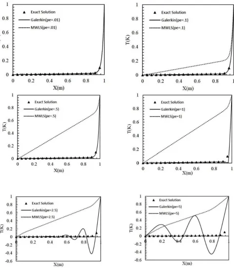
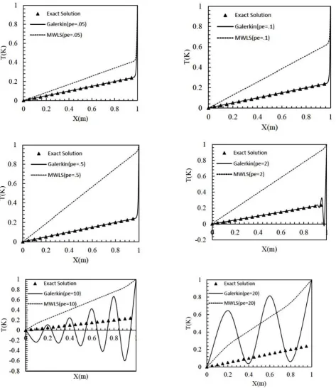
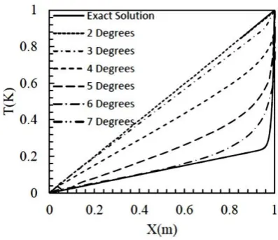
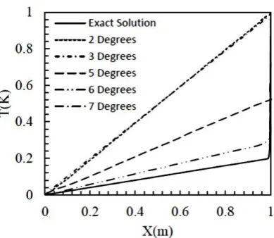
As it is obvious in Figures 1 and 2, by increasing the Peclet number, the numerical oscillations are intensified when the Galerkin method employed. Besides, when the MWLS is used, numerical solutions do not oscillate at each node but also the results are far from the exact solution. In order to eliminate these oscillations, the upward scheme is employed and also, in order to approach the the MWLS results to exact solution, thep-Version scheme can be used as far as the natural stabilization is concerned.
3.2. The upwind scheme
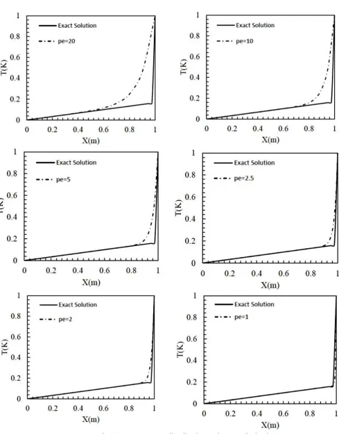
It is a common used scheme which is widely used in high Peclet numbers. In fact, with the aim of upwind scheme [44] it can be possible to overcome fluctuations caused by high convection velocity.
As can be seen in Figure 3, using upwind scheme brings about elimination of oscillations and also leads to a rapid rate of convergence.
3.3. p-Version point interpolation method
We now look at the problem set out in Eq. (3.1) with three adjacent nodesxj−1,xj and xj+1, where
the node xj is shared by two adjacent nodes. For the sake of simplicity, we apply the source term
f = 1 and consider the geometry using a uniform distance between two nodes. The shape functions of a linear basis functions are given by [45]
N1(ζ) =
1−ζ
2 (3.15)
N2(ζ) =
1 +ζ
2 (3.16)
where ζ is the normalized local coordinate. Setting Ωje = [xj, xj+1] ∈ [−1,1] and applying the
transformation between local and global coordinates, and If we assume that the field variable is Ψ , so the approximation function is as follows:
Ψh(ζ) =
1−ζ
2
Ψ1+
1 +ζ
2
Ψ2 (3.17)
Figure 1: Temperature distribution in Pe=50 and different grid Peclet numbers.
Figure 2: Temperature distribution in Pe=200 and different grid Peclet numbers.
defined the hierarchical function as [45]
Ψh(ζ) =
1−ζ
2
Ψ1+
1 +ζ
2
Ψ3+
p
X
i=2
ζi−a "
1
i!
∂iΨ
∂ζi
ζ=0 #
or in a compact form
Ψh(ζ) = N1Ψ1+N3Ψ3+
p
X
i=2
N2iΨ(2i) (3.19)
where
N1(ζ) =
1−ζ
2 , N3(ζ) = 1 +ζ
2 , N
i
2 =ζ
i−a,
1 i=even ζ i=odd Ψ
(i)
2 =
"
1
i!
∂iΨ
∂ζi
ζ=0
# (3.20)
Lagrange interpolation functions indeed are the approximation functions and we can write the fol-lowing for the temperature approximation:
Ti(ζ) = nζ X
m=1
Nm(ζ)Tim (3.21)
Substituting Nm(ζ) and rearranging the terms for the three-node parabolic case we can write the
following:
Ti(ζ) =
1−ζ
2
Ti1+
1 +ζ
2
Ti3+
ζ2−1
2
(Ti1−2Ti2+Ti3) (3.22)
If we now differentiate Eq. 3.22 with respect to ζ and evaluate these derivatives at ζ = 0 and substitute these back into Eq. 3.22, then we obtain the following for Ti(ζ):
Ti(ζ) =
1−ζ
2
Ti1+
1 +ζ
2
Ti3+
ζ2−1
2
∂2T
i
∂ζ2
ζ=0
(3.23)
Similarly, using Eq. 3.24 and substituting for Nm(ζ) and rearranging the terms for the four-node
cubic case we can write the following:
Ti(ζ) = 1−ζ2
Ti1+ 1+2ζ
Ti4+
ζ2−1 2
18
16(Ti1−Ti2 −Ti3+Ti4)
+ζ36−ζ 5416(−Ti1+ 3Ti2−3Ti3+Ti4)
(3.24)
or,
Ti(ζ) = 1−ζ2
Ti1+ 1+2ζ
Ti4+
ζ2−1 2
∂2T i ∂ζ2 ζ=0 +
ζ3−ζ 6
∂3T i ∂ζ3
ζ=0
(3.25)
3.3.1. Numerical example
In this section it is shown that how increasing the degrees of freedom between three nodes in the domain of solution can converge the solution and also, provide stability for the solution.
Figure 4: The effects of increasing degrees of freedom on temperature distribution in Pe=10 and pe=1.
Figure 5: The effects of increasing degrees of freedom on temperature distribution in Pe=20 and pe=0.5.
Figure 7: The effects of increasing degrees of freedom on temperature distribution in Pe=500 and pe=2.5.
Figure 8: The effects of increasing degrees of freedom on temperature distribution in Pe=500 and pe=10.
4. Conclusion
In this study, the convection-diffusion problem is solved in different Peclet numbers using LPIM meshless method. Various innovative methods are employed in order to eliminate the oscillations of the solution as the Peclet number increases. As shown in this study, increasing degrees of freedom provide sufficient stability for convection-dominated problems. In these cases, the scheme may also easily outperform low order stabilized methods, thanks to its high accuracy and, in many cases, exponential rate of convergence.
References
[1] P. Zhu, L.W. Zhang and K.M. Liew, Geometrically nonlinear thermo mechanical Analysis of moderately thick functionally graded plates using a local PetrovGalerkin approach with moving kriging interpolation, Compos. Struct. 107 (2014) 314–298.
[2] L.W. Zhang, Z.X. Lei, K.M. Liew and J.L. Yu, Static and dynamic of carbon nanotube Reinforced functionally graded cylindrical panels, Compos. Struct. 111 (2014) 212–205.
[3] Z.X. Lei, L.W. Zhang, K.M. Liew and J.L. Yu, Dynamic stability analysis of carbon nanotube-reinforced func-tionally graded cylindrical panels using the element-free kp-Ritz method, Compos. Struct. 113 (2014) 338–328. [4] L.W. Zhang, Z.X. Lei, K.M. Liew and J.L. Yu, Large deflection geometrically nonlinear Analysis of carbon
nanotube-reinforced functionally graded cylindrical panels, Comput. Method. Appl. MechEng. 273 (2014) 18–1. [5] Y. Cao, LQ. Yao and SC. Yi,A weighted nodal-radial point interpolation meshless method for 2D solid problems,
Eng. Anal. Bound. Elem. 39 (2014) 100–88.
[6] M.J. Peng, R.X. Li and Y.M. Cheng, Analyzing three-dimensional viscoelasticity problems via the improved element-free Galerkin(IEFG) method, Eng. Anal. Bound. Elem. 40 (2014) 113–104.
[7] M. Ebrahimnejad, N. Fallh and A.R. Khoei,New approximation functions in the meshless finite volume method for 2D elasticity problems, Eng. Anal. Bound. Elem. 46 (2014) 22–10.
[8] J.W. Yan, L.W. Zhang, K.M. Liew and L.H. He, A higher-order gradient theory for modeling of the vibration behavior of single-wall carbon nanocones, Appl. Math. Model. 38 (2014) 2960–2946.
[9] K. Kiani, A nonlocal meshless solution for flexural vibrations of double-walled carbon nanotubes, Appl. Math. Model. 234 (2014) 578–557.
[10] P.F. Guo, L.W. Zhang and K.M. Liew, Numerical analysis of generalized regularized long wave equation using the element-free kp-Ritz method, Appl. Math. Model. 240 (2014) 101–91.
[11] R.J. Cheng, L.W. Zhang and K.M. Liew,Modeling of biological population problems using the element-free kp-Ritz method, Appl. Math. Model. 227 (2014) 290–274.
[12] L.W. Zhang, Y.J. Deng and K.M. Liew, An improved element-free Galerkin method for numerical modeling of the biological population problems, Eng. Anal. Bound. Elem. 40 (2014) 188–181.
[13] K.M. Liew, Z.X. Lei, J.L. Yu and L.W. Zhang, Post buckling of carbon nanotube-reinforced functionally graded cylindrical panels under axial compression using a meshless approach, Comput. Method. Appl. Mech. Eng. 268 (2014) 18–1.
[14] L.W. Zhang, P. Zhu and K.M. Liew,Thermal buckling of functionally graded plates using a local kriging meshless method, Compos. Struct. 108 (2014) 492–472.
[15] P.W. Cleary and J.J. Monaghan, Conduction modeling using smoothed particle hydrodynamics, Comput. Phys. 148 (1999) 264–227.
[16] F. Jiang, M.S.A. Oliveira and A.C.M. Sousa, SPH simulation of transition to turbulence for planar shear flow subjected to a streamwise magnetic field, Comput. Phys. 217 (2006) 501–485.
[17] A. Khayyer, H. Gotoh and S.D. Shao,Corrected Incompressible SPH method for accurate water-surface tracking in breaking waves, Coastal. Eng. 55 (2008) 250–236.
[18] R. Xu, P. Stansby and D. Laurence,Accuracy and stability in incompressible SPH (ISPH) based on the projection method and a new approach, Comput. Phys. 228 (2009) 6725–6703.
[19] J. Fang, A. Parriaux and M. Rentschler,Improved SPH methods for simulating free surface flows of viscous fluids, Appl. Numer. Math. 71 (2009) 271–251.
[20] A. Ferrari, M. Dumbser and E.F. Toro,A new 3D parallel SPH scheme for free surface flows, Comput. Fluid. 38 (2009) 1217–1203.
[22] T.P. Fries and H.G. Matthies,A stabilized and coupled meshfree/meshbased method for the incompressible Navier-Stokes equationspart II: coupling, Comput. Method. Appl. Mech. Eng. 195 (2006) 6204–6191.
[23] T.P. Fries and H.G. Matthies,A stabilized and coupled meshfree/meshbased method for the incompressible Navier-Stokes equations-part I: stabilization, Comput. Method. Appl. Mech. Eng. 195 (2006) 6224–6205.
[24] H. Lin and S.N. Atluri,Meshless local Petrov-Galerkin (MLPG) method for convection-diffusion problems, Com-put. Model. Eng. Sci. 1 (2000) 60–45.
[25] H. Lin and S.N. Atluri, The meshless local Petrov-Galerkin(MLPG) method for solving incompressible Navier-Stokes equation, Comput. Model. Eng. Sci. 2 (2001) 142–117.
[26] G.R. Liu, Y.L. Wu and H. Ding,Meshfree weak-strong (MWS) form method and its application to incompressible flow problems, Int. J. Numer. Method. Fluid. 46 (2004) 1047–1025.
[27] C. Shu, H. Ding and K.S. Yeo,Local radial basis function-based differential quadrature method and its application to solve two-dimensional incompressible Navier-Stokes equations, Comput. Method. Appl. Mech. Eng. 192 (2003) 954–941.
[28] A. Brooks and T. Hughes,Streamline upwind PetrovGalerkin formulations for convection dominated flows with particular emphasis on the incompressible NavierStokes equations, Comput. Method. Appl. Mech. Eng. 32 (1982) 259–199.
[29] T. Hughes, L. Franca and M. Mallet, A new finite element formulation for computational fluid dynamics: I. Symmetric forms of the compressible Euler and Navier-Stokes equations and the second law of thermodynamics, Comput. Method. Appl. Mech. Eng. 54 (1986) 234–223.
[30] M. Braack and E. Burman,Local projection stabilization for the oseen problem and its interpretation as a varia-tional multiscale method, SIAM J. Numer. Anal. 43 (2006) 2566–2544.
[31] G. Matthies, P. Skrzypacz and L. Tobiska, Stabilization of local projection type applied to convection-diffusion problems with mixed boundary conditions, Electron. Trans. Numer. Anal. 32 (2006) 105–90.
[32] P. Knobloch and L. Tobiska, On the stability of finite-element discretizations of convection diffusion reaction equations, IMA J. Numer. Anal. 31 (2011) 164–147.
[33] R. Codina and J. Blasco, Analysis of a stabilized finite element approximation of the transient convection-diffusionreaction equation using orthogonal subscales, Comput. Vis. Sci. 4 (2002) 174–167.
[34] I. Harari and T.J.R. Hughes, Stabilized finite element methods for steady advection-diffusion with production, Comput. Method. Appl. Mech. Eng. 115 (1994) 191–165.
[35] T.J.R. Hughes, Multiscale phenomena: Green’s functions, the Dirichlet-to-Neumann formulation, subgrid scale models, bubbles and the origins of stabilized methods, Comput. Method. Appl. Mech. Eng. 127 (1995) 401–387. [36] T.J.R. Hughes and G.M. Hulbert, Large eddy simulation and the variational multiscale method, Comput. Vis.
Sci. 3 (2000) 59–47.
[37] T.J.R. Hughes and G. Sangalli, Variational multiscale analysis: the final-scale Greens functions, projection, optimization, localization and stabilized methods, SIAM J. Numer. Anal. 45 (2007) 557–539.
[38] A. Quarteroni,Numerical Models for Differential Problems, Springer Science & Business Media. 2 (2010). [39] L. Tobiska, Analysis of a new stabilized higher order finite element method for advection diffusion equations,
Comput Methods Appl Mech Eng. 196 (2006) 550–538.
[40] H.G. Roos, M. Stynes and L. Tobiska,Robust Numerical Methods for Singularly Perturbed Differential Equations, Appl. Math. 24 (2012).
[41] G. Lube and G. Rapin,Residual-based stabilized higher-order FEM for advection-dominated problems, Comput. Method. Appl. Mech. Eng. 195 (2006) 4138–4124.
[42] J. Donea and A. Huerta,Finite Element Methods for Flow Problems, John Wiley, 2003.
[43] S.C. Wu, G.R. Liu, X.Y. Cui, T.T. Nguyen and G.Y. Zhang,An edge-based smoothed point interpolation method (ES-PIM) for heat transfer analysis of rapid manufacturing system, Int. J. Heat Mass Transf. 53 (2010) 1950–1938. [44] V. Patankar,Numerical heat transfer and fluid flow, McGRAW-HILL book, 1980.