DOCTORAL SCHOOL IN
PSYCHOLOGICAL SCIENCES AND EDUCATION
XXVIII CYCLE
Doctoral Dissertation
Measuring real-time dynamics underlying online
rating processes:
Models, methods, applications
Phd Scholar
Antonio Calcagnì
Advisor prof. Luigi Lombardi
Head of the doctoral school prof.ssa Paola Venuti
cielo? Chi avrebbe conosciuto il tuo volere, se tu non gli avessi dato la sapienza e dall’alto non gli avessi inviato il tuo santo spirito? Così vennero raddrizzati i sentieri di chi è sulla terra; gli uomini furono istruiti in ciò che ti è gradito [...].”
Sapienza 9, 16-18
elaborato emerge dall’incontro fruttuoso con altre persone che coi loro saperi hanno collaborato a rendere il tutto un composito omogeneo e strutturato al suo interno. È perciò atto piacevolmente dovuto quello di esprimere la mia gratitudine verso coloro che mi hanno guidato ed accompagnato in questo viaggio volto ad approfondire una piccola parte del vasto sapere scientifico, all’interno di un progressivo percorso di studio e conoscenza delle pratiche che la concorrono a formare.
Nella consapevolezza che le parole sono insufficienti ad esprimere i più profondi vissuti, un primo sincero ringraziamento è rivolto al prof. Luigi Lombardi che con paziente e costante presenza mi ha traghettato verso l’apprendimento di quegli uten-sili necessari alla buona pratica della ricerca scientifica. Come un vasaio fa con l’argilla, ha progressivamente favorito la mia crescita scientifica e personale sino alla matu-razione oggi raggiunta, entro un processo che ancora prosegue e proseguirà. Come un “operaio” ho appreso quest’umile mestiere presso la sua “bottega” di esperienza e saggezza. La mia attuale maturazione è primariamente frutto dell’intenso lavoro fatto con lui in questi anni.
Un secondo ringraziamento è per coloro che più avanti in questo percorso hanno sa-puto donarmi il loro tempo ma anche la loro amicizia. In particolare, Lorenzo, Si-mone e Mara che nelle diversità dei loro carismi hanno permesso la realizzazione di alcuni progetti insieme. Sentimento di gratitudine anche per i miei amici e colleghi Francesco, Janet, Andrea, Yagmur e Mauro insieme ai quali ho condiviso questo per-corso.
Con viva gratitudine non posso non ricordare tutti i docenti di questa Scuola che hanno donato il loro tempo nell’organizzare ed incoraggiare le attività di formazione. In particolare, la prof.ssa Paola Venuti che in qualità di coordinatrice ci ha guidato in questo percorso di crescita personale e professionale.
Un ultimo ringraziamento è per Martina che con la sua saggezza di donna mi ha ac-compagnato nelle fasi finali di questo percorso. Coniugando cuore e ragione con la dovuta semplicità dell’abbandono provvidenziale, mi ha supportato ed incoraggiato amorevolmente nell’affrontare le fatiche del crescere e del maturare.
Introduction 1
MODELS, METHODS, INSTRUMENTS 3
1 Dynamic Fuzzy Rating Tracker (DYFRAT): a novel methodology for modeling real time
dynamic cognitive processes in rating scales 7
1.1 Introduction . . . 7
1.2 Currently used methods for fuzzy ratings . . . 10
1.2.1 Fuzzy conversion scales . . . 10
1.2.2 Fuzzy rating scales . . . 11
1.3 Dynamic Fuzzy Rating Tracker: theory . . . 13
1.4 Dynamic Fuzzy Rating Tracker: methodology . . . 15
1.4.1 Data-capturing procedure . . . 15
1.4.2 Data representation . . . 16
1.4.3 Data modeling . . . 17
1.4.4 Summary measures . . . 22
1.5 Dynamic Fuzzy Rating Tracker: implementation . . . 24
1.6 Illustrative examples . . . 25
1.6.1 Rating responses and moral dilemma . . . 25
1.6.2 Self-report behaviors in reckless driving . . . 29
1.6.3 Outlier detection analysis . . . 34
1.7 Final remarks . . . 36
1.7.1 Limitations . . . 37
1.7.2 Conclusions . . . 38
2 Representing the dynamics of rating responses: An activation function approach 39 2.1 Introduction . . . 39
2.2 Rating evaluations as dynamic activation processes . . . 41
2.2.1 Temporal and activation state measures . . . 42
2.3 Methodology . . . 47
2.3.1 Data representation . . . 47
Spatio-temporal data . . . 47
From spatio-temporal data to functional data . . . 48
2.3.2 Data modeling and parsing . . . 50
2.4 Illustrative examples . . . 52
2.4.1 Rating responses and moral dilemma . . . 52
3 A simple information theoretic approach for modeling spatial data from mouse tracker
methodology 67
3.1 Introduction . . . 67
3.2 Descriptive geometric approach: a brief overview . . . 71
3.2.1 General context and motivation . . . 71
3.2.2 Procedures and data analysis . . . 72
3.2.3 Some critical issues . . . 74
3.3 Information theoretic approach to spatial information . . . 76
3.3.1 General context and motivation . . . 76
3.3.2 InTMT approach . . . 77
Data modeling . . . 77
Data analysis . . . 80
3.4 Some exemplary applications . . . 83
3.5 Conclusions . . . 89
STATISTICAL TECHNIQUES 91 4 Non-convex fuzzy data and fuzzy statistics. A first descriptive approach to data analysis 95 4.1 Introduction . . . 95
4.2 Non-convex fuzzy numbers: a computational proposal . . . 97
4.2.1 Convex fuzzy sets and LR fuzzy numbers . . . 97
4.2.2 Non-convex fuzzy sets and non-convex fuzzy numbers . . . 99
4.3 A Fuzzy regression model for 2-mode fuzzy numbers: thecrisp-input/fuzzy-output case . . . 102
4.3.1 Model and data analysis . . . 103
4.3.2 Parameters estimation: an unconstrained version . . . 104
Parameters estimation forM1 . . . 104
Parameters estimation forM2 . . . 106
4.3.3 Properties of the model . . . 106
4.3.4 Goodness of fit indices for the model . . . 107
4.3.5 Some remarks . . . 109
About the model complexity issue. . . 109
About the model representation issue. . . 109
About the algorithmic issue. . . 109
4.4 Applications . . . 110
4.4.1 Example 1: Response Times and Moral Dilemma . . . 110
4.4.2 Example 2: Private Consumption and Perceived Satisfaction . . . 113
4.4.3 Example 3: Unemployment and Employment rates . . . 116
4.4.4 Example 4: Degenerate non-convex fuzzy data - triangular case . . . 118
4.4.5 Example 5: Degenerate non-convex fuzzy data - trapezoidal case . . . 119
5.1 Introduction . . . 125
5.2 Non-convex fuzzy component analysis (NCFCA) . . . 127
5.2.1 Model and data analysis . . . 128
5.2.2 Parameters estimation . . . 129
5.2.3 Data interpretation and visualization . . . 133
Data pre-treatment . . . 133
Rotation ofΓb . . . 134
Model evaluation . . . 135
Score plot . . . 136
5.3 Applications . . . 137
5.3.1 Example 1: psychological assessment of worry . . . 137
5.3.2 Example 2: Self perception of professional roles . . . 140
5.3.3 Example 3: welfare and productivity of Italian regions . . . 143
5.4 Conclusion and further perspectives . . . 145
6 Multiple mediation analysis for interval-valued data 147 6.1 Introduction . . . 147
6.2 Interval-valued data . . . 150
6.2.1 Introduction and examples of application . . . 150
6.2.2 Formal definitions . . . 152
6.2.3 Centre-range parametrization . . . 153
6.3 Interval mediation analysis . . . 154
6.3.1 General context and motivation . . . 154
6.3.2 The IMedA model . . . 155
6.4 Data analysis . . . 156
6.4.1 Parameters estimation . . . 156
6.4.2 Goodness-of-fit indices . . . 157
6.5 Analysis of effects . . . 157
6.5.1 Decomposition of effects . . . 157
6.5.2 Evaluating the size of the effects . . . 159
6.6 Simulation study . . . 161
6.6.1 Design and procedure . . . 162
6.6.2 Outcome measures . . . 163
6.6.3 Results . . . 164
6.6.4 Further analysis and results . . . 164
6.7 Empirical examples . . . 166
6.7.1 Role and work-related burnout . . . 166
6.7.2 Beauty and usability in HCI perspective . . . 168
6.8 Conclusions . . . 173
Bibliography 181
This thesis collects a set of research articles and working papers produced during my doctoral program. Overall, they refer to:
(i) the general problem of collecting measures for the dynamic processes underlying human rating tasks (section Models, methods, instruments)
(ii) the proposal of new statistical methods to analyse data structures aris-ing from the dynamic rataris-ing measurements (section Statistical tech-niques).
The sectionModels, methods, instrumentscontains three chapters on models and methods designed to represent the dynamics of rating evaluations to-gether with some relevant applications. In particular, the latter refer to two different contexts, namely Likert-type questionnaires (Chapters 1 and 2) and two-choice decision making (Chapter 3). Finally, the section also de-scribes two new measurement instruments for dynamic ratings, DYFRAT (Chapter 1) and DYFRAS (Chapter 2). In a similar way, the section Statis-tical techniques contains three works on novel statistical methodologies to run data analysis in the context of “structured data”, namely fuzzy num-bers (Chapters 4 and 5) and interval-valued data (Chapter 6). The justifica-tion for structured-data comes directly from the treatment of the dynamic rating components in the sense that such a kind of data can offer a simple and flexible formal representation to model the information related to the rating properties.
Traditionally, rating objects like attitudes, opinions, and subjective eval-uations have been investigated by means of Likert-type questionnaires
and/or similar methodologies (e.g., see: Aiken, 1996). In this context, the extracted information have been usually codified in terms of simple and discrete numerical representations (i.e., final discrete responses and even-tually their associated response times). The standard assumption here is that these standard observable measures are “end products” of the entire process of rating and, as such, can be used as indicators of the raters’ over-all performance. In this way, the dynamics underlying final rating mea-sures are clearly not detected with the consequence of loss of information. Although this issue is not completely new in the psychological tradition (e.g., see: Anderson, 1981; Tourangeau and Rasinski, 1988; Smith and De-Coster, 2000; Link, Townsend, and Ashby, 1985), over the recent years it is becoming popular again (e.g., see: Rosenbaum, 2005; Dale, Hindy, and Spivey, 2006). This can be also noticed in other scientific traditions (e.g., see the recent methods employed in neuroscientific investigations such as the GPFA method or the so-called trial-by-trial analysis - Byron et al., 2009; Delorme and Makeig, 2004). In this respect, studying the dynamics at the base of the rating mechanisms could give us a pragmatical but still useful window on how human evaluations, opinion, and attitude may arise.
Dynamic Fuzzy Rating Tracker
(DYFRAT): a novel methodology for
modeling real time dynamic cognitive
processes in rating scales
The content of the chapter has been previously published as: Calcagnì, A., & Lombardi, L. (2014). Dynamic Fuzzy Rating Tracker (DYFRAT): a novel methodology for modeling real-time dynamic cognitive processes in rating scales.Applied soft computing, 24, 948-961.
1.1
Introduction
In many empirical research areas such as, for instance, psychology, soci-ology, organizational and management sciences, marketing, and epidemi-ology, rating scales represent a widely used, simple and flexible tool for measuring attitudes, opinions, and subjective preferences (Göb, McCollin, and Ramalhoto, 2007; Miller and Salkind, 2002; Aiken, 1996; Pettit, 2002). Let us assume that we are interested in measuring a person’s degree of happiness. We could do this in a number of different ways, but one direct and efficient approach would be simply to ask the person, ’How happy are you?’ and require them evaluate themselves on a Likert-type rating scale, ranging from ’very unhappy’ to ’very happy’. Rating scales typi-cally consists of a variable to be measured (e.g., ’happiness’) and a set of anchor points from which the rater selects the most appropriate descrip-tion (e.g., very unhappy, moderately unhappy, neither, moderately happy,
very happy). One widely used type of rating scale is the so-called numeri-calscale, where the anchor points either explicitly or implicitly are defined numerically (e.g., 1: low, 2: average, 3: high). Like checklists, rating scales are used for a wide variety of assessment purposes. For example, rating scales can be used to have one individual evaluate another, for example, when a physician might asses a patient as to degree of obesity, but the rat-ing scales can also be applied as self-report measures. Unlike other types of ratings, self-report scales require the person provide a direct and ex-plicit rating of their own behavior/opinion/preference, etc. Of course, the main assumption behind self-report measures is that individuals are in the best position to report their own opinion in a direct and transpar-ent way. The great diffusion and success of rating scales are mainly due to the following major reasons that are all well documented in the litera-ture: (1) rating scales can be administered to large groups of respondents at one single setting; (2) they can be administered under conditions that guarantee anonymity; (3) they allow the rater to proceed at their own pace; (4) they present uniformity of procedure; (5) they allow for great flexibility - for example, take-home questionnaires; and (6) the results are more amenable to statistical analyses (in particular for numerical scales) (Domino and Domino, 2006).
therefore, the associated self-report evaluations could be definitively bi-ased (e.g., Furnham, 1986). Finally, another important limitation pertains the idea that what is being reported using rating evaluations is something that allows us to objectively explain and describe a person’s behavior. However, several psychologists argue that such assumption is, in prin-ciple, ill-posed and that what we really need, instead, is to directly focus on the observable behavior involved in the process of rating (e.g., Golfried and Kent, 1972).
In order to overcome the limitations of standard rating scales, some re-searchers have applied fuzzy set theory (FST) to directly modeling impre-cise features of human rating evaluations (Sáa et al., 2013; Li, 2012). In particular, in the rating scale problem, FST has been mainly used in two different contexts: i) for modeling data obtained by means of standard rating scales (fuzzy conversion scales) or ii) for directly quantifying empir-ical evaluations using fuzzy rating scales. In the first case, FST is applied a-posteriori as a procedure for converting standard rating data into fuzzy data (i.e., raters express their judgements using a traditional rating scale which is subsequently converted into a fuzzy structure). By contrast, in the second case, FST is applied a-priori as a general interface for directly capturing fuzzy rating data (i.e. raters give their evaluations by means of computerized tools that allow to directly use fuzzy sets in place of crisp numbers).
respect, DYFRAT is a formal procedure that explicitly focuses on the be-havioral dynamics of rating and provides a continuous on-line measure of the cognitive aspects involved in this process.
The remainder of this chapter is organized as follows. In the second sec-tion we describe a comprehensive survey of the state-of-the-art of FST applications in human rating problems. In the third and fourth sections we present our new methodology. In the fifth section we describe a first computerized implementation of DYFRAT system. In the sixth section we show some empirical applications of DYFRAT to real data, whereas in the seventh section we conclude this chapter by providing some final com-ments.
1.2
Currently used methods for fuzzy ratings
1.2.1 Fuzzy conversion scales
Fuzzy conversion scales (FCS) are computational procedures based on a fuzzy system which convert standard crisp rating data into a set of fuzzy data. Figure 1.1a shows a graphical representation of the rationale under-lying the FCS approach. In general, two perspectives can be adopted to derive the conversion scale procedure from crisp rating data: i) an expert-based approach and ii) an empirically-expert-based approach. In the first per-spective, a researcher (a-priori) sets the main features of the fuzzy vari-ables (the number and shape of fuzzy sets, their overlapping degrees, etc.) as well as some properties of the fuzzy system used in the conversion process (input and output space definition, implication rules, implication surface, etc). In the second approach, the fuzzy variables, are obtained us-ing suitable statistical or data-minus-ing procedures applied on the original crisp data (e.g., fuzzy clustering, histogram based methods, probability-possibility transformations).
airline companies (Chang and Yeh, 2002), Chan and Kao analysed cus-tomers’satisfaction (Chan, Kao, and Wu, 1999), Benítez et al. proposed a FST based method to measure hotels quality (Benítez, Martín, and Román, 2007), Lalla et al. developed a system for teaching activity evaluations (Lalla, Facchinetti, and Mastroleo, 2005), Costa et al. proposed an appli-cation for perception of disability evaluation (Costa et al., 2004), Li devel-oped a novel type of fuzzy Likert scale (Li, 2012), Moon et al. described a system for ranking candidates in military organizations (Moon, Lee, and Lim, 2010), and Chen et al. proposed a fuzzy approach for selecting environment-watershed plans (Chen et al., 2011).
However, fuzzy conversion scales are also characterized by some limita-tions which are related to their general definition of fuzzy variables. For example, aspects such as the number or type of fuzzy sets and the amount of overlap between consecutive fuzzy sets in the scale, represent all sensi-tive steps in the scale construction process. Moreover, the realization of the conversion procedure, usually implemented by means of specific fuzzy systems, is generally not a trivial task as it requires several delicate phases (e.g., evaluation of the uniqueness of the final fuzzy representation, mea-surement of the overall goodness-of-fit). In general, although the adoption of the empirically-based methodology may overcome some of the draw-backs of the expert-based approach (Ciavolino, Salvatore, and Calcagnì, 2013; Medasani, Kim, and Krishnapuram, 1998), FSC still inherits some of the limitations of standard rating scales, such as for example, the problem of selecting extreme categories in the scale and, more importantly, the fact that this methodology cannot provide any information about the underly-ing dynamics of ratunderly-ing.
1.2.2 Fuzzy rating scales
Strongly
Disagree Disagree Agree
Strongly Agree
1 2 3 4
0.2 0.4 0.6 0.8 1.0
Fuzzification Procedure
(1) (2) (3) (4)
Traditional Ordinal Scale
Fuzzy Variable
Strongly
Disagree Disagree Agree Strongly
Agree
(A)General diagram for FCS
Strongly Disagree
Strongly Agree
Strongly Disagree
Strongly Agree
Strongly Disagree
Strongly Agree
Strongly Disagree
Strongly Agree
(i) First step
(ii) Second step
(iii) Third step
Final Fuzzy Response
(B)General diagram for FRS
FIGURE1.1: Graphical comparison between FCS and FRS
the evaluation of psychological constructs (Costas, Maranon, and Cabr-era, 1994), finally, Gil et al. described a free fuzzy-numbered response for-mat questionnaire and compared it with standard rating scales (Gil and González-Rodríguez, 2012).
However, the application of fuzzy scaling methods can also be problem-atic. In particular, FRS can lack some ecological validity as subjects must follow specific training periods for learning how the instrument exactly works, what the concept of fuzziness is and, above all, how it can be used to directly express their judgements or evaluations. Moreover, FRS can also be criticized because this technique asks respondents to provide in-formation that may seem difficult or even tricky to them. For this reason, the basic assumption underpinning FRS, namely that human raters are able to explicitly express the fuzziness of their judgements or evaluations by means of fuzzy sets, could be questionable. Therefore, due to the high complexity of the rating procedure, we cannot exclude that in some situ-ations data collected using the FRS framework could be distorted or even meaningless (Howard and Dailey, 1979; Furnham and Henderson, 1982; Windschitl and Wells, 1996).
1.3
Dynamic Fuzzy Rating Tracker: theory
1.4
Dynamic Fuzzy Rating Tracker: methodology
DYFRAT consists of a data-capturing procedure which implements a MTM
based computerized interface for collecting the motor and temporal com-ponents in the process of rating and a data-modeling procedure which pro-vides a fuzzy model for the recorded information.
1.4.1 Data-capturing procedure
configuration yields the largest degrees of freedom for mouse-movement recordings (Johnson et al., 2012). However, unlike genuine circular scales, a pseudo-circular representation still preserves the ordinal property be-tween consecutive anchor points in the scale as it shows a visible break-point between the first level and the last level of the rating scale. The pro-posed configuration can be considered as a standard linear scale which has been bent in order to take into account the properties of both standard linear scales as well as circular ones.
What is your overall satisfaction with our product?
CONTINUE
CONTINUE
Strongly Disagree
Agree
Disag
ree
S
tr
ongly A
g
ree
(A)General diagram of the pro-posed scale
What is your overall satisfaction with our product?
CONTINUE
CONTINUE
Strongly Disagree
Agree
Disag
ree
S
tr
ongly A
g
ree
What is your overall satisfaction?
CONTINUE
CONTINUE
Strongly Disagree
Agree
Disag
ree
S
tr
ongly A
g
ree
FIRST ITEM
SECOND ITEM
time
(B)Temporal diagram for two or more questionnaire items
FIGURE1.2: DYFRAT: graphical schematization of the interface for data-capturing procedure
1.4.2 Data representation
The collected data are represented by an I × J array D, that is to say, I
observations (raters) containingJ structured measures (rater’s measures). The entrydij ofDdenotes ageneralized rating measure defined as:
dij = hzij, tij,piji, i = 1, . . . , I;j = 1, . . . , J
are Nij ×1vectors of Cartesian coordinates associated to the streaming of the x-y coordinates of the computer mouse movements (movements path of lengthNij) .
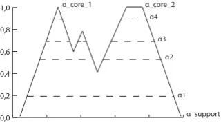
The main idea is to construct a new I × J array De, called the fuzzy data array ofD, by transforming each generalized rating measuredij into a cor-responding fuzzy set deij that expresses the overall fuzziness of the rating score associated with the(i, j)response. Therefore, according to our ratio-nale, we consider mouse-movements and response times as two particular sources of uncertainty, namely spatial uncertainty and temporal uncertainty. By contrast, the ordinal crisp response is understood as the final output of the dynamic decision process. A two-step procedure is used to derive the final fuzzy representationdeij fromdij. In the first step, we model (in an in-dependent fashion) the spatial uncertainty and the temporal uncertainty. In the second step, we provide the final fuzzy model representation,deij, by integrating these two sources of uncertainty. In particular, the rater’s final response is captured by the core core( ˜dij) of the fuzzy set d˜ij, the spatial uncertainty is described by the support supp( ˜dij), whereas the temporal uncertainty is modelled by the membership functionµd˜ij.1
1.4.3 Data modeling
In what follows we describe the two-step procedure to derive the final fuzzy set deij according to the DYFRAT framework.
First step. In the first stage of the fuzzy modeling procedure, a fuzzy setpeij representing the spatial uncertainty is constructed from the generalized rating measure dij. In particular, to derive peij we first remove eventual imprecision due to hand motor controls and/or computer mouse adjust-ments. To this end, the x-y coordinates in pij that are located near to the starting point (the center of the scale), the points that are recorded in the
breakpoint area, and those ones that are beyond the border of the pseudo-circular scale, are all removed by applying a predefined filter which de-fines the area for acceptable x-y coordinates. The refined pij is next trans-formed into a vectormcij of angles (expressed in radians) by using the well-known atan2 function, namely mcij = atan2(pij).2 The fuzzy setpeij is con-structed from the histogram of the radian measures collected in mcij. We callpeij the spatial fuzzy set ofdij. There are several procedures that can be adopted to derive fuzzy sets from data histograms (Medasani, Kim, and Krishnapuram, 1998). In the DYFRAT approach we adopted a heuristic procedure based on the particle swarm optimization (PSO) algorithm (Poli, Kennedy, and Blackwell, 2007). The PSO algorithm looks for the best fuzzy set that maximizes the total entropy with respect to the data his-togram (Nieradka and Butkiewicz, 2007; Cheng and Chen, 1997; Li and Li, 2008). In particular, for the maximization algorithm we used the well known total fuzzy entropy measure proposed by De Luca and Termini (De Luca and Termini, 1972). Several convex as well as non-convex fuzzy sets can be used for representing a histogram (e.g., triangular, trapezoidal, gaussian. See: Ross, 2009; Calcagnì, Lombardi, and Pascali, 2013). How-ever, for the sake of simplicity, in this contribution we opted for the sim-plest triangular format which is associated to the well-known LR repre-sentation (Dubois et al., 1988). In this respect, the triangular membership function may also be useful when one wants to analyze these variables on the basis of some widely used fuzzy statistical techniques (e.g., Taheri, 2003; Coppi, Gil, and Kiers, 2006). Some examples of fuzzy sets derived from the radian histograms are shown in figure 1.3. In particular, figure 1.3a shows a pattern of movements characterized by a modest spatial un-certainty which corresponds to a fuzzy set with a narrow support. By contrast, figure 1.3b shows a pattern of movements in which the spatial
2Theatan2(y, x)function is the arc tangent of the two variablesxandyand uses the signs of both arguments in
uncertainty is related to the rater’s choice between two possible alterna-tives. Note that in this second configuration the associated fuzzy set has now a wider support and its core has shifted toward the right side. Finally, figure 1.3c presents an interesting pattern in which the spatial uncertainty is related to the choice among three distinct options. This last configura-tion shows the largest support for the derived fuzzy set.
1 2 3 4 5
0.2 0.4 0.6 0.8 1.0
1 2 3 4 5
0.2 0.4 0.6 0.8 1.0
-200 -100 10 0 200 -200 -100 100 200 2 3 4 5 1
(A)Spatial uncertainty related to a simple direct response (final response = 1)
1 2 3 4 5
0.2 0.4 0.6 0.8 1.0
1 2 3 4 5
0.1 0.15 0.20 0.25 0.30
-200 -100 10 0 200 -200 -100 100 200 2 3 4 5 1
(B)Spatial uncertainty related to the choice between two alternatives (final response = 1)
1 2 3 4 5
0.2 0.4 0.6 0.8 1.0
1 2 3 4 5
0.01 0.04 0.07 0.10 0.15
-200 -100 10 0 200
-200 -100 100 200 2 3 4 5 1
(C)Spatial uncertainty related to the choice among three alternatives (final response = 3)
FIGURE 1.3: Three types of empirical mouse movements with the correspondent histograms and fuzzy sets. Note that, the continuous black circle represents the original scale, the dashed red ones represents the filters whereas the blue points indicate the recorded mouse movements. The ordinal numbers codify the anchor points of the scale (e.g., Strongly Disagree = 1, Disagree = 2, Neither = 3, Agree = 4, Strongly Agree = 5) that are simply juxtaposed on the scale of radians for the sake of exposition.
according to the following conditional equations:
µd˜ij(x) =
0.5−(22γij−1)·[0.5−µ
˜
pij(x)]
2γij,
b
F(tij)>Fb(¯tj) and 0≤µp˜ij(x)≤0.5
1−(20.5ωij)·[1−µ
˜
pij(x)]
0.5ωij,
b
F(tij)>Fb(¯tj) and 0.5< µp˜ij(x)≤1
µp˜ij(x)
νij
, Fb(tij)<Fb(¯tj) and 0≤µp˜ij(x)≤1 µp˜ij(x), Fb(tij) =Fb(¯tj) and 0≤µp˜ij(x)≤1
(1.1)
with
γij = λijFb(tij), ωij =
1
γij
, and νij =
1
2Fb(tij)
and whereFbdenotes the empirical cumulative distribution function of the response times sample tj = (t1j, t2j, . . . , tIj) associated to item j whereas
¯
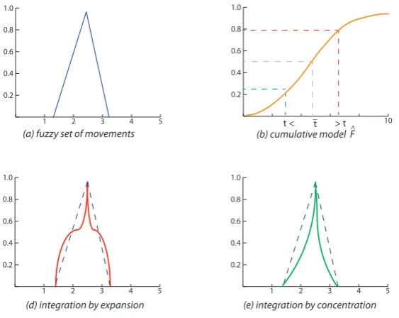
tj indicates the sample mean of tj. The first and the second lines of for-mula 1.1 act as an expansion modifier which increases the overall uncer-tainty represented in the original spatial fuzzy set peij. In particular, if the recorded timetij for raterito itemj is larger than the corresponding aver-age time tj, thenpeij is nonlinearly expanded according to a model param-eter γij which, in turn, depends on the cumulative density value oftij and the shape parameterλij3. By contrast, the third line of formula 1.1 acts as a
concentrationmodifier which decreases the overall uncertainty represented in peij. In particular, if the recorded time tij for rater i to item j is smaller than the corresponding average sample timetj, thenpeij is nonlinearly con-centrated according to a shape parameter νij which is inversely related to the cumulative density value of tij. Finally, the fourth line of formula 1.1 represents the fuzzy set when the observed response time tij is perfectly equivalent to the average response time for itemj. In this last case the new fuzzy set deij simply boils down to the original spatial fuzzy set
e
pij. Note that, that the third line of formula 1.1 corresponds to the well-known lin-guistic hedge called concentration which allows to reduce the fuzziness of the set. Similarly, the first and second lines of formula 1.1 is inspired by the
3λ
ij is a coefficient which maximizes the overall fuzziness of the set. Given the fuzzy set of movementspeij, the
best value forλijis obtained by adopting an iterative optimization algorithm which maximizes the Kaufmann index
Zadeh’s linguist hedge called intensification (Huynh, Ho, and Nakamori, 2002) which allows to intensify (to expand) the fuzziness of the set. In our approach the expansion was created ad-hoc in order to obtain an in-creasing level of fuzziness for the set. More precisely, if µ
e
pij(x) ≤ 0.5 we expanded the base of the set, otherwise we reduced the peak of the set. Figure 1.4 shows a graphical summary of this expansion/concentration transformation.
1 2 3 4 5
0.2 0.4 0.6 0.8 1.0
(a) fuzzy set of movements
10 0.2
0.4 0.6 0.8 1.0
(b) cumulative model F
1 2 3 4 5
0.2 0.4 0.6 0.8 1.0
(d) integration by expansion
1 2 3 4 5
0.2 0.4 0.6 0.8 1.0
(e) integration by concentration ^ _ t t < > t
FIGURE1.4: Graphical schematization for the integration process
However, in the DYFRAT context we stress that the equations used for the integration between movement patterns and response times are only used according to a descriptive fashion and, therefore, they cannot be conceived as linguistic hedges in a strict fuzzy logic sense. Moreover, we preferred to develop a novel fuzzy modifier according to a statistically oriented per-spective (e.g., using the cumulative distribution function for the response times and the observed average response time for the item) because we were interested in providing a rational procedure to transform a fuzzy set according to observed distributional data (empirical distribution of times and empirical distribution of movements).
Haidt, 2002). In particular, according to these theories intuitive judge-ments or evaluations occur quickly, effortlessly, and almost automatically, such that the final responses (but not necessarily the underlying processes) are accessible to consciousness. By contrast, more elaborated or conflict-ing reasonconflict-ings occur more slowly, require some additional efforts, and presumably involve some more steps that are directly accessible to con-sciousness. The latter type of responses are usually characterized by a much larger level of uncertainty. With our model we tried to capture this psychological intuition according to a purely descriptive representation.
1.4.4 Summary measures
Fuzzy summary measures can play a relevant role in highlighting impor-tant properties of the final fuzzy set deij. In the DYFRAT framework we implemented the following basic and well known fuzzy set measures:
• Kaufmann index (Kaufmann and Swanson, 1975):
K(deij) =
2
card(deij)
·X
x
|µ
e
dij(x)−δ(x)| (1.2)
with δ(x) =
1, ifµ
e
dij(x) ≥0.5
0, ifµ
e
dij(x) < 0.5
and where card(.) is the cardinality of the final fuzzy set deij.
• Fuzzy entropyDe Luca and Termini, 1972:
H(deij) = − X
x
[µ
e
dij(x) log(µdeij(x))]−[(1−µdeij(x)) log(1−µdeij(x))] (1.3)
• COG based Fuzzy centroidRoss, 2009:
CR(deij) =
X
x
x·µ
e dij(x)
·
X
x
µ
e dij(x)
−1
• Total spread (or length of the fuzzy set support):
T S(deij) =max(supp(deij))−min(supp(deij)) (1.5)
In addition, we also considered a new simple fuzzy measure, called the intensification index, derived from the fuzzy entropy measure. In particular, the intensification index is defined as follows:
HR(deij, e
pij) =
H(deij)−H(peij)
H(peij)
(1.6)
where H(peij) and H(deij) indicate the entropies associated to the spatial and final fuzzy sets, respectively. Values of HR(deij,
e
pij) < 0 indicate the quantity of information which is subtracted by concentration from the spa-tial fuzzy set peij, whereas values of HR(deij,peij) > 0 indicate the quantity of information which is added by expansion on peij.
One important comment is in order concerning the defuzzification mea-sures adopted for the final fuzzy set. In general, several meamea-sures can be selected to perform the defuzzification of a fuzzy set (Roychowdhury and Pedrycz, 2001). In this first implementation of the DYFRAT system we opted for a COG based index because of its simplicity and high flexibil-ity. In particular, the COG centroid is a measure which fully takes into account the integration between movements and times. More specifically, unlike other defuzzification measures (e.g., first of maximum FoM, last of maximum LoM, mean of maxima MEoM, etc.), the COG index also con-siders the weighted information provided by the membership function of the final fuzzy set.
who use the computer-mouse in an improper way (outliers for mouse-movements). Similarly, the intensification index can be used for detecting anomalous subjects with lower or greater response times (outliers for re-sponse times). We will provide some examples of indices applications in the sixth section of the manuscript.
1.5
Dynamic Fuzzy Rating Tracker: implementation
Data-modeling procedure. The second application consists of a GUI-based system developed in Matlab for Windows, OSX and Unix systems that im-plements the modeling steps of the DYFRAT methodology (see Figure 1.5-b). All the features involved in the analysis (e.g., type of filters, histogram of movements, PSO parameters) can be set by the user. Moreover, differ-ent types of analysis (e.g., subject-by-subject, item-by-item, global) with different characteristics (temporized or static analysis) can be selected. Finally, the application provides a single output containing the main re-sults of the analysis. These are organized by means of two-way (two-dimensional matrices) as well as three-way array structures (three dimen-sional matrices).
1.6
Illustrative examples
By way of illustration we consider three simple applications using the DYFRAT methodology. The first example is about the evaluation of a well known cognitive problem in decision making. The second application considers data about rash driving behaviors among young people aged 18-26. Finally, the third application illustrates how one can perform an outlier detection analysis using the DYFRAT framework.
1.6.1 Rating responses and moral dilemma
General context and motivation. In cognitive decision making (Greene and Haidt, 2002; Haidt, 2001), moral judgements and dilemmas are relevant phenomena characterized by high levels of uncertainty in individuals re-sponses. In this application, we used a moral dilemma based on the well-known trolley scenario (Greene and Haidt, 2002; Haidt, 2001; McGuire et al., 2009):
(A)Interface for data-capturing developed in Processing
(B)Interface for data-modeling developed in Matlab
FIGURE1.5: Screen-shots from DYFRAT implementation
the final judgment (but not the underlying process) is accessible to con-sciousness, whereas moral reasoning occurs more slowly, requires some effort, and involves at least some steps that are accessible to conscious-ness. In this first example, we studied the relationship between response uncertainty, as measured by the Kaufmann index of the final fuzzy set, and moral judgement as represented by the centroid of the same fuzzy set. We expect that the individuals who show a very strong disagreement with the action described in the trolley scenario (moral intuition raters) will be characterized by very fast responses with low levels of uncertainty. By contrast, those who are characterized by a more moral thinking attitude (moral reasoning raters) will show less extreme responses with larger val-ues of uncertainty. Because the trolley scenario may activate not necessar-ily conscious underlying processes in the rater, we believe that DYFRAT can represent an ideal methodology for testing this hypothesis.
Data-analysis and results. The trolley dilemma was administered to a group of students (I = 103, 47 males, age 18-23 : 70.87%, age 24-27 : 19.42%, age 28-36 : 2.91%, age ≥ 37 : 3.88%) from the University of Trento (Italy) and the responses were collected using the DYFRAT graphical interface. In particular, participants used a pseudo-circular scale with five response levels (strongly disag.=1, disag.=2, neither=3, agree=4, strongly agree=5). Figure 1.6 shows two empirical patterns of mouse movements with the final fuzzy sets. In particular, Figure 1.6a represents an empirical pattern with a low uncertainty/fuzziness, by contrast Figure 1.6b shows a pattern with a higher level of uncertainty. Table 1.1 reports some results for the two selected subjects.
Subj. z CR t K H HR TS
21 1 0.9 2.62 (4.72) 0.06 3.34 -0.15 1.03 80 2 2.44 6.25 (4.72) 0.30 11.53 0.21 3.61
TABLE 1.1: Example 1: DYFRAT results (z=discrete response, CR=fuzzy centroid,
-300 -100 0 100 300 -300 -100 0 10 0 300 x y 1 2 3 4 5
0 1 2 3 4 5 6
0.0 0. 2 0.4 0 .6 0. 8 1.0 Radians
Fuzzy membership val
ue
1 2 3 4 5
(A)Subject 21
-300 -100 0 100 300
-300 -100 0 10 0 300 x y 1 2 3 4 5
0 1 2 3 4 5 6
0.0 0. 2 0.4 0 .6 0. 8 1.0 Radians
Fuzzy membership val
ue
1 2 3 4 5
(B)Subject 80
FIGURE 1.6: Example 1: Empirical patterns of mouse movements with the associ-ated final fuzzy sets. Note that, the dotted grey circle represents the filters whereas the ordinal numbers on the circles and those ones on the radians scale represent the anchor points (Strongly Disagree = 1, Disagree = 2, Neither = 3, Agree = 4, Strongly Agree = 5)
uncertainty in the rating process. In particular, it is interesting to note a
1 2 3 4 5
0.0
0.2
0
.4
0.6
0.8
Fuzzy centroid
Kaufmann index
FIGURE1.7: Example 1: Scatter plot between Kaufmann index and fuzzy centroid
positive linear trend between these two variables (the higher the value of the rating judgement, the larger the level of the observed response uncer-tainty). The linear model fitted on data showed a good fit (R2 = 0.6) and a statistically significant relation between the two variables (βCR = 0.39,
p < .01). This result is in line with the theoretical expectation that moral in-tuition raters are characterized by more extreme, quick, effortless, and au-tomatic final responses. In sum, this application shows how DYFRAT can be considered as an efficient and elegant procedure to represent the un-derlying mechanisms involved in the cognitive process of rating in moral dilemmas.
1.6.2 Self-report behaviors in reckless driving
risky behaviors or neglect precautions while driving than more experi-enced drivers (Arnett, Offer, and Fine, 1997; Jonah, 1986). In particular, several studies have shown that unexperienced young drivers ability to perceive risk accurately is generally low (Finn and Bragg, 1986; Glendon et al., 1996). Moreover, young men seem to consider reckless driving less serious than do young women (DeJoy, 1992) and, to some extent, this ten-dency seems not to be necessarily rationally (or consciously) based (Deery, 2000). Because in this sensitive context, self-report ratings can be influ-enced by implicit aspects, we used the DYFRAT interface to track and col-lect real-time behavioral data occurring during the rating process.
Data analysis and results. A six-item questionnaire was adapted from a previous reckless driving scale (Taubman-Ben-Ari, Mikulincer, and Iram, 2004) and administered to a group of young drivers (I = 60, 38 males, age 18-23 : 43.33%, age 24-28 : 28.33%, age ≥ 29 : 28.33%) from the Trentino region (North-East Italy). The only criteria for inclusion in the study were possession of a driving license and at least six months of driv-ing experience. Table 1.2 reports the item descriptions. Participants were asked to read each item carefully and report how often they used to drive according to the described way. Data were collected using the DYFRAT graphical interface and ratings were made on a 5-point scale, ranging from 1 (never) to 5 (very often). In Figures 1.8 and 1.9 we illustrate four empirical patterns (two females and two males) on the second item only. Table 1.3 shows the DYFRAT results for these selected cases.
Item Description
1 Parking in a non-parking zone 2 Not stopping in a stop sign
3 Overtaking another vehicle on a continuous white line (no pass zone) 4 Not keeping the right distance from the vehicle in front of me
5 Driving under the influence of alcohol 6 Turning in high speed
TABLE1.2: Example 2: Reckless driving questionnaire
-300 -100 0 100 300 -300 -100 0 10 0 300 x y 1 2 3 4 5
0 1 2 3 4 5 6
0.0 0. 2 0.4 0 .6 0. 8 1.0 Radians
Fuzzy membership val
ue
1 2 3 4 5
(A)Subject 5
-300 -100 0 100 300
-300 -100 0 10 0 300 x y 1 2 3 4 5
0 1 2 3 4 5 6
0.0 0. 2 0.4 0 .6 0. 8 1.0 Radians
Fuzzy membership val
ue
1 2 3 4 5
(B)Subject 37
FIGURE 1.8: Example 2: Empirical patterns of mouse movements with the associ-ated final fuzzy sets on the second variable (female only). Note that, the dotted grey circle represents the filters whereas the ordinal numbers on the circles and those ones on the radians scale represent the anchor points (Strongly Disagree = 1, Dis-agree = 2, Neither = 3, Agree = 4, Strongly Agree = 5)
Subj. z CR t K H HR TS
5 (F) 2 1.31 6.07 (3.82) 0.21 8.42 0.19 3.25 37 (F) 1 0.8 3.26 (3.82) 0 1.82 0 0.60 41 (M) 3 3.16 3.26 (3.82) 0.08 4.56 0 1.16 46 (M) 1 1.20 4.06 (3.82) 0.25 10.25 0.20 2.15
-300 -100 0 100 300 -300 -100 0 10 0 300 x y 1 2 3 4 5
0 1 2 3 4 5 6
0.0 0. 2 0.4 0 .6 0. 8 1.0 Radians
Fuzzy membership val
ue
1 2 3 4 5
(A)Subject 41
-300 -100 0 100 300
-300 -100 0 10 0 300 x y 1 2 3 4 5
0 1 2 3 4 5 6
0.0 0. 2 0.4 0 .6 0. 8 1.0 Radians
Fuzzy membership val
ue
1 2 3 4 5
(B)Subject 46
FIGURE 1.9: Example 2: Empirical patterns of mouse movements with the associ-ated final fuzzy sets on the second variable (male only). Note that, the dotted grey circle represents the filters whereas the ordinal numbers on the circles and those ones on the radians scale represent the anchor points (Strongly Disagree = 1, Dis-agree = 2, Neither = 3, Agree = 4, Strongly Agree = 5)
(fuzzy centroid, total spread, fuzzy entropy, Kaufmann index, intensifica-tion index) and the crisp rating response, whereas the independent vari-ables were the factors gender and driving experience (at two levels: < 3;
≥ 3 years). A t-test for independent samples was separately performed for each item in the questionnaire. The results of the analysis are reported in Table 1.4.
Item z CR K H HR TS 1 − 1 . 84
∗ ,g
− 0 . 19 e − 2 . 25
∗∗ ,g
− 0 . 57 e 0 . 15 g , − 0 . 47 e 0 . 32 g , − 0 . 54 e − 0 . 02 g , − 1 . 96 e 0 . 98 g , − 0 . 18 e 2 − 0 . 92 g , − 0 . 36 e − 1 . 53 g , − 0 . 84 e − 2 . 57 ∗∗ g , 0 . 10 e − 2 . 67 ∗∗ g , 0 . 03 e − 1 . 92
∗ ,g
− 0 . 64 e − 2 . 29 ∗∗ g , 0 . 24 e 3 − 1 . 87
∗ ,g
1 . 04 e − 1 . 45 g , 0 . 18 e − 1 . 99 ∗∗ g , 1 . 39 e 2 . 06 ∗∗ g , 1 . 23 e − 0 . 84 g , − 0 . 31 e 2 . 67 ∗∗ g , 1 . 05 e 4 − 0 . 23 g , − 0 . 07 e − 0 . 06 g , 0 . 60 e 2 . 21
∗∗ ,g
0 . 23 e 2 . 26 ∗∗ g , 0 . 23 e 0 . 50 g , − 0 . 57 e 2 . 08 ∗∗ g , 0 . 29 e 5 − 1 . 65
∗ ,g
in the reckless driving literature with male drivers reporting more fre-quently risky behaviors than female drivers. However, more interesting differences between the two groups emerged when the analysis was re-peated using the fuzzy summary statistics as dependent variables. In par-ticular, sensation seeking and more aggressive driving styles (items 3 and 6) were found to be more characteristic of young male drivers and less of young female drivers. In addition, the male group reported on a higher appraisal of driving as a challenge than the female group (item 5). In gen-eral, it seemed that young male drivers tended to disregard more potential negative outcomes in comparison to women. By contrast, young female drivers tended to perceive driving as more threatening in comparison to male. Finally, an illuminating difference was observed between not ex-pert drivers (with less than 3 years of driving experience) and more exex-pert drivers (with at least 3 years of driving experience). In particular, not ex-pert drivers considered alcohol consumption (item 6) less serious and less likely to result in a dangerous source for potential harm than the more expert-drivers reported.
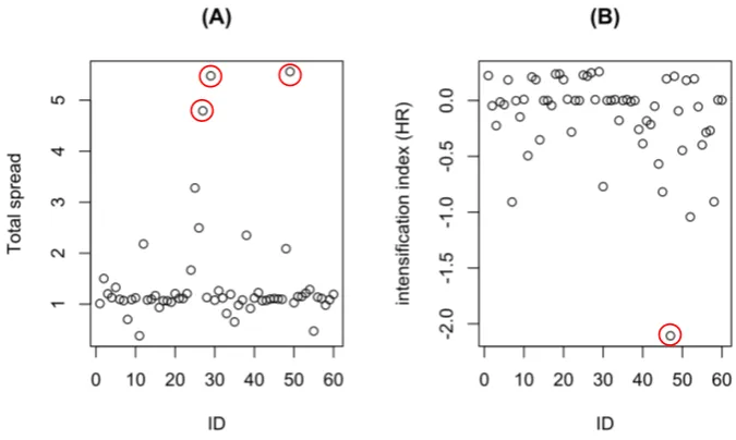
1.6.3 Outlier detection analysis
intensification index, seem to be appropriate statistics to detect eventual anomalies in the spatial and temporal components of the rating process as measured by computer-mouse movements and relative response time, respectively.
Data analysis and results. For the sake of simplicity, here we illustrate the outlier detection procedure using only the data associated to the fifth item of the reckless questionnaire described in the former application. We recall that this item described a situation where an individual drives under the influence of alcohol (see Table 1.2).
0 10 20 30 40 50 60
1
2
3
4
5
(A)
ID
Total spread
0 10 20 30 40 50 60
-2.0
-1.5
-1.0
-0
.5
0.
0
(B)
ID
intensification index (H
R)
FIGURE1.10: Example 3: Scatter plots for total spread and intensification index for outlier detection. Note that, red circles indicate outliers.
-400 -200 0 200 400
-400
-200
0
200
400
(A) Subj. 27
x
y
1 2
3
4 5
-400 -200 0 200 400
-400
-200
0
200
400
(B) Subj. 48
x
y
1 2
3
4 5
FIGURE1.11: Example 3: Anomalous empirical patterns of mouse movements.
time relative to the response times variance for the group of raters. Finally, we remark that in some situations it can be useful to produce a scatter plot between the total spread statistic and the intensification index. This com-bined representation would be used to jointly detect eventual anomalies in the spatial and temporal components of the rating process.
1.7
Final remarks
temporal components of the rating process. Such components were com-puted by the streaming of x-y computer-mouse coordinates and the over-all response times, respectively. In order to provide a final model rep-resentation for the rating data, we integrated such information using a fuzzy modeling paradigm. In particular, the motor component was repre-sented by an appropriate fuzzy set whereas the temporal component was included by modifying the shape of the spatial fuzzy set. The final fuzzy representation included all the information available from the response process (i.e., the final response, the temporal and spatial information, the fuzziness of the response, etc). To better illustrate the DYFRAT features, we also described two real applications from decision making and risk assessment contexts. The results suggested how DYFRAT can measure important features of dynamic decision process. We further showed as DYFRAT could be used to perform an outlier detection analysis.
1.7.1 Limitations
representations (Chung and Schwartz, 1995). Finally, at a more method-ological level a better validation of the advantages of our proposal com-pared with other existing methods for fuzzy ratings (e.g., FCS and FRS) should be tested in future works.
1.7.2 Conclusions
In sum, unlike other fuzzy scales, DYFRAT allows to express the fuzzi-ness of the human rating process by integrating two important physical measures. In this respect, DYFRAT always guarantees an ecological set-ting for cognitive measurements (e.g., it does not ask respondents to learn what fuzziness is and it works to express judgements/evaluations fuzzi-ness). Moreover, DYFRAT allows to model fuzziness as a natural prop-erty which spontaneously arises from some biometric measures (mouse-movements and response times) while respondents use a simple and user-friendly computer device to express their evaluations.
Representing the dynamics of rating
responses: An activation function
approach
An extended version of the chapter has been submitted as a research article toFrontiers in Psychology.
2.1
Introduction
Rating scales are probably the most commonly used measurement tools adopted in education, psychology, social science, and health research be-cause they are flexible scaling procedures for measuring attitudes, opin-ions, and subjective preferences (Göb, McCollin, and Ramalhoto, 2007; Miller and Salkind, 2002; Aiken, 1996; Pettit, 2002). A rating scale typi-cally consists of a variable to be measured and a set of anchor points from which the rater selects the most appropriate description. Among the rat-ing scales, the Likert-type scales are the most widely used scalrat-ing methods in education and social science. The main assumption for a Likert-scale is that the strength/intensity of the evaluation is linear, i.e. on a continuum from strongly agree to strongly disagree, with the neutral point being nei-ther agree nor disagree.
Although rating scales are generally as reliable and valid as more com-plex types of scaling methods (Nunnally, 1978), over the years several criticisms have been arisen against some well-known limitations with this
simple measurement approach. For example, because of the discrete and crisp nature of their format, some individuals tend to avoid extreme cat-egories in the scale (central tendency or restriction range problem) while selecting the final response (Domino and Domino, 2006). Moreover, in some empirical situations (i.e., personality inventories and attitude ) the honesty assumption, tacitly accepted in the administration of self-report rating scale, appears to be simply unrealistic and, therefore the measure-ments may result in biased observations (e.g., Furnham, 1986). Finally, the standard rating scale paradigm often regards human rating as a discrete-stage based process in which the final response represents its final discrete-stage only. Unfortunately, the observed final response simply captures the out-come of the rating process while the real-time cognitive dynamics that oc-cur during this process are usually lost. In particular, the standard observ-able measures generated during a rating task, the final discrete response and its associated response time, are simply end products of the underly-ing process of ratunderly-ing, not online measurements of it. In other words, they are indicators of the raters’ overall performance, but what really happens during a rating trial is clearly beyond their scope. However, understand-ing how mental representations unfold in time durunderstand-ing the performance of a rating task could be of relevant interest for many researchers work-ing in different empirical domains. Moreover, parswork-ing a ratwork-ing task into a sequence of subcomponents can help in constructing more sensible in-dices to detect effects which would otherwise be missed using the stan-dard overall performance measures.
2012; Magnuson, 2005; Freeman, Dale, and Farmer, 2011; Jansen, Black-well, and Marriott, 2003; Hwang et al., 2005; Chen, Anderson, and Sohn, 2001; Mueller and Lockerd, 2001; Freeman and Ambady, 2010; O’Reilly and Plamondon, 2011).
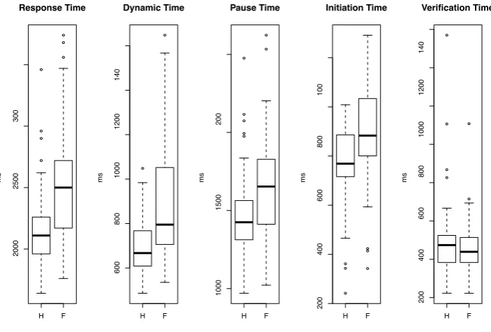
The new measures are assumed to be observable indicators of the dynamic process of rating which constitute the antecedents of the final rating out-come and they will allow a) to decompose the observed total rating time into a sequence of temporal subcomponents such as, for example, initi-ation time, pause time, verificiniti-ation time, and submovement time b) to represent the final response in terms of an activation value which mea-sures the level of intensity/strength for that response. Finally, in our approach both the components are integrated into a common functional model which allows to express the combined temporal and intensity lev-els of rating.
The remainder of this chapter is organized as follows. In the second sec-tion we present the overall idea underlying our approach and provide motivations to use it in human rating problems. In the third section we present our new methodology. In the fourth section we show two empiri-cal applications to real data, whereas in the fifth section we conclude this chapter by providing some final comments.
2.2
Rating evaluations as dynamic activation processes
to the center of the screen. The rater is asked to provide a response by mouse-clicking the chosen level of the scale (the selected anchor point). Meanwhile, the streaming of the x-y coordinates of the computer mouse (at a given sampling rate) as well as the time sequence of the movements are recorded and stored in the computer memory. The main idea of the dynamic rating framework is to represent each anchor point in the rat-ing scale by a dynamic activation state, which indicates (at each recorded time) the level of activation of that anchor point for the current mouse po-sition in the movement path. In general a level of activation at a given instant in time can be understood as a measure of the intensity/strength for the potential final response. The underlying assumption is as follows: the more the mouse pointer approaches the position of a selected anchor point in the pseudo-circular scale, the more the state of the corresponding rating response will be activated. This framework entails a competing ac-tivation system where each anchor point competes with the others for the final response. When the mouse pointer is located at the starting position (center of the screen), all the K distinct anchor points will be equally acti-vated at a certain baseline level. However, once the rater starts to use the mouse pointer and moves it in the two-dimensional space of the pseudo-circular scale, the anchor points with a shorter (Euclidean) distance from the current mouse position will start to show larger activation values. By contrast, the anchor points with a larger distance from the current mouse position will decrease their activation states. The proposed framework aims to represent for each potential final response its dynamic activation as a function of the temporal pattern of movements and the distance from the target anchor point position. Figure 2.1 shows a general diagram of mouse-movements with the associated activation functions.
2.2.1 Temporal and activation state measures
time (ms)
activation
valu
e
2 3
(A) (B)
FIGURE2.1: Hypothetical movement path with activation distributions and corre-sponding components of positioning time movements. Final response: anchor point 2.
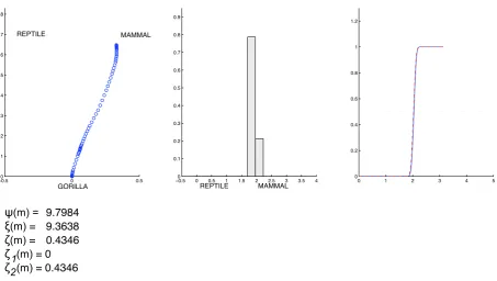
shown in 2.1. In particular, it shows a pattern of movements in which the spatio-temporal uncertainty is related to the rater’s choice between two possible alternatives. Note that the associated activation function for the final response has a more irregular shape characterized by two main peaks and one valley indicating the maximal activations for the options 3 and 2 and the change of direction from 3 to 2, respectively.
usually correspond to fast movement executions. Finally, the third feature describes the negative components, that is to say, the portions of the func-tion that are characterized by a negative slope (decreasing funcfunc-tion, see
β < 0 in Figure 2.2-B). Negative components denote active movements in the opposite direction of the final selected target. These usually reflect temporary deviations from the final response and are also characterized by fast movement executions. In particular, we assume that for execut-ing such submovements further information is taken into account by the rater (e.g., goal reformulation) and that in some circumstances
feedfor-ward information may be processed onthe fly during the same movement
production.
1
2
3
4 5
time (ms)
ac
tiv
ati
on
v
al
ue
β = 0
β = 0
β = 0
β = 0
β > 0 β >
0 β <
0
FIGURE2.2: Hypothetical movement path, activation distributions and correspond-ing dynamic components.
It is important to note that we can consider each of these functional fea-tures as events that are associated with a specific value of the time argu-ment of the function (see Figure 2.3). That is to say, the three features are characterized also by a temporal location.
time (ms)
activation
valu
e
time (ms)
activation
valu
e
FIGURE2.3: Quantitative time indices for summarizing the dynamics of the rating process: response time decomposition.
takes to check the location of the cursor and release the mouse button af-ter the last movement has ended. Finally, the positive components (resp. negative components) are associated withpositive submovement times(resp. negative submovement times) in the rating process. These subcomponents al-low us to additively decompose thetotal timeof the rating process into dif-ferent parts, each part denoting a difdif-ferent duration for a specific process involved in the dynamic rating behavior. The following decomposition rule for the response time (RT) holds:
RT = IT+IPT+ VT
| {z }
pause time
+ DT++DT−
| {z }
dynamic time
(2.1)
where:
• IT is the initiation time(from scale onset to first movement)
• IPT is the intermediate pause time
• VT is theverification time (from last movement to final clicking)
• DT+ is thepositive dynamic time (time spent toward the target)
• DT− is thenegative dynamic time (time spent away from the target)
of uncertainty in the rating process. Moreover, a high number of sub-movements (positive or negative) may reflect selection or choice related difficulties for the final rating response option.
In a similar way, we can also decompose the area under the dynamic acti-vation function into subareas according to the temporal phases described earlier (see 2.4).
time (ms)
activation
valu
e
time (ms)
activation
valu
e
FIGURE2.4: Quantitative time indices for summarizing the dynamics of the rating process: total activation decomposition.
In general, the area under the activation function indicates the level of in-tensity or strength for the final selected response. However, like for the times, also for the activation values the different subareas represent sepa-rate aspects of the rating process. So, for example, to measure the overall strength for the final response we must consider the sum of the activa-tion integrals associated with the positive submovements and eventually the time spent near the location of the final response (e.g., verification time). By contrast, the subareas associated with the negative submove-ments should indicate the amount of residual processes linked to tempo-rary deviations from the final response. The total activation (TA) decom-position is as follows:
TA = IA+ISA+ VA
| {z }
static activation
+ DA++DA−
| {z }
dynamic activation
(2.2)
• IA is theinitiation activation
• ISA is the intermediate static activation
• VA is theverification activation
• DA+is thepositive dynamic activation
• DA−is thenegative dynamic activation
Note that quantitative time indices and quantitative activation indices span different information for the rating process. So, for example, we may have two distinct movement pauses (e.g., initiation time and verification time) both characterized by the same interval length but with different overall activation values.
In sum, by using this simple functional framework, we can derive a num-ber of quantitative indices to provide predictions concerning various as-pects of the processes involved in the decision mechanism of a rating be-havior.
2.3
Methodology
Our proposal consists of a data-capturing procedure which implements a MTM based computerized interface for collecting the motor and temporal components in the process of rating and a data-modeling procedure which provides a functional model for the recorded information. Note that the interface for the data-capturing has been extensively described in the Chap-ter 1 (sections 1.4.1 and 1.5).
2.3.1 Data representation
Spatio-temporal data
Let p = (x,y) be the movement path with length H + 1 associated to the streaming of x-y Cartesian coordinates of the computer mouse movements
of recorded movements1). We assume that in p the first position p0 = (x0, y0)corresponds to the origin (0,0)(called starting position) of the
two-dimensional Cartesian plane R2, whereas ph = (xh, yh) denotes the hth el-ement (with h = 1, . . . , H) in the sequence of positions recorded in p. In particular, pH = (xH, yH) represents the final position in the path and usu-ally corresponds to the position in the two-dimensional plane of the final selected anchor point. Moreover, each position ph in the path is also as-sociated to a positive integer value th ∈ N denoting the time passed from the onset time of the pseudo-circular scale on the screen and the hth move-ment recorded in p. By definition we set t0 = 0 (initial time). Finally, the
total response time (or final time) t∗ is defined as the difference between the time at the mouse-clicking on the selected anchor point (final response) and the onset time of the pseudo-circular scale on the screen. In sum, the spatio-temporal sequence ((p0, t0),(p1, t1), . . . ,(pH, tH)) constitutes the en-tire information collected during a single rating trial and the array (p,t)is the correspondingspatio-temporal data structure.
From spatio-temporal data to functional data
The main assumption of our approach is to represent each anchor point in the rating scale by an activation state, which indicates (at each recorded time th) the level of activation of that anchor point for the current mouse positionphin the movement path. To model the activations we used a de-scriptive perspective based on the simple analogy with bivariate normal densities. In this context, the bivariate normal densities act as sensors to detect mouse movement positions. In particular, letfk(·|µk,Σ)be a
bivari-ate normal density with µk and Σ denoting the location parameter and
the scale parameter of the distribution, respectively. The location param-eter µk indicates the position in R2 of the kth anchor point in the pseudo-circular scale, whereas Σ is a diagonal covariance matrix with a single
parameter σ1 = σ2 = σ (the parameter sigma is called the anchor point
sensitivity). Each spatio-temporal observation (ph, th) in the movements path is associated to a positive real value akh ∈ R+ denoting the activation
of the kth anchor point (with k = 1, . . . , K) for the position ph recorded at time th. More precisely, the activation value is given by the following equation:
akh = fk(ph|µk, σ), h = 0, . . . , H; k = 1, . . . , K. (2.3)
Finally, the sequence(t,ak) = ((t0, ak0),(t1, ak1), . . . ,(tH, akH))is theactivation
data structure for the kth anchor point derived from the original spatio-temporal data (p,t). The basic idea is to think of the observed activation data as a single function instead of a simple sequence of individual obser-vations. Consequently, the activation data can be understood as functional data. More precisely, the term functional refers to the intrinsic structure of the data rather than to their explicit form (Ramsay and Silverman, 2005). Note that the activation functions are characterized by the following fea-tures: (a) because of the bivariate normal representation, the activation value is nonlinearly related with the distance between the current mouse position and the target anchor point position in the scale (b) the activation functions share all the same sensitivity valueσ(c) the distance from an an-chor point positionµkand the starting position(0,0)is held constant for all theK anchor points in the scale (d) the distance between two consecutive anchor point positions,µk andµk+1 (k = 1, . . . , K−1)is also held constant.
2.3.2 Data modeling and parsing
In our approach we assume that the curve being estimated is continuous and smooth. There are several methods that can be considered for ap-proximating discrete data by a function (for a review see Ramsay, 2006). In this contribution we adopted the roughness penalty or regularization ap-proach which is a powerful and flexible option for modeling functional data based on cubic B-spline basis functions (for more details the reader may refer to Ramsay and Silverman, 2002). Figure 2.5 shows the approxi-mation of the observed movement data represented in the panel A with a smooth activation function (panel B).
time
ac
tiv
ati
on
v
al
ue
(A) (B)
FIGURE2.5: Hypothetical movement path (A) with the associated smooth activation function (B).
One of the main advantages of modeling discrete data by a functional data analysis approach is that we can easily derive smooth approximations of the original activation data which may instead be characterized by not so regular representations due to the limitations of the empirical sampling rate.
parsing algorithm adapted from previous analytical techniques to detect corrective submovements. Our approach entails a systematic evaluation of the first derivative (velocity) of the activation function. In this evalua-tion, submovements as well as pauses are defined on the basis of certain criterion events (e.g., crossing of well-defined velocity thresholds). These criteria are chosen to take account of differences between the dynamics of voluntary movements (Meyer et al., 1988), physiological tremors and passive residual activity due to springlike characteristics of muscles. In particular, a static component of the activation function representing a movement pause was defined to be a continuous portion of the function such that the absolute value of its first derivative did not exceeded a given small positive threshold δ and the duration of the corresponding pause exceeded 20 ms.
time
ac
tva
to
n
va
ue
= 0
= 0
= 0
> 0 < 0
I order
derivativ
e
time
(A) (B)
FIGURE 2.6: Hypothetical smooth activation function (A) with the corresponding first-order derivative function (B). Note that dotted lines refers to a parsing grid.
The latter means that a positive submovement (resp. negative submove-ment) must show activation values with positive first derivatives exceed-ingδ(resp. with negative first derivatives not exceeding−δ) and remained above (resp. below) that level continuously for at leas