Volume 28 - Article 18 | Pages 505–546

(1)

A peer-reviewed, open-access journal of population sciences

DEMOGRAPHIC RESEARCH

VOLUME 28, ARTICLE 18, PAGES 505-546

PUBLISHED 15 MARCH 2013

http://www.demographic-research.org/Volumes/Vol28/18/ DOI: 10.4054/DemRes.2013.28.18

Research Article

Estimating global migration flow tables using

place of birth data

Guy J. Abel

c

2013 Guy J. Abel.

(2)

2 Methodology 508

2.1 Extensions for non-movers 514

2.2 Extensions to include births, deaths, and flows to and from outside regions 519

3 Results 525

3.1 Application 525

3.2 Summary of estimates 526

4 Validation of results 534

4.1 Net migration comparison 534

4.2 Gravity model 537

5 Summary and discussion 540

6 Acknowledgements 542

(3)

Estimating global migration flow tables using place of birth data

Guy J. Abel1

Abstract

BACKGROUND

International migration flow data often lack adequate measurements of volume, direction and completeness. These pitfalls limit empirical comparative studies of migration and cross national population projections to use net migration measures or inadequate data.

OBJECTIVE

This paper aims to address these issues at a global level, presenting estimates of bilateral flow tables between 191 countries.

METHODS

A methodology to estimate flow tables of migration transitions for the globe is illustrated in two parts. First, a methodology to derive flows from sequential stock tables is devel-oped. Second, the methodology is applied to recently released World Bank migration stock tables between 1960 and 2000 (Özden et al. 2011) to estimate a set of four decadal global migration flow tables.

RESULTS

The results of the applied methodology are discussed with reference to comparable esti-mates of global net migration flows of the United Nations and models for international migration flows.

COMMENTS

The proposed methodology adds to the limited existing literature on linking migration flows to stocks. The estimated flow tables represent a first-of-a-kind set of comparable global origin destination flow data.

1_{Wittgenstein Centre (IIASA, VID/ÖAW, WU), Vienna Institute of Demography/Austrian Academy of}

(4)

1. Introduction

International moves are typically enumerated in a demographic context using either a measurement of migrant stocks or migration flows. A migrant stock is defined as the total number of international migrants present in a given country at a particular point of time. A migration flow is defined as the number of persons arriving or leaving a given country over the course of a specific period of time. Flow measures reflect the dynamics of the migration process and are typically considered to be less tractable than stock measures (Bilsborrow et al. 1997, p.51).

International migration flow data often lacks adequate measurements of volume, di-rection and completeness (Kelly 1987; Salt 1993; Willekens 1994; Nowok, Kupiszewska, and Poulain 2006), making cross national comparisons difficult. The lack of compa-rability in flow data can be traced to a number of causes. First, migration is a multi-dimensional process (Goldstein 1976) involving a transition between two states. Con-sequently, movements can be reported by sending or receiving countries. When data collection methods or measurements in countries differ, the reported counts do not match. Second, international migration flow data are typically collected by individual national statistics institutes in each country, where measures have been designed to suit solely do-mestic priorities. Data are often produced within a legal framework, and hence alterations to their collection are difficult to implement. Finally, in many countries data collection systems for migration flow data do not exist. In other countries, collection methods such as passenger surveys may prove inadequate to report flows at the levels of detail required by some data users.

(5)

as illustrated in the methodological section of this paper, can be used as a basis to estimate global bilateral migration flow tables.

Estimates of global bilateral flow tables can potentially have a number of advantages over presently available international migration data. First, they allow a fuller understand-ing of population behaviour and change in comparison to other measures of migration. Studying people’s movements using both origin and destination dimensions furthers the possibility of deeper insights into migration patterns and migrant behaviours. Such in-sights can be confounded by more conventional methods of analysis on existing measures of migration flows, such as those to or from only a few select nations, or through the study of net migration. Second, bilateral migration flow tables allow a comparison of mi-gration propensities across multiple countries. Consequently, the contributions made by each nation to the global system of migration can be more easily identified, and compar-ative summaries of migration flows become more meaningful in a multinational context. Third, estimates of bilateral migration flow tables permit a more comprehensive empiri-cal source for testing migration theories. In addition, the study of public policies towards the control or encouragement of migration flows can be further expanded to incorporate a wider evidence base. Fourth, while stock data can be collected more easily than flow data, information on migration patterns from studying stocks can potentially provide a poor in-dication of contemporary international migration flows. Furthermore, in countries where there are significant return migrations or mortality among foreign population, migrant stock data can a yield a misleading portrait of the current migration system (Massey et al. 1999, p.200). Fifth, estimates of international migration flow tables can provide a more perceptive base data for global population forecasts. Current global population forecasts, such as KC et al. (2010) or United Nations Population Division (2011) utilise only esti-mated international net migration totals, where no other comparable migration data exists for population forecasters on such scales (Kupiszewski and Kupiszewska 2008). As such, global forecasting exercises often run the risk of well documented problems of using net migration measures in their models; see for example Rogers (1990) or Rogers (1995). These potential benefits are leading international organisations to call for the promotion and development of methodologies for the collection and processing of internationally comparable statistical data on international migration (United Nations General Assembly 2011).

(6)

mi-gration flows. The second and third papers rely on detailed disaggregation of stock data, which are not currently available for international migration data at the global scale.

In this paper a new methodology to estimate global flow tables of migrant transitions between all countries is illustrated in two parts. First, a methodology to derive flows from sequential stock tables is developed. Using a set of simple hypothetical data, rather than a full global table, the methodology is initially demonstrated in a scenario where there are no births and deaths in migrant stock populations between two periods. An extension for natural changes in population totals is then shown. Estimation is undertaken using a spa-tial interaction model, equivalent to a log-linear model in statistics. Such methods have a developed literature in the indirect estimation of internal migration flows, where marginal totals (immigration and emigration flows into and out of a set of regions) are known, but the table contents are missing, see for example Fotheringham and O’Kelly (1988) or Willekens (1999). Second, the methodology is applied to recently released World Bank migration stock tables between 1960 and 2000 (Özden et al. 2011) to estimate a set of four decadal global migration flow tables. Summary results of the applied methodology are first presented and then discussed with reference to comparable estimates of global net migration flows of the United Nations and models for international migration. These validation exercises give an indication of the performance of the applied methodology. In the final section, potential extensions are outlined and conclusions given.

2. Methodology

A general methodology for the estimation of migration flows from sequential migrant stock tables is derived in this section. The estimation of migration flows between a set of regions is illustrated using a set of simple hypothetical data. Increasing complexity is added to account for additional factors that might also effect changes in stock totals, be-sides migration flows, such as births, deaths, and movements to and from external regions not considered.

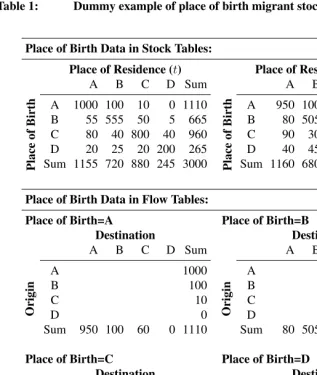
Bilateral migration data are commonly represented in square tables. Values within the table vary, depending on definitions used in data collection or the research question at hand. Values in non-diagonal cells represent some form of movement, for example a migration flow between a specified set ofR regions or areas or a foreign born stock. Values in diagonal cells represent some form of non-moving population, or those that move within a region, and are sometimes not presented.

(7)

Table 1: Dummy example of place of birth migrant stock data

Place of Birth Data in Stock Tables:

Place of Residence (t) Place of Residence (t+ 1)

A B C D Sum A B C D Sum

Place

of

Birth

A 1000 100 10 0 1110

Place

of

Birth

A 950 100 60 0 1110

B 55 555 50 5 665 B 80 505 75 5 665

C 80 40 800 40 960 C 90 30 800 40 960

D 20 25 20 200 265 D 40 45 0 180 265

Sum 1155 720 880 245 3000 Sum 1160 680 935 225 3000

Place of Birth Data in Flow Tables:

Place of Birth=A Place of Birth=B

Destination Destination

Origin

A 1000

Origin

A 55

B 100 B 555

C 10 C 50

D 0 D 5

Sum 950 100 60 0 1110 Sum 80 505 75 5 665

Place of Birth=C Place of Birth=D

Origin

A 80

Origin

A 20

B 40 B 25

C 800 C 20

D 40 D 200

Sum 90 30 800 40 960 Sum 40 45 0 180 265

(8)

individuals change their place of residence (moving across columns), while their place of birth (row) characteristic remains fixed.

To derive a corresponding set of flows that are constrained to meet the stocks tables, we can alternatively consider the top panel of Table 1 as a set ofR birthplace specific migration flow tables where the marginal totals are known, shown in the bottom panel of Table 1. These are formed by considering each row of the two consecutive stock tables as a set of separate margins of a migration flow table. Place of residence totals at timet

from the stock data now become origin margin (row) totals for each birth place specific population. Similarly, place of residence totals at timet+ 1from the stock data now become destination margin (column) totals for each birth place specific population. As the row totals from the stock tables are equal, the row and column margins in each of the birth place specific migration flow tables in Table 1 are also equal.

Typically migration flow measures can be classified as movement or transition data (Rees and Willekens 1986). Movement data consist of counts migration events across boundaries. Transition data consist of counts of migrants whose location at the end of a specified time periods is different to that at the beginning of the period. Within each birthplace specific table in the bottom panel of Table 1, missing non-diagonal cells must represent the migrant transition flows from originito destinationj, within time periodt

tot+ 1and categorised by birthplacek. Missing diagonal entries represent the number of people who reside in the same region attandt+ 1, which are referred to as stayers throughout the remainder of this paper. In order to estimate the missing migrant transition flows and stayers, model based methods are used to impute values that are constrained to the known marginal totals.

Flowerdew (1991) outlined two main approaches for the use of models to either anal-yse or estimate flow tables for internal migration data: the gravity model and the spatial interaction model. The gravity model approach derives from movements between re-gions in a similar manner to particle responses to two gravitational masses, as proposed by Newton in Principia Mathematica. Stewart (1941) and Zipf (1942) framed this ap-proach for migration data, relying on statistical estimation of migration volumes, given information on each origin, destination and a measurement of association between them. The spatial interaction models, associated with Wilson (1970), are based on mathematical algorithms to calibrate a constrained model to origin and destination totals. There are numerous formulations of spatial interaction models such as bi-proportional adjustment, information gain minimizing and entropy maximizing which include various constraints and interaction terms (Willekens 1983).

(9)

destina-tion constrained spatial interacdestina-tion model, and when both covariates are present, a doubly constrained spatial interaction is obtained. Such representations, with only categorical covariates, are equivalent to the log-linear regression models of Birch (1963). When row or column dummy covariates are not included, but other origin and destination specific factors are, such as population size, the resulting Poisson regression model is equivalent to the gravity model first proposed by Zipf (Flowerdew 1991).

A simplistic version of the spatial interaction model for the number of migrants in transition nij from origin ito destination j, during the respective time interval, as in

each of theR = 4incomplete data situations of the bottom panel of Table 1, may be considered;

yij=αiβjmij (1)

whereyij is the expected number of migrants in transition from originito destinationj

andi, j= 1,2, . . . , RforRorigins and destinations. Theαiandβjparameters represent

the background factors that are related to the characteristics of the origin and destination. Themijfactor represents some auxiliary information on migration flows. This is typically

additional data related to migration between the same origins and destinations. Willekens (1999) noted, in conventional spatial interaction analysis,mij = F(dij)wheredij is a

measure of distance betweeniandj andF(.)is a distance deterrence function. Such distance deterrence functions can come in different forms, such as F(dij) = d−ij or

F(dij) = exp(−dij), where >0is a distance sensitivity parameter; see Sen and Smith

(1995, p4). Alternative specifications formij might be travel costs or past migration

flows.

As described by Willekens (1999), the estimation of parameters in a spatial interaction model can be performed by re-expressing the spatial interaction model of (1) in terms of a log-linear model:

logyij = logαi+ logβj+ logmij, (2)

where unlike standard log-linear models, no intercept is included, and the final term is commonly referred to as an offset. The maximum likelihood estimates for theαiandβj

parameters in (2) can be derived by considering the probability of observingnijmigrant

transitions during a unit interval, given by the Poisson distribution function:

P(Nij =nij) =

ynij

ij

nij!

exp(−yij). (3)

The likelihood function forY={yij, i, j,= 1, . . . , R}givenn={nij, i, j,= 1, . . . , R}

migrant transitions, provided that migrant transitions are independent, is

L(Y;n) =P(N11=n11, N12=n12, . . . , NRR=nRR) =

Y

ij

ynij

ij

nij!

(10)

Inserting the log-linear spatial model of (1) into expression (4) and taking the logarithmic transformation gives the log-likelihood function:

l(θ;n) =X

ij

{nijlog(αiβjmij)−αiβjmij−log(nij!)}

=X

i

ni+log(αi) +

X

j

n+jlog(βj)−

X

ij

αiβjmij+c,

(5)

whereθ ={αi, βj, i, j= 1, . . . , R},ni+ =P

j

nij andn+j =P i

nij are the marginal

totals, and

c=X

ij

nijlog(mij)−

X

ij

log(nij!). (6)

The maximum likelihood estimates ofαi andβj are obtained by maximising the

log-likelihood function (5). The extra termc, which does not involve the parameters, may be ignored. Thus, conveniently only the marginal totals from the consecutive stock tables are required to estimate the spatial interaction model.

Differentiation of the likelihood function with respect to each parameter gives us the likelihood equations:

∂l ∂αi

=ni+ αi

−X

j

βjmij = 0 (7)

and

∂l ∂βj

= n+j βj

−X

i

αimij = 0. (8)

The maximum likelihood estimators forαiandβj can then be written as

ˆ αi=

ni+ P

j

ˆ βjmij

(9)

and

ˆ βj =

n+j

P

i

ˆ αimij

. (10)

Direct estimates ofαiandβjcannot be obtained, since there are no closed-form

(11)

ˆ

β(0)_j , estimates of αˆ(1)_i = ni+ .

P

j

ˆ

β(0)_j mij. These estimates are then used to update

ˆ

β(2)_j =n+j

. P

i

ˆ

α(1)_j mij. This process repeats until convergence. Maximum likelihood

estimates ofyij, the expected number of migrant transitions, are deduced from the

con-verged estimates ofαˆiandβˆjusing the spatial interaction model of (1). Willekens (1999)

discusses how this procedure is a special case of the iterative proportional fitting algo-rithm and the Expectation-Maximisation (EM) algoalgo-rithm. As noted in Raymer, Abel, and Smith (2007), this is also a conditional maximisation, also known as a stepwise ascent.

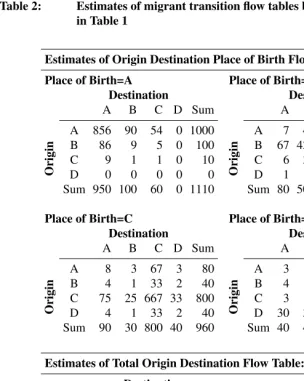
Using the sufficient statistics ofnshown in Table 1 and the converged estimates of

ˆ

αiandβˆj in the spatial interaction model (12) gives the maximum likelihood estimates

of yij, the expected number of migrant transitions. These values are shown in the top

panel of Table 2 for each birthplace specific table. The iterative procedure to estimate

ˆ

αiandβˆj andyij is undertaken using thecm2routine in themigestR package (Abel

2012), where all elements ofmijare set to unity (mij = 1). Summing over all birthplaces

and deleting stayers in the diagonal elements results in a traditional flow table of migrant transitions from originito destinationjduring the time periodttot+ 1shown in the bottom panel of Table 2.

The spatial interaction model of (1) focuses on estimating migrant transitions between two dimensions, origin and destination (rows and columns). This model can be assumed to derive estimates in each of the individualR = 4birthplace specific flow tables pre-sented in the bottom panel of Table 1. Alternatively, the model can be expanded to include a third (table) dimension by adding parameters to consider all birthplace specific tables simultaneously,

logyijk= logαi+ logβj+ logλk+ logγik+ logκjk+ logmij (11)

whereyijkis the expected number of migrant transitions from originito destinationjof

people born in birthplacek, during the respective time interval andi, j, k = 1,2, . . . , R, forRorigins, destinations and birthplaces. Theαi,βjandλkparameters represent

back-ground factors that relate to the characteristics of the origins, destinations and birthplaces respectively. Theγikandκjkparameter sets represent the factors specific to each

(12)

Table 2: Estimates of migrant transition flow tables based on stock data in Table 1

Estimates of Origin Destination Place of Birth Flow Tables:

Origin

A 856 90 54 0 1000

Origin

A 7 42 6 0 55

B 86 9 5 0 100 B 67 421 63 4 555

C 9 1 1 0 10 C 6 38 6 0 50

D 0 0 0 0 0 D 1 4 1 0 5

Sum 950 100 60 0 1110 Sum 80 505 75 5 665

Origin

A 8 3 67 3 80

Origin

A 3 3 0 14 20

B 4 1 33 2 40 B 4 4 0 17 25

C 75 25 667 33 800 C 3 3 0 14 20

D 4 1 33 2 40 D 30 34 0 136 20

Sum 90 30 800 40 960 Sum 40 45 0 180 265

Estimates of Total Origin Destination Flow Table: Destination

A B C D Sum

Origin

A 138 127 17 282

B 160 101 23 284

C 93 67 47 207

D 35 39 34 107

Sum 287 244 262 87 881

2.1 Extensions for non-movers

(13)

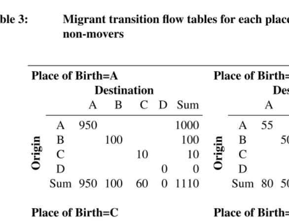
Abel, and Smith (2007). However, the margins under consideration have traditionally been sums of inflows and outflows, to and from, a set of regions. The marginal data in the bottom panel of Table 1 is based on a combination of migrant transitions and stayers. Hence, in order to estimate solely the migrant transitions, an assumption about the number of stayers in the migration system must be taken, and a model adapted accordingly. Not extending a model to account for differences in migrants and stayers would effectively impose the assumption that the cost of migration is the same as the cost not to migrate. One such extension is to fix the diagonal terms in each sub-table to their maximum value, without violating each corresponding marginal constraints, as in Table 3.

Table 3: Migrant transition flow tables for each place of birth with assumed non-movers

Origin

A 950 1000

Origin

A 55 55

B 100 100 B 505 555

C 10 10 C 50 50

D 0 0 D 5 5

Sum 950 100 60 0 1110 Sum 80 505 75 5 665

Origin

A 80 80

Origin

A 20 20

B 30 40 B 25 25

C 800 800 C 0 20

D 40 40 D 180 200

Sum 90 30 800 40 960 Sum 40 45 0 180 265

Consequently, the non-diagonal estimates will represent the minimum number of mi-gration transitions from originito destinationjbetween timetandt+1while maintaining marginal constraints.

(14)

addi-tional parameter can be added to (11),

logyijk= logαi+logβj+logλk+logγik+logκjk+logδijkI(i=j)+logmij, (12)

whereI(·)is the indicator function,

I(i=j) =

(

1 ifi=j 0 ifi6=j ,

and the correspondingδijk parameter set represents the factors specific to each set of

stayers.

The log-likelihood function corresponding to the spatial interaction model in (12), where, for simplicity,δijkis now referred to asδiik, is

l(θ;n) =X

ijk

{nijklog(αiβjλkγikκjkδiikmij)−αiβjλkγikκjkδiikmij−log(nijk!)}

=X

i

ni++log(αi) +

X

j

n+j+log(βj) +

X

k

n++klog(λj)

+X

ik

ni+klog(γik) +

X

jk

n+jklog(κjk) +

X

ijk

nijklog(δiik)

−X

ijk

αiβjλkγikκjkδiikmij+c, (13)

whereθ={αi, βj, λk, γik, κjk, δiik, i, j, k= 1, . . . , R},n={nijk, i, j, k= 1, . . . , R}

and

c=X

ijk

nijklog(mij)−

X

ijk

log(nijk!). (14)

(15)

likelihood equations:

∂l ∂αi

= ni++ αi

−X

jk

βjλkγikκjkδiikmij = 0,

∂l ∂βj

= n+j+ βj

−X

ik

αiλkγikκjkδiikmij = 0,

∂l ∂λk

= n++k λk

−X

ij

αiβjγikκjkδiikmij = 0,

∂l ∂γik

= ni+k γik

−X

j

αiβjλkκjkδiikmij = 0, (15)

∂l ∂κjk

= n+jk κjk

−X

i

αiβjλkγikδiikmij = 0,

∂l ∂δiik

= nijk δiik

−αiβjλkκjkγikmij = 0,

which require only the marginal totals displayed in Table 3, (ni++,n+j+,n++k,ni+k

andn+jk) and the diagonal values (nijk, wherei=j). The likelihood equations can be

used to derive maximum likelihood estimators forθˆ= ( ˆαi,βˆj,λˆk,ˆγik,ˆκjk,δˆiik);

ˆ αi=

ni++ P

jk

ˆ

βjλˆkγˆikκˆjkδˆiikmij

,

ˆ βj=

n+j+ P

ik

ˆ

αiˆλkˆγikκˆjkˆδiikmij

,

ˆ λk=

n++k

P

ij

ˆ

αiβˆjγˆikˆκjkδˆiikmij

,

ˆ γik=

ni+k

P

j

ˆ

αiβˆjλˆkˆκjkδˆiikmij

,

ˆ κjk=

n+jk

P

i

ˆ

αiβˆjλˆkˆγikδˆiikmij

,

ˆ δiik=

nijk

ˆ

αiβˆjλˆkγˆiikˆκjkmij

,

(16)

and can be solved by iteration using six steps for each parameter set:

ˆ

α_i(1)= ni++

P

jk

ˆ

β_j(0)ˆλ(0)_k ˆγ_ik(0)κˆ(0)_jkδˆ(0)_iikmij

,

ˆ

β_j(2)= n+j+

P

ik

ˆ

α(1)_i λˆ(0)_k γˆ_ik(0)ˆκ(0)_jkδˆ(0)_iikmij

,

ˆ

λ(3)_k = n++k

P

ij

ˆ

α(1)_i βˆ(2)_j ˆγ_ik(0)κˆ(0)_jkˆδ_iik(0)mij

,

ˆ

γ_ik(4)= ni+k

P

j

ˆ

α(1)_i βˆ(2)_j ˆλ_k(3)κˆ(0)_jkδˆ(0)_iikmij

,

ˆ

κ(5)_jk = n+jk

P

i

ˆ

α(1)_i βˆ(2)_j ˆλ_k(3)γˆ_ik(4)δˆ(0)_iikmij

,

ˆ

δ_iik(6)= nijk ˆ

α(1)_i βˆ_j(2)λˆ_k(3)γˆ_ik(4)ˆκ(5)_jkmij

.

(17)

Once one cycle of estimation is complete, a new cycle commences using the last set

of parameter estimates,αˆ(7)_i =ni++ .

P

jk

ˆ

β_j(2)λˆ(3)_k ˆγ(4)_ikκˆ(5)_jkδˆ(6)_iikmij, and so on. This is a

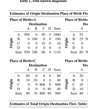
conditional maximization of the likelihood function and converges to give estimates of all the parameters inθ. Note that the choice of initial values ofβ(0)_j , λ(0)_k , γ_ik(0), κ(0)_jk, δ(0)_iikin each of (17) implicitly specifies the constraint that is required for parameter identification. Using the sufficient statistics ofnshown in Table 3 to obtain the converged estimates ofθˆin the spatial interaction model (12), the maximum likelihood estimates ofyijk, the

expected number of migrant transitions can be derived. These values are shown in the top panel of Table 4. The iterative procedure to estimateθˆandyijk is undertaken using

theipf3.qiroutine in themigestR package (Abel 2012), where all elements ofmij

are set to unity (mij = 1). Summing over all birthplaces and deleting stayers in the

diagonal elements gives us a traditional flow table of migrant transitions from origini

(17)

Table 4: Estimates of migrant transition flow tables based on stock data in Table 1, with known diagonals

Origin

A 950 0 50 0 1000

Origin

A 55 0 0 0 55

B 0 100 0 0 100 B 25 505 25 0 555

C 0 0 10 0 10 C 0 0 50 0 50

D 0 0 0 0 0 D 0 0 0 5 5

Sum 950 100 60 0 1110 Sum 80 505 75 5 665

Origin

A 80 0 0 0 80

Origin

A 20 0 0 0 20

B 10 30 0 0 40 B 0 25 0 0 25

C 0 0 800 0 800 C 10 10 0 0 20

D 0 0 0 40 40 D 10 10 0 180 200

Sum 90 30 800 40 960 Sum 40 45 0 180 265

A B C D Sum

Origin

A 0 50 0 50

B 35 25 0 60

C 10 10 0 20

D 10 10 0 20

Sum 55 20 75 0 150

2.2 Extensions to include births, deaths, and flows to and from outside regions

(18)

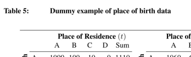
can move to or from regions outside those under consideration. We will consider each of these three sources of population change in this sub-section using a new set of hypo-thetical data fort+ 1, displayed in Table 5, where differences between row totals in the two stock tables now exist in comparison to the data in Table 1. In each case, popula-tion stocks that form the margins of the birthplace specific flow tables must be adjusted to enable the row and column margins to equal. This is carried out through a four step procedure.

Table 5: Dummy example of place of birth data

Place of Residence(t) Place of Residence(t+ 1)

Place

of

Birth

A 1000 100 10 0 1110

Place

of

Birth

A 1060 60 10 10 1140

B 55 555 50 5 665 B 45 540 40 0 625

C 80 40 800 40 960 C 70 75 770 70 985

D 20 25 20 200 265 D 30 30 20 230 310

Sum 1155 720 880 245 3000 Sum 1205 705 840 310 3060

(19)

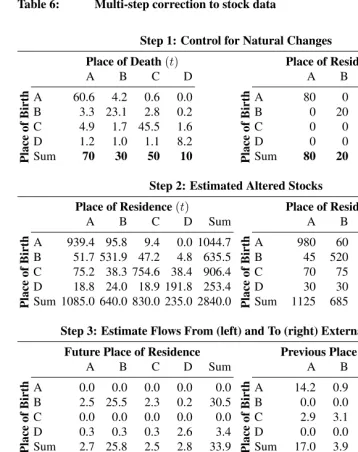
Table 6: Multi-step correction to stock data

Step 1: Control for Natural Changes

Place of Death(t) Place of Residence(t+ 1)

A B C D A B C D

Place

of

Birth

A 60.6 4.2 0.6 0.0

Place

of

Birth

A 80 0 0 0

B 3.3 23.1 2.8 0.2 B 0 20 0 0

C 4.9 1.7 45.5 1.6 C 0 0 40 0

D 1.2 1.0 1.1 8.2 D 0 0 0 60

Sum 70 30 50 10 Sum 80 20 40 60

Step 2: Estimated Altered Stocks

Place

of

Birth

A 939.4 95.8 9.4 0.0 1044.7

Place

of

Birth

A 980 60 10 10 1060

B 51.7 531.9 47.2 4.8 635.5 B 45 520 40 0 605

C 75.2 38.3 754.6 38.4 906.4 C 70 75 730 70 945

D 18.8 24.0 18.9 191.8 253.4 D 30 30 20 170 250

Sum 1085.0 640.0 830.0 235.0 2840.0 Sum 1125 685 800 250 2860

Step 3: Estimate Flows From (left) and To (right) External Regions Future Place of Residence Previous Place of Residence

Place

of

Birth

A 0.0 0.0 0.0 0.0 0.0

Place

of

Birth

A 14.2 0.9 0.1 0.0 15.3

B 2.5 25.5 2.3 0.2 30.5 B 0.0 0.0 0.0 0.0 0.0

C 0.0 0.0 0.0 0.0 0.0 C 2.9 3.1 29.8 2.9 38.6

D 0.3 0.3 0.3 2.6 3.4 D 0.0 0.0 0.0 0.0 0.0

Sum 2.7 25.8 2.5 2.8 33.9 Sum 17.0 3.9 30.0 3.0 53.9

Step 4: Re-estimated Altered Stocks

of

Birth

A 939.4 95.8 9.4 0.0 1044.7

of

Birth

(20)

In order to avoid estimating migration flows to meet increases in native born totals from newborns, the number of births betweentandt+ 1is subtracted from the reported stock data at timet+ 1. As with deaths, we tend to only have information on the total number of births, where ideally more detail on the place of residence of newborns at time

t+ 1is desired. In order to adjust stock totals for natural increases, births are assumed to only affect the native born stocks, assuming there is no migration of newborns. This is illustrated on the right hand side of Step 1 in Table 6, where the total number of births, given in bold type face in the final sum row, is known. These totals of newborns are allocated to reside in their place of birth at timet+ 1.

A new set of adjusted stock tables that account for natural population change are shown in Step 2 of Table 6, where both the death and birth estimates of the previous step are subtracted cell-wise from the original data in Table 5. The new altered stock tables still do not have equal row totals. If the estimates (and assumptions) about the changes to population stocks from natural causes are true, the remaining differences between the row totals in the altered stock tables must represent the minimum amount of migrant transitions to or from outside external regions beyond A to D. When this difference is greater than zero, i.e. the row totals for time periodt+ 1are greater thant, migrants have arrived from external regions. When this difference is less than zero, i.e. the row totals for time periodt+ 1are smaller thant, migrants have moved away to external regions. Adjustments can be made for these differences in order to estimate migration solely within regions under consideration (A to D).

To illustrate the estimation of migrant transition flows to and from external regions, consider Step 2 of Table 6 where the adjusted stock of people originally born in region A were1044.66and1060in timetandt+ 1respectively. Note, fractions of migrants are given only to fully illustrate the mathematics at work. As the difference is negative

(21)

A new set of altered stock totals that adjust for migration flows to and from external regions are shown in Step 4 of Table 6. These are calculated by subtracting cell-wise the previously adjusted stock totals in Step 2 from the calculated flows to other regions in Step 3. The resulting stock tables control for both natural population change and moves to and from external regions during the time periodt tot+ 1. In addition, they have matching row totals, required to estimate flows using the methodology outlined in the previous subsection.

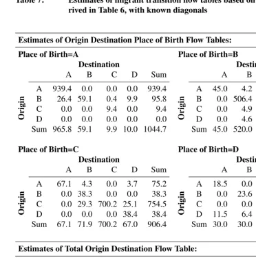
The sufficient statistics ofnshown in Stage 4 of Table 6 can be considered as a set ofR = 4birthplace specific flow tables, shown in the margins in the top panel of Table 7. Using these marginal data and the converged estimates ofθˆin the spatial interaction model (12) we obtain the maximum likelihood estimates ofyijk, the expected number

of migrant transitions, controlling for natural population changes and moves to and from external regions. These values are shown in the cells of the tables in the top panel of Table 7. The iterative procedure to estimateθˆandyijk, controlling for flows to and from outside

regions is undertaken using theffsroutine in themigestR package (Abel 2012). By default, in theffsroutine all elements ofmijare set to unity (mij = 1) and the diagonal

element are set to their maximum possible values given the known margins. Summing over all birthplaces and deleting stayers in the diagonal elements gives us a traditional flow table of migrant transitions from originito destinationjduring the time periodtto

(22)

Table 7: Estimates of migrant transition flow tables based on stock data de-rived in Table 6, with known diagonals

Origin

A 939.4 0.0 0.0 0.0 939.4

Origin

A 45.0 4.2 0.0 0.0 49.2

B 26.4 59.1 0.4 9.9 95.8 B 0.0 506.4 0.0 0.0 506.4

C 0.0 0.0 9.4 0.0 9.4 C 0.0 4.9 40.0 0.0 44.9

D 0.0 0.0 0.0 0.0 0.0 D 0.0 4.6 0.0 0.0 4.6

Sum 965.8 59.1 9.9 10.0 1044.7 Sum 45.0 520.0 40.0 0.0 605.0

Origin

A 67.1 4.3 0.0 3.7 75.2

Origin

A 18.5 0.0 0.0 0.0 19.0

B 0.0 38.3 0.0 0.0 38.3 B 0.0 23.6 0.0 0.0 23.6

C 0.0 29.3 700.2 25.1 754.5 C 0.0 0.0 18.6 0.0 18.6

D 0.0 0.0 0.0 38.4 38.4 D 11.5 6.4 1.4 170.0 189.2

Sum 67.1 71.9 700.2 67.0 906.4 Sum 30.0 30.0 20.0 170.0 250.0

A B C D Sum

Origin

A 8.5 0.0 3.7 12.2

B 26.4 0.4 9.9 36.7

C 0.0 34.2 25.1 59.3

D 11.5 10.9 1.4 23.8

(23)

3. Results

In this section the application of the above methodology to global place of birth migrant stock tables produced by the World Bank (Özden et al. 2011) is outlined, alongside the additional data requirements. A brief overview of the results, focusing on the largest estimated flows is discussed below.

3.1 Application

Place of birth data published by the World Bank (Özden et al. 2011) provide foreign born migration stock tables at the start of each of the last five decades for 226 countries2_{. To} date, this is the most complete set of comparable global data of past international migra-tion stocks available. The data are primarily based on place of birth responses to census questions or details collected from population registers. In order to create a complete and comparable data set, the World Bank undertook a number of adjustment and imputation steps. What follows is a brief description; for full details the reader is referred to Özden et al. (2011). For some nations, where there is no place of birth data available, data on citizenship are taken by the World Bank with the belief that they are a broadly equivalent measure of migrant stock populations. In other countries where neither place of birth or citizenship stock measure was available, missing values were addressed using various propensity and interpolation methods. These were either based on historical or future data when a measure in a specific period was missing, or using available data from countries in the same region when data in all periods were missing. Changes in geography, from countries unifying or partitioning were also accounted on a country by country basis using various imputation measures depending on available related data. For example, historical stocks by place of birth in former USSR countries were not collected in the 1960 to 1980 census rounds, however questions were asked on ethnicity. In the 1989 census both stocks by ethnicity and place of birth data were reported, allowing a proxy measure of past place of birth stocks to be derived.

Of the 226 countries for which stock data was available, 191 also had the demographic data from the United Nations Population Division (2011)3 throughout the time periods, as required for estimating flow methodology outlined in the previous section. None of the dropped countries had populations in in excess of 100,000 people 2010. Diagonal el-ements in the stock tables, of the native-born population totals in each place of residence

j, (PN B

j ), are not provided in the World Bank data. These were derived as a remainder

(PN B

j =Pj−P_iPjF B) using annual population totals from the United Nations

Popu-lation Division (2011), (Pj) and the column sums of the foreign born populations in each

(24)

place of residence (P

iP F B

j ). This procedure constrained the column totals of the stock

tables to meet those of the reported populations at the start of each decade.

Demographic data on the number of births and deaths in each country, required in the multi-step estimation shown in Table 6, were also taken from United Nations Popu-lation Division (2011). Auxiliary data for use in the offset term of the estimation proce-dure were taken from the Centre d’Etudes Prospective et d’Informations Internationales (CEPII) data base on geographic distance (Mayer and Zignago 2012), which provides a distance measure between all capital cities. The offset term was then calculated as

mij =d−ij1. The multi-step accounting method was undertaken to adjust reported stock

totals for births, deaths, and flows to external countries beyond the 191 considered. The conditional maximisation routine was then run to calculate the migration flow tables for each decade between the five sets of migration stock tables. Both of these process were undertaken within theffsroutine in themigestR package (Abel 2012).

3.2 Summary of estimates

(25)

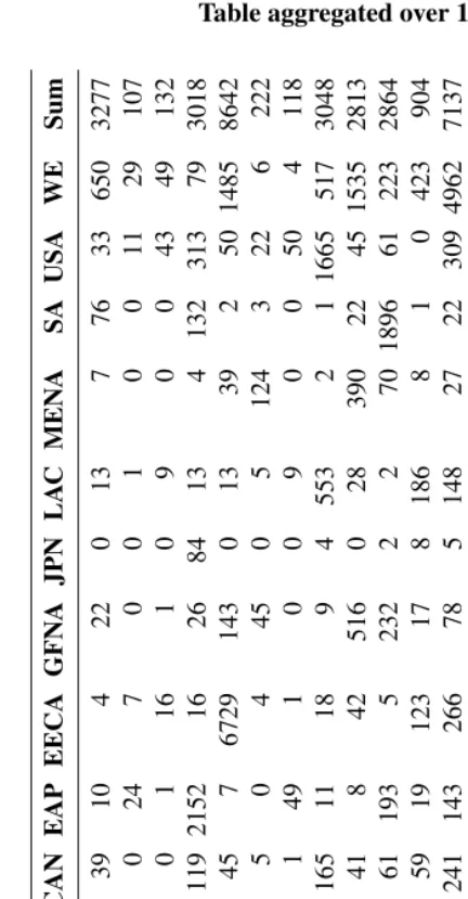
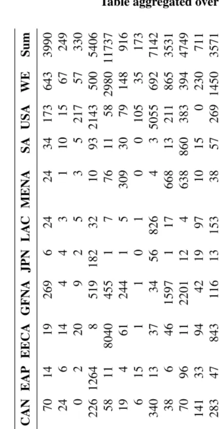
Table 8: 1960s estimated global migrant transition flow (in 1000’s) Table aggregated over 12 World Bank regions

(26)

(27)

(28)

(29)

Estimates of the total volume of migrant transition flows increase over time, reflecting global population growth. However, in both the 1970s and 1980s estimated flows between all countries were steady at around 42 million. The most popular origins of flows over the entire time period, by estimated volume, were in Eastern Europe and Central Asia (EECA) and, in the later tables, Latin America and the Caribbean (LAC). Most destinations of those in the EECA region tended to be to other countries also within the EECA region, whereas the flows out of LAC tended to go to other regions, most notably the USA. Large migrant transition flows are estimated from Western Europe (WE) and South Asia (SA) regions in the 1960s and 1970s tables respectively. The majority of these large flows are to other nations in the same region. The most popular destinations of flows over the entire time period, by estimated volume, were into the USA and WE. The largest sending regions into the USA were East Asia and the Pacific (EAP) and LAC. The largest flows into WE came from the east (EECA) and other WE nations.

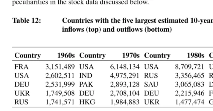
Results can also be studied on a country by country basis from the full migrant tran-sition flow tables. Table 12 shows the largest estimated inflows (top) and outflows (bot-tom) which are taken from the flow table column and row totals respectively. The USA received the highest estimated migrant transition inflows of any country in almost every decade (top of Table 12). Germany was also a large receiver of estimated inflows through-out each decade studied, whilst the United Kingdom and France were also top receivers in the 1990s. France received the largest inflow of all nations in the 1960s. Large mi-grant inflows to France during this decade were estimated to originate from Algeria, Italy, Spain and Portugal. Russia and the Ukraine also received large numbers of estimated immigrants in all decades with exception of the 1970s. India and Pakistan both received large estimated inflows during the 1970s, as did Saudi Arabia in the 1980s.

Russia was a top origin for estimated migrant transition outflows in each of the first three decades (bottom of Table 12), as was the Ukraine and Kazakhstan in the 1980s and 1990s respectively. The majority of these outflows are to other former USSR countries. For example, the large outflows from Kazakhstan in the 1990s are estimated to meet a large increase in the Kazakhstan-born stocks in Russia (1.8 to 2.5 million). The rise in the number of Kazakhstan-born in Russia alongside large flows from other former USSR countries such as Uzbekistan, the Ukraine and Azerbaijan created a large inflow in the 1990s into Russia. As illustrated in the methodology section, these estimates are ultimately based on changes in the stock data, which in this case originate from World Bank imputation rather than raw data from censuses or registers. Other nations in the former USSR and Indian sub-continent also have large estimated migration flows from big differences in stock imputations over time.

(30)

born in Poland (their stock falls from 474,000 to 280,000 between the start and end of the decade). In the 1990s the outflow is driven by migrants from Portugal and Spain returning to their place of birth (their stock falls from 609,000 and 429,000 to 141,000 and 151,000 respectively between the start and end of the decade). Germany has a large outflow of migrants in the 1980s. The largest estimated flow from Germany in this decade is to the Czech Republic, to match a large fall in the number of Czech born residents (from around 750,000 in 1980 to 375,000 in 1990). World Bank stock data for Germany, as with the former USSR nations were imputed, as no place of birth data was available. The large outflows from Turkey in the 1970s were also influenced by the stock data in Germany, where the number of Turkish born rose from around 440,000 in 1970 to 1.65 million in 1980. The large outflows from China in the 1990s were to the USA and Hong Kong. The appearance of China and Hong Kong as large senders in earlier decades might be due to peculiarities in the stock data discussed below.

Table 12: Countries with the five largest estimated 10-year migrant transition inflows (top) and outflows (bottom)

Country 1960s Country 1970s Country 1980s Country 1990s

FRA 3,151,489 USA 6,148,134 USA 8,709,721 USA 13,346,816 USA 2,602,511 IND 4,975,291 RUS 3,356,465 RUS 5,082,317 DEU 2,531,999 PAK 2,893,128 SAU 3,065,083 DEU 3,738,591 UKR 1,749,508 DEU 2,708,104 DEU 2,215,946 FRA 2,873,948 RUS 1,741,571 HKG 1,984,883 UKR 1,477,474 GBR 1,819,267

Country 1960s Country 1970s Country 1980s Country 1990s

RUS 3,086,746 BGD 4,800,661 RUS 2,655,499 MEX 5,037,273 HKG 1,500,636 IND 4,066,949 MEX 2,446,505 IND 2,594,894 PAK 1,440,894 RUS 2,117,101 IND 2,403,785 FRA 2,586,883 ITA 1,285,555 TUR 1,774,873 UKR 1,507,850 CHN 1,643,347 FRA 1,243,313 CHN 1,693,328 DEU 1,354,946 KAZ 1,605,811

(31)

Estimated values can be further explored by studying the place of birth dimension, alongside the origin and destination of migrant transition flows. For example, considering the USA as a destination, the largest estimated inflows by origin and place of birth in each decade are shown Table 13.

Table 13: Countries with the five largest estimated 10-year migrant transition inflows to the USA by origin and place of birth

Origin Destination Place of Birth

1960s Origin Destination Place of Birth

1970s

CUB USA CUB 439,346 MEX USA MEX 1,556,421

MEX USA MEX 402,118 PHL USA PHL 361,425

PRI USA PRI 343,996 KOR USA KOR 231,073

PHL USA PHL 142,902 PRI USA PRI 212,880

HKG USA CHN 85,868 CUB USA CUB 208,657

Origin Destination Place of Birth

1980s Origin Destination Place of Birth

1990s

MEX USA MEX 2,399,422 MEX USA MEX 4,910,358

PHL USA PHL 495,993 PHL USA PHL 54,1725

SLV USA SLV 407,537 IND USA IND 500,653

KOR USA KOR 383,622 VNM USA VNM 437,534

VNM USA VNM 329,061 CHN USA CHN 411,763

Notes: CUB = Cuba, MEX = Mexico, PRI = Puerto Rico, HKG = Hong Kong, PHL = Philippines, KOR= South Korea, SLV = Slovenia, VNM = Vietnam, IND = India, CHN = China.

(32)

re-ported 1.5 million Chinese born in Hong Kong. This stock drops to 16,823 in 1970 and rises back up to almost 1.9 million in 1980. This dramatic movement in the reported stocks creates a large estimated outflow of Chinese in the 1960s. These emigrants are moving to countries where there are increases in the number of Chinese born, including but not exclusively, China. In turn, during the 1970s there is a large inflow back into Hong Kong of Chinese born, to meet the sudden increase in their migrant stock.

4. Validation of results

Due to the large size of the estimated migrant flow tables, some form of dimension re-duction is required in order to asses estimates beyond looking at compressed tables of regional flows and the top inflows and outflows. In this section, the estimated migration transition flows from the applied methodology are discussed with reference to comparable estimates of global net migration flows of the United Nations and models for international migration.

4.1 Net migration comparison

The United Nations Population Division (2011) published net migration flows for each member country over a five-year period. These data are based predominately on scaled annual flows, derived from either migration records or through demographic accounting. In order to get a 10-year net migration flow, to correspond to the estimated 10-year mi-grant transitions, the two 5-year net migration flow totals for each decade (one for the first half of a decade and one for the second half) were summed for each country. A net rate was then calculated using the mid-decade population totals and multiplying by 1000. Comparative net migration rates from the estimates were calculated by taking the total in-flow away from total outin-flow in each country, divided by the mid-decade population totals and multiplying by 1000. A scatter plot comparing the estimated net rates (on the y-axis) with the derived United Nations net rate (x-axis) for each decade is shown in Figure 1.

There is a noticeable general linear trend along thex = y line, indicating a broad conformity of the estimated with the derived UN net rates. This relationship is confirmed in separate regressions for each decade of the estimated rate on the derived United Nations rate and an intercept, shown in Table 14. Parameters are estimated in R using therlm

(33)

Figure 1: Scatter Plot of Estimated Net 10-year Migrant Transition Flow Rates vs. Derived UN Rates (per 000). Countries labelled accord-ing to their ISO 3166-1 alpha-3 code (ISO, 2006)

●● ● ● ● ● ● ● ● ● ● ● ● ● ● ● ● ● ● ● ● ● ● ● ● ● ● ● ● ● ●● ●●● ● ● ●_●● ● ● ● ● ●● ● ● ●●● ●● ● ● ● ● ● ● ● ● ● ● ● ● ● ● ● ● ● ● ● ● ● ● ● ●●●●● ● ● ● ● ● ● ● ●● ● ● ● ● ● ● ● ● ● ● ● ● ● ● ● ● ● ● ● ● ● ● ● ● ● ● ●●● ● ●● ● ● ● ●●●● ●●●● ● ●●● ● ● ● ● ● ● ● ● ● ● ● ● ● ● ● ●●●●● ● ● ● ● ● ● _●●● ● ● ● ●●● ● ● ● ● ● ● ● ● ●● ● ● ●● ● ● ● ● ● ●● ● ● ● ● ● ● ● ● ● ● ● ● ● ● ● ● ● ● ● ●● ● ● ● ● ● ● ● ●● ●●● ● ● ●_●● ● ● ● ● ●● ● ● ●●● ●● ● ● ● ● ● ● ● ● ● ● ● ● ● ● ● ● ● ● ● ● ● ● ● ●●●●● ● ● ● ● ● ● ● ●● ● ● ● ● ● ● ● ● ● ● ● ● ● ● ● ● ● ● ● ● ● ● ●● ● ● ●●● ● ●● ● ● ● ●●●● ●●●● ● ●●● ● ● ● ● ● ● ● ● ● ● ● ● ● ● ● ●●●●● ● ● ● ● ● ● _●●● ● ● ● ●●● ● ● ● ● ● ● ● ● ●● ● ● ●● ● ● ● ● ● AFGALB DZA AGOARGARM ABW AUS AUT AZE BHS BHR BGD BRB BLR BEL BLZ BENBTN BOL BIHBWABRA

BRN

BGR

BFA BDIKHMCMR

CAN

CPVCAF TCDCHLCHN

COL

COMCODCOG_CRI CIV HRV CUB CYPCZE DNK DJI

DOMSLVEGYECU

GNQERI EST ETH FJI FIN FRA GUF PYF GAB GMB GEO DEU GHA GRC GRD GLP GTM_GIN

GNBGUYHNDHTI

HKG

HUN ISLINDIDNIRQIRN

IRL ISR ITA JAM JPN JOR KAZ KENPRK KOR KWT KGZ LAOLVA LBN LSOLBR LBY LTU LUX MAC

MKDMDGMWI

MYS MDV

MLI

MLT MTQ_MRT

MUSMEXMAR_ANTMNGMOZMMRNPLFSMNAMNLDMDA

NCL

NZL

NIC

NERNGANOR

OMNPANPAKPNG

PRYPHLPERPOL PRT PRI QAT REU ROU RUS_RWA WSM STP SAU SEN SCG SLE SGP SVK SVNESPSOMLKAZAFSLB

LCA VCT SURSDN

SWZ_SYRSWECHE

TWN TJK

TZA

THATLSTGO

TON TTO TUNTUR TKM UGA UKR ARE GBRUSA URYVNMVUTVENUZB

PSE

YEMZWEZMB

●●●●●● ● ● ● ● ● ● ● ● ●● ● ● ● ● ● ● ● ● ● ● ● ● ● ● ● ● ●●●● ● ● ●_● ● ● ●_● ●● ● ●● ● ● ● ● ● ● ●●● ● ● ● ● ● ● ● ● ● ● ● ● ● ● ●● ● ● ●●●●● ● ● ● ● ● ● ●●●_● ● ● ● ● ● ●● ● ●● ● ● ●●●● ●● ● ● ●● ● ● ● ●●● ● ●● ● ● ● ●●● ● ● ● ● ● ●●●● ● ● ● ● ● ● ● ● ● ● ●●●●●●●●● ● ● ● ● ● ● ● ● ● ● ●●●● ●● ● ● ●● ● ●● ● ●● ● ● ● ● ● ● ● ●● ●●●●●● ● ● ● ● ● ● ● ● ●● ● ● ● ● ● ● ● ● ● ● ● ● ● ● ● ● ●●●● ● ● ●_● ● ● ●_● ●● ● ●● ● ● ● ● ● ● ●●● ● ● ● ● ● ● ● ● ● ● ● ● ● ● ●● ● ● ●●●●● ● ● ● ● ● ● ●● ● ● ● ● ● ● ● ●● ● ●● ● ● ●●●● ●● ● ● ●● ● ● ● ●●● ●●● ● ● ● ●●● ● ● ● ● ● ●●●● ● ● ● ● ● ● ● ● ● ● ●●●●●●●●● ● ● ● ● ● ● ● ● ● ● ●●●● ●● ● ●●● ● ●● ● ●● ● ● ● ● ● ● ●●● AFGAGODZAALBARGARM

ABW AUS AUT AZE BHS BHR BGD BRB BLRBEL BLZ BEN BTN BOL BIH BWA BRA BRN BGR BFA BDI KHMCMR CAN CPV CAF TCDCOLCHLCHN

COM COD COG_HRV_CRICIV

CUB_CYPCZEDNK

DJI DOMECU EGY SLV GNQ ERI EST

ETH_FJIFINFRA GUF PYFGAB GMB GEO DEU GHAGRC GRDGLP GTM GIN GNB GUY HTI HND HKG

HUN_ISL_IRQIDNINDIRNITAIRLISR

JAM

JPN

JOR KAZKORKEN_PRK

KWT KGZ LAO LVA LBNLSO LBR LBY LTULUX MAC MKD

MDGMYSMDVMWI

MLIMLT MTQ MRT MUSMEX FSM MDA MNG

MARMMRMOZ NAMNPLNLD

ANT

NCL NZL

NICNERNORNGA

OMN PAK

PAN

PNG

PRYPERPHLPOL_PRT PRI

QAT

REU

ROURWARUS

WSM

STP

SAU

SENSCGSVKSLESGPESPSLBZAFSVN SOM

LKA

LCA VCT

SDN

SUR

SWZSYRCHESWETWNTJKTZATHA TLSTGO

TON

TTOUGATUNTURTKMUKR

ARE

GBRUSA URYVUTUZB VEN

VNM

PSE YEMZWEZMB

● ● ●●● ● ● ● ● ● ● ● ● ● ●● ● ●● ● ● ● ● ● ● ● ●● ● ● ● ● ●●●● ● ● ●●● ● ● ● ● ● ● ● ● ● ● ● ● ● ● ● ●● ● ● ● ● ● ● ● ● ● ● ●● ● ● ● ●●●●● ● ● ● ● ● ● ● ● ● ● ● ●● ● ● ● ● ● ● ● ● ● ● ● ● ● ● ● ● ● ● ● ● ●● ● ●●● ● ●● ● ● ● ● ● ● ● ● ● ● ● ●● ● ●_●● ● ● ● ● ● ● ● ● ● ● ● ● ● ● ● ● ● ● ● ● ● ● ● ● ● ● ● ● ●● ●●● ● ● ● ● ● ● ● ● ● ● ● ● ● ● ● ● ● ● ● ●● ● ● ●●● ● ● ● ● ● ● ● ● ● ●● ● ●● ● ● ● ● ● ● ● ●● ● ● ● ● ●_●●● ● ● ●●● ● ● ● ● ● ● ● ● ● ● ● ● ● ● ● ●● ● ● _{● ●} ● ● ● ● ● ● ●● ● ● ● ●●●●● ● ● ● ● ● ● ● ● ● ● ● ●● ● ● ● ● ● ● ● ● ● ● ● ● ● ● ● ● ● ● ● ● ●● ● ●●● ● ●● ● ● ● ● ● ● ● ● ● ● ● ●● ● ●_●● ● ● ● ● ● ● ● ● ● ● ● ● ● ● ● ● ● ● ● ● ● ● ● ● ● ● ● ● ●● ●●● ● ● ● ● ● ● ● ● ● ● ● ● ● ● ● ● ● ● ●●● AFG ALB

DZAAGOARG

ARM

ABW AUTAUS

AZEBHS BHR BGD BRB BLRBEL BLZ BENBTN BOL BIH BWA BRA BRN BGR

BFACMRKHMBDI

CAN

CPV CAF TCD_COLCHLCHN

COMCOD COGHRVCRICIV CUB

CYP CZE

DNK

DJI

DOMEGYECU SLV GNQ ERI EST ETH FJI FIN FRA GUF

PYFGABGMB

GEO

DEU

GHAGRC

GRD GLP

GTMGNBGIN

GUY HTI HNDHUNIDN IRNINDISLHKG

IRQ IRL ISR ITA JAM JPN JOR KAZKENPRKKOR

KWT KGZLAO LVA LBN LSO LBR LBY LTU LUX MAC MKD

MDG MWIMYS MDV MLI MLT MTQ MRT MUSMEX FSM

MDAMARMNG MOZ MMRNPLNAM

NLD

ANT

NCL NZL

NIC

NER_NGANOR

OMN

PAK

PANPNG PRY PER_PHLPOL PRT PRI QAT REU ROU RUS RWA WSM STP SAU SEN SCGSLE SGP SVK SVN SLB

SOM _LKAESPZAF

LCA VCT SDN SUR SWZ SWECHE

SYR_TJKTWNTZATGOTHATLS

TON TTO TUNTUR TKM UGA UKR ARE GBRUSA URY UZB

VUTVNMVEN PSEYEMZMBZWE

● ● ● ● ● ● ● ● ● ● ● ● ● ● ●● ● ● ● ● ● ● ● ● ● ● ● ● ● ● ● ● ●● ● ● ●_● ● ● ● ● ● ● ● ● ● ●● ● ● ● ● ● ● ● ● ● ● ● ● ● ● ● ● ● ● ● ● ● ● ● ● ● ● ● ● ● ● ● ●● ● ● ● ● ● ● ● ● ● ● ● ● ● ● ● ● ● ● ● ● ● ● ● ● ● ● ● ● ● ● ● ● ● ● ● ● ● ● ● ● ● ● ● ● ● ●● ● ● ●● ● ●● ● ● ● ● ● ● ● ● ● ● ● ● ● ● ● ● ● ● ● ● ● ● ● ● ● ● ● ●● ● ● ● ● ● ● ● ● ● ●● ●● ● ● ● ● ● ● ● ●● ● ● ● ● ● ● ● ● ● ● ● ● ● ● ● ● ● ● ●● ● ● ● ● ● ● ● ● ● ● ● ● ● ● ● ● ●● ● ● ●_● ● ● ● ● ● ● ● ● ● ●● ● ● ● ● ● ● ● ● ● ● ● ● ● ● ● ● ● ● ● ● ● ● ● ● ● ● ● ● ● ● ● ●● ● ● ● ● ● ● ● ● ● ● ● ● ● ● ● ● ● ● ● ● ● ● ● ● ● ● ● ● ● ● ● ● ● ●● ● ● ● ● ● ● ● ● ● ● ●● ● ●●● ● ●● ● ● ● ● ● ● ● ● ● ● ● ● ● ● ● ● ● ● ● ● ● ● ● ● ● ● ● ●● ● ● ● ● ● ● ● ● ● ●● ●● ● ● ● ● ● ● ● ●● ● ● ● ● AFG ALB

DZAARG_AGO

ARM ABW AUS AUT AZE BHS BHR BGD BRB BLRBEL BLZ BEN BTN BOL BIH BWA BRA BRN BGR_BFA

BDI CMRKHM

CAN CPV CAF TCDCHL CHN COL COMCOD COG CRI CIV HRV CUB CYP CZE DNKDJI DOMECU EGY SLV GNQ ERI EST ETH FJI FIN FRA GUF PYF GAB GMB GEO DEU GHA GRC GRD GLP GTM GIN GNB GUY HTI HND HKG HUN ISL IND IDN IRN_IRQIRL

ISR ITA JAM JPNJOR KAZ KEN PRK KOR KWT KGZ LAO LVA LBN LSO LBR LBY LTU LUX MAC MKD MDG MWI MDVMYS

MLI MLT MTQ MRT MUS MEX FSMMDA

MNGMAR MOZMMRNPLNLDNAM

ANT NCL NZL NIC NER NGANOR OMN

PAKPNGPAN PRY PERPHL POL PRT PRI QAT REU ROURUS RWA WSM STP SAU SEN SCG SLE SGP SVKSVN SLB SOM ZAF ESP LKA LCA VCT SDN SUR

SWZSWECHE

SYR TWN TJK TZA THA TLS TGO TON TTO

TUNTUR_TKMUGA

UKR

ARE

GBRUSA URY

UZB

VUTVNMVEN

PSE YEM ZMB ZWE 1960s 1970s 1980s 1990s −500 0 500 0 500 1000 −200 0 200 400 −200 0 200 400

−200 0 200 400 600 −500 0 500 1000

−400 −200 0 200 400 −300 −200 −100 0 100 200 300

United Nations Net Rate per 000

Estimated Net Rate per 000

(34)

esti-mated net rates in any of the four time periods. The slope coefficients are all positive, but less than unity, indicating the estimated net rates values are lower than the derived United Nations net rate. This result is not unexpected for three reasons. First, the United Nations net figures are based on timing definitions for migration during an interval that is less than 10 years. Subsequently more migrant transitions are recorded from moves over the periods of time. This difference is compounded when a 10-year net was derived. Second, the estimated 10-year migration tables represent transitions and not movements. Hence, multiple movements of a migrant might potentially be recorded by the United Nations over a five-year period, where only one transition comparing the location of the migrant at the start and end of the period is considered in the net rate based on the estimated flow tables. Third, the estimated data from the flow from stocks methodology are the minimal migration flow transitions in each decade required to meet the World Bank stock data. This minimum was derived by setting the diagonal values in each place of the birth table to their maximum value as illustrated in the methodology section.

Table 14: Regression of derived United Nations (UN) net rates on estimated net rates

Parameter (Std. Error) 1960s 1970s 1980s 1990s

Intercept 2.19803 -0.33207 -1.05609 -1.52908 (1.76241) (1.92035) (1.90238) (2.27249) UN Net Rate 0.53494 0.74672 0.64345 0.66924

(0.01721) (0.01508) (0.02244) (0.02919)

(35)

4.2 Gravity model

Kim and Cohen (2010) investigated non-economic predictors of reported international mi-gration bilateral flows. Using a log-normal regression model, geographic, demographic and social and historical determinants were estimated twice; once using migration flow data by origin into 17 destinations countries and once using migration flow data by des-tinations from 13 origin countries. Data were taken from the United Nations Population Division (2009), which published a set of unharmonised time series of sending and re-ceiving flow statistics reported by developed nations. Data for covariates were obtained from United Nations Population Division (2011) for demographic measures on popula-tion, potential support ratio (PSR), infant mortality rate (IMR), and urbanisapopula-tion, and the CEPII for geographic and social data on distances, language, and colonial relationships (Mayer and Zignago 2012).

In this section, the same initial model used in Kim and Cohen (2010) is fitted (once) to the logarithm of estimated bilateral flows between the 191 origin and destination coun-tries. Following the same procedures, estimated migration flows with value zero were excluded and logarithms with base 10 were used throughout. In addition, mid-decade values were taken for time varying covariate measures. The estimated parameters and standard errors are shown in Table 15 alongside the parameters obtained by Kim and Co-hen (2010) wCo-hen the model was fitted to the receiving data (K&C Receiving) and sending data (K&C Sending).

Standard regression diagnostics suggested there were no major problems with the model assumptions. What follows is a brief discussion of the parameter estimates, and comparisons with the results found by the two model fits of Kim and Cohen (2010). For further clarification on the expected direction and justification of variable constructions and selection, the reader is referred to Kim and Cohen (2010).

(36)

(as a fraction of the population totals) there are higher expected migration flows, when all other parameters are held constant. For the destination parameter, this result reflects a high number of estimated migrations from developing to developed countries. This result is of lesser importance for migration from origins where the parameter value is relatively close to zero when the standard error is considered. For destinations, similar results were found in both models based on the receiving and sending data in Kim and Cohen (2010). For the IMR, negative parameters suggest that at higher rates of infant mortality in either origin or destination the number of expected migration flows is lower. For destinations this effect is large, indicating that a destination with a high IMR is expected to have fewer immigrants, having controlled for all other variables. For origins this effect is relatively close to zero, again indicating slightly counter-intuitively that an origin with a high IMR is expected to have fewer emigrants. This can be explained by the inclusion of migration from the poorest countries, such as those in parts of Africa where there are low levels of education, migrant networks, and relatively high costs to migration, leading to very low numbers of movements. The percentages of urban population in the destination and origin increased the expected migration flows in and out of countries respectively, as expected.

For geographic determinants, both distance and an indicator variable for border shar-ing had large effects on the expected migration flow, especially in comparison with the Kim and Cohen (2010) parameters. Unsurprisingly the distance parameter is very close to negative one, as the same information was used in the offset term of (12) for the esti-mation of stocks from flows. Other geographic parameters on land area and landlocked follow the intuitive results found by Kim and Cohen (2010); larger countries send and receive more expected migration flows, while landlocked countries have lower expected migration flows due to higher transportation costs.

(37)

Table 15: Estimated parameters of M1 in Kim and Cohen (2010) in a regres-sion on the logarithm of various migration flow counts.

Parameter Estimate K&C Receiving K&C Sending

(Std. Error) (Std. Error) (Std. Error)

Constant 2.271 (0.141) -9.960 (0.231) -12.408 (0.258) Demographic determinants

Log population (destination) 0.206 (0.007) 0.601 (0.009) 0.372 (0.008) Log population (origin) 0.423 (0.007) 0.728 (0.006) 0.936 (0.011) Log potential support ratio

(destination)

-0.166 (0.055) -0.811 (0.069) -0.052 (0.024)

Log potential support ratio (origin)

-0.027 (0.054) 0.045 (0.020) 0.915 (0.079)

Log infant mortality rate (destination)

-0.704 (0.017) 1.007 (0.049) -0.783 (0.016)

Log infant mortality rate (origin)

-0.083 (0.017) -0.466 (0.013) 0.359 (0.054)

Log percentage of urban population (destination)

0.239 (0.018) 3.057 (0.072) 0.307 (0.021)

Log percentage of urban population (origin)

0.163 (0.017) 0.332 (0.017) 2.578 (0.077)

Geographical determinants Log distance between capi-tals

-1.026 (0.010) -0.819 (0.011) -0.660 (0.012)

Log land area (destination) 0.210 (0.005) 0.234 (0.008) 0.146 (0.007) Log land area (origin) 0.047 (0.006) -0.047 (0.005) 0.030 (0.009) Landlocked (destination) -0.073 (0.010) -0.610 (0.040) -0.086 (0.011) Landlocked (origin) -0.104 (0.010) -0.170 (0.009) -1.043 (0.038)

Border 0.737 (0.023) 0.077 (0.022) 0.096 (0.024)

Social and historical determinants

Common official language 0.264 (0.015) 0.138 (0.014) 0.346 (0.027) 9% minority speak same

language

0.325 (0.015) 0.266 (0.014) 0.003 (0.027)

Colony 0.686 (0.026) 0.427 (0.017) 0.747 (0.023)

(38)

5. Summary and discussion

In this paper, a methodology to estimate global migrant transition flow tables is illustrated in two parts. First, a methodology to derive flows from sequential stock tables was out-lined. Second, the methodology was applied to recently released World Bank migration stock tables to estimate a set of four decadal global flow tables. The results of the ap-plied methodology were discussed with reference to comparable estimates of global net migration flows of the United Nations and previous models for international migration flows.

The methodology outlined adds to the limited exisitng literature on linking migration flows to stocks. Rogers and von Rabenau (1971), Rogers and Raymer (2005) and Rogers and Liu (2005) focused on US Census place of birth data to estimate inter-state migration transitions. The first of these papers relies on a simplistic principal assumption of equal growth of stock totals in all regions. As a result, the application of the method outlined to the World Bank data produced many strange results, including negative migration flows. The second paper relies on aggregated stock populations by their place of birth, place of residence at timet−1, and place of residence at timet. This added dimension of required data negates its application to estimating international migration flows. This point is also valid for the third paper, which relies on information of migrant stocks disaggregated by their place of residence at timet−1, place of residence at timet, and age group.

(39)

the results presented in this paper could potentially be incorporated into projection models that age populations at 10-year intervals. If denser intervals are desired, such as five-year or single-year age intervals, new estimates would be required. These could be derived in one of two ways. Stock tables in non-census years could be estimated to create a larger set of sequential stock tables (within the same time frame), allowing flows between closer time periods to be obtained. Alternatively, one could adapt a method such as that outlined by Courgeau (1973) to convert 10-year estimates to shorter periods. If such estimates were derived, they could potentially be compared with flow data from countries that have a Census question on the place of residence one or five years prior to their Census night, forming another conceivable validation exercise.

The estimated flow tables are a first-of-a-kind set of comparable global origin desti-nation flow data. Estimates represent the minimum number of migration transition flows required to meet the foreign born stocks. As discussed in the introduction, bilateral flow tables have a number of advantages over currently available international migration data. Stock data are collected in the country of residence via census questions or details col-lected from population registers which capture a single transition between birthplace and country of current residence. However, the methodology outlined allows flows to be esti-mated on three dimensions; origin, destination and place of birth. Consequently, multiple typologies of movements such as primary migration, return migration or onward migra-tion flows of non-natives to a third country are estimated. Results from both validamigra-tion exercises appeared promising. The validation exercises allowed, as did the brief overview of the main results, the identification of unexpected flows. For most cases, further inves-tigation of these unexpected results was driven by large changes in the input stock data. In other cases, the methodology could be further expanded in a number of different ways to address the causes of these unexpected flows.

(40)

were controlled for using rather crude methods. More detailed data are likely to exist in some counties on the mortality by place of birth of foreign born migrants that may negate the need to distribute the total number of deaths proportionally. In addition, the estimation of the place of residence of newborns could be further developed to allow for moves outside their country of birth in these early years. Finally, the log-linear models with an offset have been used to estimate missing internal migration flow data. Alternative auxiliary data, to the distance measure used in this paper, could be utilised within the methodology outlined.

In conclusion, comparable international migration flow data are needed by researchers to better understand people’s movements and identify patterns. Policy makers can also use comparable international migration flow data to help forecast populations better, where migration can often play an important role. The methodology outlined in this paper pro-vides a relatively simple yet powerful technique to estimate global migration flow tables, exploiting newly available global stock data.

6. Acknowledgements

I would like to thank James Raymer, Nikola Sander, and Jack DeWaard for their com-ments on an earlier version of this paper and Joel Cohen for his recommendations con-cerning the validation exercises. I would also like to thank the reviewers and the Associate Editor for further suggestions on improving the paper.

Corrections:

On June 3, 2013 several typing mistakes were corrected on pages 521, 522, and on page 524.