Demographic Researcha free, expedited, online journal of peer-reviewed research and commentary
in the population sciences published by the Max Planck Institute for Demographic Research Konrad-Zuse Str. 1, D-18057 Rostock·GERMANY www.demographic-research.org
DEMOGRAPHIC RESEARCH
VOLUME 23, ARTICLE 26, PAGES 737-748
PUBLISHED 12 OCTOBER 2010
http://www.demographic-research.org/Volumes/Vol23/26/ DOI: 10.4054/DemRes.2010.23.26
Formal Relationships 11
Attrition in heterogeneous cohorts
James W. Vaupel
Zhen Zhang
This article is part of the Special Collection “Formal Relationships”. Guest Editors are Joshua R. Goldstein and James W. Vaupel.
c
°2010 James W. Vaupel & Zhen Zhang.
2 Proof 739
3 Discussion 740
4 Applications 740
4.1 The shape of the hazard of attrition in heterogeneous populations 740
4.2 Estimation of the rate of aging in a heterogeneous cohort 742
Formal Relationships 11
Attrition in heterogeneous cohorts
James W. Vaupel1,3 Zhen Zhang2,3
Abstract
In a heterogeneous cohort, the change with age in the force of mortality or some other kind of hazard or intensity of attrition depends on how the hazard changes with age for the individuals in the cohort and on how the composition of the cohort changes due to the loss of those most vulnerable to attrition. Here we prove that the change with age for the cohort equals the average of the change in the hazard for the individuals in the cohort minus the variance in the hazard across individuals. The variance captures the compositional change. This very general and remarkably elegant relationship can be applied to understand and to analyze changes with age in many kinds of demographic hazards, including, e.g., the lifetable aging rate or the intensity of first births.
1. Relationship
Letµ(x, z)denote the hazard of attrition (e.g., the force of mortality) at agexfor a cohort of individuals in a subpopulation with characteristicz; the subpopulation could consist of a single individual. Letg(z)denote the probability density function ofzat initial age zero, lets(x, z) = exp[−R0xµ(a, z)da]denote the survival function for the subpopulation with characteristiczand let¯s(x) =R−∞∞ s(x, z)g(z)dzdenote the survival function for the population as a whole. Then
(1a) µ˙¯(x) = ¯˙µ(x)−σ2 µ(x),
whereµ¯(x) =R−∞∞ µ(x, z)s(x, z)g(z)dz/¯s(x)is the average hazard of attrition for the population at agexas a whole,µ˙¯(x) =d¯µ(x)dx is the change in this hazard with age for the population as a whole at agex,µ˙(x, z) = dµ(x,z)dx is the change in the hazard of attrition with age for subpopulation with characteristiczat agex,
¯˙
µ(x) =R−∞∞ µ˙(x, z)s(x, z)g(z)dz/¯s(x)is the average change in the hazard of attrition for subpopulations at agex, andσ2
µ(x) =
R∞
−∞µ2(x, z)s(x, z)g(z)dz/¯s(x)−µ¯2(x)is
the variance at agexin the hazard of attrition across subpopulations.
A relationship similar to (1a) holds for the case of a characteristic that is discrete. Letπz(x)be the proportion of the subpopulation with characteristicz surviving at age
x, with πz(x) = πz(0) exp[−
Rx
0 µz(t)dt], where µz(x) is the hazard of attrition of
the subpopulation with characteristic z at age x and πz(0) is the proportion of the
subpopulation with characteristicz at the initial age. Then the average of mortality of the whole population is given by
¯
µ(x) =
P
zPµz(x)πz(x)
zπz(x)
and
(1b) µ˙¯(x) = ¯˙µ(x)−σ2µ(x),
where µ¯˙(x) =
P
zPµ˙z(x)πz(x)
zπz(x) and σ
2 µ(x) =
P
zPµ2z(x)πz(x) zπz(x) −µ¯
2(x).
Equation (1b) is essentially the same as (1a) and can be used to study attrition in a population that is heterogeneous with regard to a discrete characteristic.
2. Proof
Becauseµ¯(x) =R−∞∞ µ(x, z)s(x, z)g(z)dz/¯s(x), it follows that
˙¯
µ(x) =
R∞
−∞{µ˙(x, z)s(x, z) +µ(x, z) ˙s(x, z)}g(z)dz
¯
s(x) −µ¯(x)
˙¯
s(x) ¯
s(x).
Substitutings˙(x, z) =−µ(x, z)s(x, z)ands˙¯(x) =−µ¯(x)¯s(x)and simplifying yields
˙¯
µ(x) = ¯˙µ(x)−
R∞
−∞µ2(x, z)s(x, z)g(z)dz
¯
s(x) + ¯µ 2(x)
= ¯˙µ(x)−σ2µ(x). Q.E.D.
Equation (1b) can be proven in a similar manner. Simple calculus yields
˙¯
µ(x) =
P
z( ˙µ(x)πPz(x) +µz(x) ˙πz(x))
zπz(x) −µ¯(x)
P
zπ˙z(x)
P
zπz(x).
Becauseµz(x) = −π˙z(x)/πz(x), it follows thatπ˙z(x) = −µz(x)πz(x). Substituting
this expression into the above equation leads to
˙¯
µ(x) = ¯˙µ(x)−σ2
µ(x) Q.E.D.
Equation (1a) - and with minor modifications equation (1b) - can also be proven as a special case of the more general equation
(2) v˙¯(x) = ¯˙v(x) +Cov(v(x), r(x)).
In (2),v(x, z)gives the value of some function of age or timexin the subpopulation with characteristicz, the proportion of individuals at age or timexin the subpopulation with characteristiczis given by the probability density functiong(x, z),
¯
v(x) =R−∞∞ v(x, z)g(x, z)dz, v˙¯(x) = d¯v(x)dx , v˙(x, z) = dv(x,z)dx and
¯˙
The covariance is given by
Cov(v(x), r(x)) =
Z ∞
−∞
v(x, z)r(x, z)g(x, z)dz−¯v(x)¯r(x),
wherer(x, z) =dg(x,z)/dxg(x,z) is the relative derivative of the density function and
¯
r(x) =R−∞∞ r(x, z)g(x, z)dz. To prove (1a), substituteµforvin (2) and substitute s(x, z)g(z)/s¯(x)forg(x, z). It readily can be shown thatr(x, z) =−µ(x, z) + ¯µ(x). It follows thatCov(v(x), r(x)) =−σ2
µ(x).
3. Discussion
Equation (1) is very general. In the frailty model developed by Vaupel, Manton, and Stallard (1979), an individual’s frailty is a relative-risk that is fixed for life, and in many applications frailty is assumed to be gamma distributed. Equation (1), however, holds regardless of the distribution ofzand even ifzis not a relative-risk (proportional-hazard) butzaffects the hazard of attrition in some complicated manner. The value ofzcan be positive, zero or negative. Every individual in the population could have a unique value of zthat determines the mortality trajectory over age for that individual. Depending on the individual, such trajectories could rise or fall or rise and then fall, etc. Changing-frailty models in which an individual’s risk varies with age, perhaps stochastically, can be captured by definingzas an index of every possible trajectory.
Both (1) and (2) were presented at an annual meeting of the Population Association of America (Vaupel 1992). A proof of (2) is given by Vaupel and Canudas-Romo (2002). A version of (2) without the first term on the right was derived by Preston, Himes and Eggers (1989). A discrete version of (2) was devised by Price (1970) to analyze genetic change. Cohen (1971) independently derived the same result. Coulson and Tuljapurkar (2008) extend the so-called Price equation.
4. Applications
4.1 The shape of the hazard of attrition in heterogeneous populations
Consider the simplest case where the hazard of attrition for individuals is constant over age but varies across individuals. Thenµ˙(x) = 0andµ¯˙(x) = 0, resulting in
˙¯
µ(x) =−σ2
µ(x)<0for allx. That is, the hazard of attrition for the overall population
If the hazard of attrition for subpopulations is decreasing with age (i.e. µ˙(x, z)<0
andµ¯˙(x)< 0), the hazard of attrition for the population as a whole must decease with age, because both terms on the right hand side of (1),µ¯˙(x)and−σ2
µ(x), are negative.
This result is well known in reliability theory (e.g., Barlow 1985, Proschan 1963). The case of increasing mortality for individuals, however, is not so simple: the average hazard of attrition for the population as a whole could either increase or decrease at age xdepending on the value of µ¯˙(x) vs. σ2
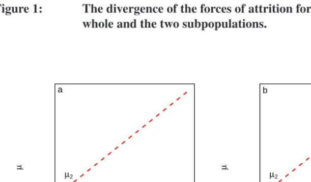
µ(x). As an example, consider a population
composed of two subpopulations with forces of attritionµ1(x) =c1t+a1and
µ2(x) =c2t+a2, with0< c1< c2and0< a1< a2. Then the hazard of attrition for the
overall population can decrease over some ages and increase over other ages, as shown in Figures 1a and 1b.
Figure 1: The divergence of the forces of attrition for the population as a whole and the two subpopulations.
x
µ
a
µ2
µ1
µ
x
µ
b
µ2
µ1
µ
Note: The blue dotted line representsµ1(x) =c1t+a1withc1=.5anda1=.1, the red dashed
lineµ2(x) =c2t+a2withc2= 2anda2= 3. The solid line represents the force of attrition
for the population as a whole. The only difference between the two figures is that the share of the subpopulation withµ1(x)at initial age zero is .1 in Figure 1a and .5 in Figure 1b. The graph in
The pattern of attrition for the population as a whole can differ from the patterns for subpopulations or individuals in a variety of ways, as illustrated by Vaupel and Yashin (1985). The above examples illustrate how equation (1) can shed light on patterns of attrition in heterogeneous populations.
4.2 Estimation of the rate of aging in a heterogeneous cohort
A more specific application of equation (1) is in studies of the rate of aging, measured as the relative change with age in the force of mortality. Note that dividing both sides of (1) byµ(x)¯ yields the relative change in the force of mortality for the whole population:
(3) ¯b(x) = d¯µ(x) ¯ µ(x)dx = ¯˙ µ(x) ¯ µ(x)− σ2 µ(x) ¯
µ(x) =b
†(x)−µ(x)CV¯
µ(x)
where
b†(x) = µ(x)¯˙ ¯ µ(x) =
R∞
−∞
dµ(x,z)/dx
µ(x,z) µ(x, z)s(x, z)g(z)dz/¯s(x)
R∞
−∞µ(x, z)s(x, z)g(z)dz/¯s(x)
is the deaths-weighted rate of aging (because the density of deaths is given by the product ofµands) andCVµ(x) =σµ2(x)/µ¯2(x)is the coefficient of variation at agex.
Suppose the force of mortality is given byµ(x, z) = zaexp(bx) +c with frailtyz
at initial age zero described by a gamma distribution with mean 1 and varianceγ. Then, results in Vaupel, Manton and Stallard (1979) imply that:
(4) µ(x) = ¯¯ z(x)(µ(x,1)−c) +c= aexp(bx)
1 +aγb (exp(bx)−1)+c,
wherez(x)¯ is the mean value of frailty among survivors at agex. It appears that such a logistic curve may capture the pattern of human mortality from age 35 or so to the most advanced ages (Thatcher, Kannisto and Vaupel 1998, Vaupel 2010). It can be readily shown thatµ(x) =¯˙ b(¯µ(x)−c). Furthermore, because (4) can be rearranged as
¯
µ(x)−c= (µ(x,1)−c)¯z(x), it follows thatσ2
µ(x) =γ(¯µ(x)−c)2, where
γ=σ2
These results, substituted in (3), imply:
(5) ¯b(x) = µ˙¯(x) ¯
µ(x) =b
µ
1− c ¯
µ(x)
¶
−γ µ
1− c ¯
µ(x)
¶
(¯µ(x)−c),
where the relative derivative¯b(x)is the lifetable aging rate (Horiuchi and Coale 1990, Horiuchi and Wilmoth 1997, 1998).
The curve in (4) asymptotically approaches a limit ofµ¯∗=b/γ+c. In recent decades
for countries with high life expectancies, it appears that this limit is closely approached by age 110, such that the force of mortality after 110 is essentially constant at a value of about .7, which implies an annual probability of death of about50%(Gampe 2010). In any case, at the limit (4) indicates:
(6) ¯b(x) = 0 =b µ
1− c ¯
µ∗
¶
−γ µ
1− c ¯
µ∗
¶
(¯µ∗−c),
which in turn impliesγ=b/(¯µ∗−c). Substituting this result in (5) yields:
(7) ¯b(x) =b
µ
1− c ¯
µ(x)
¶ µ
¯
µ∗−µ¯(x) ¯
µ∗−c
¶ .
Equation (7) shows how and why the lifetable aging rate¯b(x)differs from the rate of increase in mortalityb, which is constant for all the members of the population. The first adjustment tobreduces the value of¯b(x)at younger ages whencaccounts for a substantial share of total mortality. The second adjustment tobreduces the value of¯b(x)at older ages as the force of mortality approaches its maximum valueµ¯∗. Ifcis small compared with
this maximum value, then the adjustment is approximately equal to(1−µ(x)¯µ¯
∗ ). At the
maximum value¯b(x)equals zero. Note that becauseµ¯(x)≥c, both factors adjustingb are less than or equal to one. Hence,¯b(x) ≤b, and sometimes¯b(x)can be much lower thanb.
For Japanese females in 1980-2008, the force of mortality from age 50 to 105 can be serviceably approximated, using methods of maximum likelihood estimation, by (4) with initial age zero corresponding to chronological age 50, witha=.0007at the initial age, b = .14,c = .002andγ =.19; these values imply thatµ¯∗ = .73. For Swiss females
in 1860-1880, the parameter estimates area= .0018,b = .11,c = .007,γ =.15and
¯
µ∗ =.76. The trajectory of¯b(x)estimated by (7) resembles the trend of change in the
Figure 2: Lifetable aging rate for Swiss females in 1860-1880 (a) and for Japanese females in 1980-2008 (b).
40 50 60 70 80 90 100
0.00
0.05
0.10
0.15
Swiss females 1860−1880
Age
Lif
etab
le aging r
ate
a
50 60 70 80 90 100
0.00
0.05
0.10
0.15
Japanese females 1980−2008
Age
Lif
etab
le aging r
ate
b
Note: The black circles represent empirical lifetable aging rates calculated directly from the data and the red line represents the lifetable aging rate estimated by (7).
Source of data: Human Mortality Database available at http://www.demogr.mpg.de.
Consider, for instance, the attrition of childless women when they give birth. Suppose that in such a cohort, some of the women are married and the rest are not married. Suppose the intensity (i.e., force or hazard) of a first birth is higher for the married women than for the unmarried women, and suppose that the women are at an agexat which the intensity is rising for both groups. To be specific, suppose that half of the women are in each group, that for the married µm(x) = .5 andµ˙m(x) = .02 and that for the unmarried
µu(x) =.1andµ˙u(x) =.02. Thenµ¯˙(x) =.02andσµ2(x) =.04. Equation (1) indicates
References
Barlow, R.E. (1985). A Bayes explanation of an apparent failure rate paradox. IEEE Transactions on Reliability34(2): 107–108. doi:10.1109/TR.1985.5221964.
Block, H.W., Li, Y., and Savtis, T.H. (2003). Initial and final behavior of failure rate functions for mixtures and functions. Journal of Applied Probability40(3): 721–740.
doi:10.1239/jap/1059060898.
Cohen, J.E. (1971). Legal abortions, socioeconomic status, and measured intelligence in the United States. Biodemography and Social Biology 18(1): 55–63.
doi:10.1080/19485565.1971.9987900.
Coulson, T. and Tuljapurkar, S. (2008). The dynamics of a quantitative trait in an age-structured population living in a variable environment. The American Naturalist
172(5): 599–612.doi:10.1086/591693.
Finkelstein, M.S. (2009). Understanding the shape of the mixture failure rate (with engineering and demographic applications). Applied Stochastic Models in Business and Industry25(6): 643–663. doi:10.1002/asmb.815.
Gampe, J. (2010). Human mortality beyond age 110. In: H. Maier, J.G.B. Jeune, J.M. Robine, and J.W. Vaupel (eds.)Supercentenarians. Heidelberg: Springer: 219–230.
doi:10.1007/978-3-642-11520-2_13.
Horiuchi, S. and Coale, A.J. (1990). Age patterns of mortality for older women: An analysis using age-specific rate of mortality change with age.Mathematical Population Studies2(4): 245–267. doi:10.1080/08898489009525312.
Horiuchi, S. and Wilmoth, J.R. (1997). Age patterns of the life-table aging rate for major causes of death in Japan, 1951-1990. Journal of Gerontology: Biological Sciences
52A(1): B67–B77.doi:10.1093/gerona/52A.1.B67.
Horiuchi, S. and Wilmoth, J.R. (1998). Deceleration in the age pattern of mortality at older ages.Demography35(4): 391–412. doi:10.2307/3004009.
Preston, S.H., Himes, C.L., and Eggers, M. (1989). Demographic conditions responsible for population aging.Demography26(4): 691–704. doi:10.2307/2061266.
Price, G.R. (1970). Selection and covariance. Nature 227: 520–521.
doi:10.1038/227520a0.
Proschan, F. (1963). Theoretical explanation of observed decreasing failure rate.
Technometrics5(3): 375–383.doi:10.2307/1266340.
to 120. In:Monographs on Population Aging 5. Odense, Denmark: Odense University Press. Http://www.demogr.mpg.de.
Vaupel, J.W. (1992). Analysis of population changes and differences: Methods for demographers, statisticians, biologists, epidemiologists, and reliability engineers. Paper presented at the PAA Annual Meeting, Denver, Colorado, April 30 - May 2. Vaupel, J.W. (2010). Biodemography of human ageing. Nature 464: 536–542.
doi:10.1038/nature08984.
Vaupel, J.W. and Canudas-Romo, V. (2002). Decomposing demographic change into direct vs. compositional components. Demographic Research 7(1): 1–14.
doi:10.4054/DemRes.2002.7.1.
Vaupel, J.W., Manton, K.G., and Stallard, E. (1979). The impact of heterogeneity in individual frailty on the dynamics of mortality. Demography 16(3): 439–454.
doi:10.2307/2061224.
Vaupel, J.W. and Yashin, A.I. (1985). Heterogeneity’s ruses: Some surprising effects of selection on population dynamics. The American Statistician 39(3): 176–185.