Volume 24 - Article 34 | Pages 831–854

in the population sciences published by the Max Planck Institute for Demographic Research Konrad-Zuse Str. 1, D-18057 Rostock · GERMANY www.demographic-research.org

DEMOGRAPHIC RESEARCH

VOLUME 24, ARTICLE 34, PAGES 831-854

PUBLISHED 28 JUNE 2011

http://www.demographic-research.org/Volumes/Vol24/34/ DOI: 10.4054/DemRes.2011.24.34

Research Article

A dynamic extension of the period life table

Frank T. Denton

Byron G. Spencer

© 2011 Frank T. Denton & Byron G. Spencer.

This open-access work is published under the terms of the Creative Commons Attribution NonCommercial License 2.0 Germany, which permits use, reproduction & distribution in any medium for non-commercial purposes, provided the original author(s) and source are given credit.

1 Introduction 832

2 The period life table 833

3 Dynamic extension 834

4 Diagrammatic depiction 835

5 A note on interpretation 836

6 Age-independent changes in mortality 837

7 Application 839

8 Life expectancy and mortality prediction 843

9 Conclusion 844

10 Acknowledgements 845

References 846

A dynamic extension of the period life table

Frank T. Denton1

Byron G. Spencer2

Abstract

The standard period life table is based entirely on the death probabilities of the given period. Popular (not expert) usage of life expectancies from a period table typically ignores the fact that the expectancies make no allowance for future declines in mortality rates. But the historical record provides overwhelming evidence to suggest that declines will continue, and the period expectancies can therefore be misleading, in a practical context. We propose a “dynamic” extension of the period table that draws out the implications, for survivorship and life expectancy, of observed rates of change of death probabilities.

1 _{Frank T. Denton, M.A., LL.D. Research Institute for Quantitative Studies in Economics and Population and} Department of Economics. McMaster University. Hamilton, Ontario L8S 4M4.

Telephone: 905-525-9140-24595. Fax: 905-521-8232. E-mail: [email protected].

2 _{Byron G. Spencer, PhD. Research Institute for Quantitative Studies in Economics and Population and} Department of Economics. McMaster University. Hamilton, Ontario L8S 4M4.

1. Introduction

The life table is a time-honoured and useful device for studying the implications of observed mortality rates in a population (Standard references include Chiang 1984; Keyfitz 1968; Keyfitz and Caswell 2005; Kintner 2004; among others.) The period life table, by far the most common form, is based on the rates for a particular year, or averages over a few consecutive years. What the table does is to provide the probabilities of dying and their implications for survivorship, including the expected years of life remaining at different ages. What it does not do, and is not intended to do, is to allow for changes in mortality probabilities. All calculations are based on the probabilities of the given period.

The mean expectations of remaining years of life – life expectancies, as they are commonly termed – are frequently cited and used in practical contexts, and only seldom (in popular usage) is it pointed out that they imply no further reduction of mortality. But the history of mortality rates asserts a likelihood to the contrary. The historical record in developed countries reveals continuous declines for as far back as modern statistical record-keeping allows.3 _{We propose an extension of the period table that would allow}

explicitly for the possibility of further declines. We refer to it as a “dynamic” extension, and the life expectancies associated with it as “dynamic life expectancies.” The kernel idea is captured by comparing the following statements:

The period life table draws out the implications for survivorship and life expectancy of the observed age-specific mortality probabilities of a given period, under the assumption that the probabilities remain constant.

The dynamic extension of the period life table draws out the implications for survivorship and life expectancy of the observed mortality probabilities of a given period and the observed rates of change of those probabilities, under the assumption that the rates of change remain constant.

The extension is not proposed as a replacement for the period life table, nor should it be interpreted as providing an explicit forecast. It is intended rather as an optional

supplement to the standard table. Calculations of dynamic life expectancies are “what if” calculations: “what if” observed rates of change were to continue? In that sense they can be compared with the “what if” implications of the standard period life expectancies: “what if” mortality rates were to remain unchanged?

We note briefly the mathematics of the standard period life table and then develop the dynamic framework. We offer some general observations on the interpretation of the framework in the context of previous literature on the modeling of mortality rates and provide a more specific comparison with earlier work on age-independent changes in mortality. We show how the framework can be represented by an augmented Lexis diagram and illustrate dynamic life expectancy by an application to Canadian data, including comparisons of alternative dynamic expectancies with published 2001 period expectancies. We emphasize that the calculated death rates underlying the dynamic expectancies should be interpreted as "what if" calculations, not as forecasts.

2. The period life table

,1,...,

Consider a cohort of newborn children observed, as it grows older, at exact ages 0

x= m, where m is the oldest age at which there are any survivors. Let be the l0

initial size of the cohort (an arbitrary number) and let l_x be the number surviving to age x. The probability that a survivor to age x will die in the interval x to x+1 is constant at q_x

)

and an entry in the sequence , , …, can be calculated recursively from

1

l l₂ l_m

(

1 1

x = −q lx x

l₊ , or directly from l_x+1=l₀

∏

(

)

x to

Let Lx be the number of person-years lived in the interval x+1 and write , where

(

)

x

L = f f denotes an interpolation function, the form of which depends on the pattern of deaths in the interval. If deaths occur uniformly then f is linear and

(

)

x x

3. Dynamic extension

Let x stand again for exact age (with bounds 0 and ) but refer to it now as initial age. Let stand also for age and refer to it as subsequent age, with

m

y y≥x

n

. Assume there are period life tables for two periods (years) years apart, and refer to the more recent one as the reference period. Let q_x be the death probability at age x in the reference period table and let qx be the corresponding probability in the earlier period table. The annual rate of change for any age x is then rx =

(

)

y

xx

l , the first entry in the cohort sequence l_xx,

, 1

x x

l + , …, lxy. We refer to the cohort as the lxx cohort.) Assuming constancy of the death probability rate of change at each age, the probability that a member of the lxx cohort who has survived to age will die in the interval to y y y+1 is then

(

)

xy = y +

q q , where q_y is the death probability at age in the reference period, y

y

r is the annual rate of change of that probability, and y x− is the number of years elapsed in time (as well as age) since the cohort was of age x, and hence the number of years over which the age probability has changed. The cohort sequence of y l_xy values

(

)

(

)

directly from

+

(

)

, 1 1

y

x y x

l + =lx

∏

Now let L_xy (the dynamic analogue of L_x) stand for the number of person-years lived by survivors of the l_xx cohort in the interval to y y+1. Adapting the notation used earlier, . As before, if the pattern of deaths is uniform in the

interval, then the interpolation function

(

)

xy x y

L = f l ₊

f is linear, and L_xy=

(

)

. The total

x

q

lnqx qx

x

q

4 _{This is our preferred representation of the rate of change of for present purposes. An alternative would}

number of person-years yet to be lived by the lxx cohort is

m

xx _{t x} xt

T =

∑

There are thus two innovations on which the dynamic extension is based. The first is that each lx entry in the period table is redefined as lxx, the initial value of a separate cohort, with its own age sequence of death probabilities. The second is that the no-change assumption about death probabilities in the period table is replaced with the “what if” assumption that the observed rates of change since a previous period table will continue for as long as there are any survivors of a cohort.

4. Diagrammatic depiction

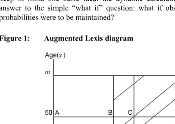
The framework for the dynamic extension can be represented in the form of an augmented Lexis diagram, as in Figure 1. Age is measured in the vertical dimension, time in the horizontal dimension. For convenience we choose 0 as the date (year) of the reference life table, and thus − as the date of the earlier table. With the scaling of age (

n

x) and time ( ) equal, the upward-sloping 45 degree lines represent the remaining age/time life paths of the cohorts (

t

1

+

m lxx) defined by the reference table and the horizontal lines represent the time paths of death probabilities (q_x

50

q

50 xy

). For example the line AB represents the -year interval over which the annual rate of change of is calculated. BC, the extension of AB, then represents the 10-year interval over which that annual rate of change is applied (by compounding over the ten years) to arrive at the value for the survivors of the cohort of initial age 40 when (10 years later) that cohort is of age 50. (The application of the death probability to the cohort survivors occurs at the intersection point C. In the “dynamic” notation, the number of cohort survivors at that point is and the death probability is

n xy l = 50 q 40,50 q q 40,

l = .) Similarly the line BD represents the interval over which the same annual rate of change is applied (by compounding over 50 years) to arrive at the value for the survivors of the cohort of initial age 0 when (50 years later) that cohort is of age 50. Note that if n

(so that the first two vertical lines coincide) the annual rate of change calculation is nullified and the diagram reduces to a simple depiction of the standard period life table: the set of death probabilities in the reference table then remains constant through time for each cohort and the probabilities lie on the vertical line passing through the point B. Note further, for another comparison, that if the rates of change of death probabilities over the n-year interval between the original life tables are simply used as an extrapolative device to move the time 0 probabilities forward another 10 years, say,

50

q

then a new life table can be generated at time 10. The new death probabilities would then lie on the vertical line passing through the point C in the diagram, rather than on the cohort-specific diagonal lines. The difference between the dynamic calculations and this simple extrapolative procedure is that the former assumes the rates of change will continue to compound, for each age cohort, for as long as there are any survivors of that cohort, while the latter makes no such assumption – it treats the changes as representing a one-time shift in the schedule of death probabilities. In all of this it is important to keep in mind one basic idea: the dynamic calculations are intended to provide an answer to the simple “what if” question: what if observed rates of change in death probabilities were to be maintained?

Figure 1: Augmented Lexis diagram

5. A note on interpretation

( )

f x

( )

the distinction between “senescent mortality” (associated with aging) and “background mortality” (independent of age); see Bongaarts (2009) for discussion. (In the Gompertz or similar sigmoid-type representation of mortality, with discrete age,

, where α is the background or baseline component and

lnqx =lnα+ f x is the senescence component; historically, continuing declines in α have been associated with consistently rising human life expectancy.) Model life table systems take advantage of the regularities in mortality patterns by reducing their representation to a small number of parameters that make it possible to generate complete tables from limited empirical information.5 _{All of this work is interesting in itself but different in nature and purpose}

from the contribution of the present paper. We mention it simply for comparison with our proposed extension of the standard life table and the drawing out of implications of observed changes in mortality rates for life expectancy, were they to be maintained.

We note also the following: Our procedure applies to cohorts and their death probabilities. In a population projection context one might think in terms of cohorts also but there one would need to specify death rates for all cohorts, including those born throughout the projection period. In our case the concern is with only those cohorts defined (implicitly) by the reference life table, and with death probabilities only for as long as there are any survivors of those cohorts. The death probabilities of as yet unborn cohorts are irrelevant.

6. Age-independent changes in mortality

The effects of age-independent changes in mortality rates have been studied in the context of the stable population model by Coale (1963), Coale and Demeny (1967), Keyfitz (1977), and Keyfitz and Caswell (2005). Two assumptions are considered by Keyfitz and Caswell: (a) uniform arithmetic changes in rates and (b) uniform proportional changes. The second assumption is the more realistic of the two (as the authors point out) and we focus on it. The Keyfitz and Caswell analysis is in a continuous time framework but we adapt it to the discrete time framework that we use here, for comparison with our proposed “dynamic” calculations.

Consider then an age schedule of population mortality rates, or more consistently for our purposes, death probabilities, q_x (x=0,1,...,m). Now (following Keyfitz and Caswell) suppose that the death probability at each age changes by the same fraction δ

k

each year, yielding after years a new schedule *

(

)

x x

q = +kδ q (x=0,1,...,m). (kδ must exceed − for the calculation to make sense.) Assuming the same initial input in both cases, the corresponding number of survivors at any age

1 l0

1

x+ is then

(

)

(

(

)

)

* *

0

0 0 1 1

x x

1 0 1

x+ =

∏

∏

l l q , which can be expressed as a polynomial in δ of degree x+1. Also adapting our earlier notation, we can write

and

(

)

1 x lx+ =

* _,

x

L f l * * *

x x x

e =T l . If f denotes a linear function it is easily shown that

both *

x

e and *

x x

e −e can be expressed as polynomials in δ of degree mfor every x (assuming the terminal probability is fixed at 1). A new period life table can be derived from the

m

q

*

x

q probability schedule, representing a new stationary population. Now consider for comparison, the assumption of age-independent rates of change in death probabilities in the context of our dynamic extension of the period life table. Using our earlier notation, that assumption implies the special case rx =r for all , so x that qxy =qy

(

)

requires , or

(

(

)

(

)

1 1

δ − δ

(

)

)

(

)

= + − − .) Unlike the

model used by Keyfitz and Caswell, the rate of change is thus compounded, and compounded separately for each of the m cohorts implicit in the life table (excluding the age m cohort with fixed at 1). Carrying through the substitution to the calculation of

m

q

, 1

x y

l + yields a polynomial in r of degree y x− , and carrying the

substitution further, to Lxy and Txx, leads to expressions for exx and exx−ex that can be interpreted as polynomials in rof degreem x− . (The polynomials are of degree rather than m since, unlike the period life table,

m x− x

xx

7. Application

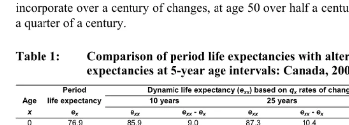
Examples are provided in Tables 1 and 2. The period life expectancies at five-year age intervals from 0 to 100 are taken from the Statistics Canada life tables for 2001 (based on average data for the three-year period 2000-2002) and compared with three dynamic life expectancies. Comparisons are shown for males in Table 1, females in Table 2. Complete single-age comparisons are provided in the Appendix; they are shown in graphical form as differences between dynamic and period life expectancies, in Figure 2. The dynamic expectancies are calculated using average rates of change of q_x values over the previous 10, 25, and 50 years.6 _{The younger the age, the longer the period over}

which changes in death probabilities take place. The oldest age at which there are any survivors in the calculations exceeds 100: thus at age 0 the dynamic expectancies incorporate over a century of changes, at age 50 over half a century, and at age 75 over a quarter of a century.

Table 1: Comparison of period life expectancies with alternative dynamic life expectancies at 5-year age intervals: Canada, 2001, males

Period Dynamic life expectancy (exx) based on qx rates of change in the previous --

Age life expectancy 10 years 25 years 50 years

x ex exx exx - ex exx exx - ex exx exx - ex

0 76.9 85.9 9.0 87.3 10.4 84.1 7.2 5 72.4 81.0 8.5 82.2 9.8 79.1 6.7 10 67.5 75.5 8.0 76.6 9.1 73.7 6.2 15 62.5 69.9 7.4 70.9 8.4 68.2 5.6 20 57.7 64.5 6.8 65.4 7.6 62.8 5.1 25 53.0 59.1 6.2 59.9 6.9 57.5 4.6 30 48.2 53.7 5.5 54.3 6.2 52.2 4.1 35 43.4 48.3 4.9 48.8 5.4 46.9 3.5 40 38.6 42.9 4.2 43.3 4.6 41.6 3.0 45 34.0 37.5 3.6 37.8 3.8 36.5 2.5 50 29.4 32.3 2.9 32.5 3.1 31.4 2.0

xy

6 _{The dynamic calculations are as described in a previous section. To allow for possible nonuniformity in the} distribution of deaths within a one-year age interval we did the following. For each period table we first calculated L by simple averaging L_xy=

(

)

x

and then multiplied it by a correction factor equal to

Table 1: (Continued)

Period Dynamic life expectancy (exx) based on qx rates of change in the previous --

Age life expectancy 10 years 25 years 50 years

x ex exx exx - ex exx exx - ex exx exx - ex

55 25.0 27.2 2.2 27.4 2.4 26.6 1.5 60 20.8 22.4 1.6 22.6 1.7 22.0 1.2 65 17.0 18.0 1.1 18.2 1.2 17.8 0.8 70 13.5 14.1 0.6 14.2 0.8 14.0 0.5 75 10.3 10.6 0.3 10.8 0.4 10.7 0.3 80 7.7 7.8 0.1 7.9 0.2 7.9 0.2 85 5.5 5.5 0.0 5.6 0.1 5.6 0.1 90 3.9 3.9 0.0 3.9 0.1 3.9 0.0 95 2.8 2.8 0.0 2.9 0.0 2.9 0.0 100 2.0 2.0 0.0 2.0 0.0 2.0 0.0

Notes: Period life expectancies are from life tables in Statistics Canada (2006). Dynamic life expectancies are based on rates of change of qx values calculated from life tables in that publication and in Dominion Bureau of Statistics (1960), Statistics

Canada (1979), and Statistics Canada (1995).

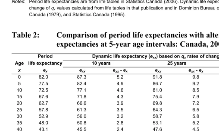
Table 2: Comparison of period life expectancies with alternative dynamic life expectancies at 5-year age intervals: Canada, 2001, females

Period Dynamic life expectancy (exx) based on qx rates of change in the previous --

Age life expectancy 10 years 25 years 50 years

x ex exx exx - ex exx exx - ex exx exx - ex

0 82.0 87.3 5.2 91.8 9.8 91.9 9.8 5 77.5 82.4 4.9 86.7 9.2 86.7 9.3 10 72.5 77.1 4.6 81.0 8.5 81.1 8.6 15 67.6 71.8 4.3 75.4 7.9 75.5 8.0 20 62.7 66.6 3.9 69.8 7.2 70.0 7.3 25 57.8 61.3 3.5 64.3 6.5 64.4 6.7 30 52.9 56.0 3.2 58.7 5.8 58.8 6.0 35 48.0 50.8 2.8 53.1 5.2 53.3 5.3 40 43.1 45.5 2.4 47.6 4.5 47.8 4.6 45 38.4 40.4 2.0 42.2 3.8 42.3 4.0 50 33.7 35.3 1.7 36.9 3.2 37.0 3.3 55 29.1 30.4 1.3 31.7 2.6 31.8 2.7 60 24.7 25.7 1.0 26.8 2.0 26.9 2.2 65 20.5 21.2 0.7 22.1 1.5 22.1 1.6 70 16.6 17.0 0.4 17.7 1.1 17.7 1.2 75 12.9 13.2 0.3 13.7 0.7 13.7 0.8 80 9.7 9.8 0.1 10.1 0.5 10.1 0.5 85 7.0 7.0 0.1 7.2 0.3 7.2 0.3 90 4.9 5.0 0.0 5.1 0.2 5.1 0.1 95 3.5 3.5 0.0 3.6 0.1 3.5 0.1 100 2.4 2.5 0.1 2.5 0.1 2.4 0.0

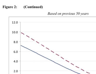
Figure 2: Number of years by which dynamic life expectancies exceed period life expectancies, Canada 2001, based on rates of change of death probabilities over the previous 10, 25, and 50 years

Based on previous 10 years

0.0 2.0 4.0 6.0 8.0 10.0 12.0

0 5 _{10 15 20 25 30 35 40 45 50 55 60 65 70 75 80 85 90 95}

10

0

Based on previous 25 years

0.0 2.0 4.0 6.0 8.0 10.0 12.0

0 5 _{10 15 20 25 30 35 40 45 50 55 60 65 70 75 80 85 90 95}

Figure 2: (Continued)

Based on previous 50 years

0.0 2.0 4.0 6.0 8.0 10.0 12.0

0 5 _{10 15 20 25 30 35 40 45 50 55 60 65 70 75 80 85 90 95}

100

M F Age

The differences between the period and dynamic expectancies vary with the choice of historical period but for children, young adults, and younger middle-aged adults the differences are substantial in all cases. At birth a newborn male child has a life expectancy of 76.9 years according to the period calculations, a female child an expectancy of 82.0 years. According to the dynamic calculations though, male life expectancy ranges from 84.1 to 87.3 years, female life expectancy from 87.3 to 91.9. By age 60 the differences have become relatively small – roughly a year or two for each sex.

The effects of the dynamic calculations are captured most prominently by the differences at birth based alternatively on rates of change of death probabilities over intervals of 10, 25, and 50 years. A 10-year interval (1991-2001) produces for males a difference of 9.0 years, a 25-year interval a difference of 10.4, and a 50-year interval a difference of 7.2. That the 50-year calculation is so much lower than the 25-year result is attributable to the fact that mortality declines were much slower between 1951 and 1976 than between 1976 and 2001. The published period life expectancy at birth for males was 70.2 in 1976. Had it been calculated using our

dynamic procedure based on the previous 25 years it would have been 73.3, a difference of 3.1 years. This contrasts with the difference of 10.4 years in 2001 (based again on the previous 25 years) but is consistent with the overall 7.2 year difference based on rates of change of death rates over the whole of the 50-year interval.

Female life expectancies at birth show another pattern in relation to the choice of interval. The 10-year interval produces an e00−e0 difference of 5.2 years whereas the

25-year and 50-year intervals produce identical results, 9.8.

We might add at this point that the variation in differences between dynamic and period life expectancies due to the choice of historical interval may be good to have on display in presenting results. Our aim in this paper, as we emphasize, is not to suggest a method of forecasting mortality probabilities and their implications but rather to show how misleading it is to assume that a period life table provides life expectancies that can be regarded as realistic. It may be desirable in practice to show not only that dynamic expectancies are invariably greater than period expectancies but that there is uncertainty about the expectancies themselves, based on the historical record.

8. Life expectancy and mortality prediction

Any calculation of life expectancy for members of a cohort who are alive at the date of the calculation requires assumptions about future death probabilities. The assumptions may be viewed as forecasts – predictions of what is likely to happen (perhaps a range of possibilities) – or they may be artificial projections, for purposes of analysis. Life expectancies derived from a period life table assume, implicitly, that the age-specific probabilities in the table will remain constant. That is clearly unrealistic, given the history of mortality rates, and is not intended to be realistic by the constructor of the table, but it does serve to bring out the implications of period table probabilities. In the same way, the dynamic life expectancies that we propose serve to bring out the implications of maintaining the rates of change of the period table probabilities.7 _They

too should not be interpreted as based on predictions. To view them as reflecting forecasts of actual probabilities would be in contradiction of how we wish them to be

viewed. As we said in the introduction to this paper (and as the title implies) we regard our proposal as simply an extension of the standard period life table.8

To emphasize further the distinction, there are various approaches that we might take if forecasting death probabilities and the attendant life expectancies were our goal. The literature provides alternatives ranging from purely judgmental forecasts (single, "high, low, medium" options, or some similar variant), to forecasts based on a parameterization of the mortality age schedule, to stochastic forecasts based on probabilities inferred from historical time series. Parameterization is often based on some form of sigmoid-type representation of the age-survival pattern; an adaptation of the logistic function is a possibility, the Weibull function, or the Gompertz function, and there are others.9 _{Stochastic forecasting was pioneered by Ronald Lee and his}

associates, and the Lee-Carter method is now well established (Lee and Carter 1992; Lee and Tuljapurkar 1994).10 _{But again, we are not concerned here with forecasting,}

merely with showing the implications for life expectancies of the maintenance of observed rates of change of death probabilities.

9. Conclusion

The dynamic extension provides an informative supplement to standard life table calculations. Without purporting to represent predictions, dynamic life expectancies draw out the implications of observed historical rates of change of death probabilities. The use of period expectancies as if they represented the future (as happens implicitly in popular usage) implies no further change in the probabilities. The use of dynamic expectancies implies continuation of observed rates of change. At the least they convey

8 _{As Keilman (2008) observes in his study of the accuracy of European population forecasts, projections,} strictly speaking, can never be wrong (aside from calculating errors): they are simply calculations of what the future population would be under a given set of assumptions, not what it is expected to be. Projections should thus be interpreted as different from forecasts. In that sense our dynamic life expectancies should be interpreted as lying in the domain of projections.

9 _{The Gompertz function, for example, can be estimated from period death rates, examined, and projected,} thus reducing some 100 age-specific mortality rates to a small set of parameters. (We note, parenthetically, that we have used the Gompertz function in this way to represent fertility schedules by a transformation of parameters that allows one to study and project, independently, total lifetime fertility, mean age of mothers at childbirth, and the interquartile range of ages at childbirth; see Denton and Spencer 1974.)

some idea as to the possible degree of understatement that may exist in the use of period expectancies.

10. Acknowledgements

References

Bongaarts, J. (2005). Long-range trends in adult mortality: Models and projection methods. Demography 42(1): 23-49. doi:10.1353/dem.2005.0003.

Bongaarts, J. (2009). Trends in senescent life expectancy. Population Studies 63(3): 203-213. doi:10.1080/00324720903165456.

Brass, W. (1971). On the scale of mortality. In: Brass, W. (ed.). Biological Aspects of Demography. London: Taylor and Francis: 69-110.

Chiang, C.L. (1984). The life table and its applications. Malabar, Florida: R.E. Krieger Publishing Company.

Coale, A. (1963). Estimates of various demographic measures through the quasi-stable age distribution. In: Emerging techniques in population research: Proceedings of a round table at the 39th Annual Conference of the Milbank Memorial Fund, September 18-19, 1962. New York: Milbank Memorial Fund: 175-193.

Coale, A. and Demeny, P. (1966). Regional model life tables and stable populations. Princeton: Princeton University Press.

Coale, A. and Demeny, P. (1967). Methods of estimating basic demographic measures from incomplete data, manuals on methods of estimating population, manual 4. New York: United Nations, Department of Economic and Social Affairs.

Denton, F.T., Feaver, C.H., and Spencer, B.G. (2005). Time series analysis and stochastic forecasting: An econometric study of mortality and life expectancy. Journal of Population Economics 18(2): 203-227. doi:10.1007/s00148-005-0229-2.

Denton, F.T. and Spencer, B.G. (1974). Some demographic consequences of changing cohort fertility patterns: An investigation using the Gompertz function. Population Studies 28(2): 309-318. doi:10.2307/2173961.

Dominion Bureau of Statistics (now Statistics Canada) (1960). Canadian life tables 1950-52 – 1955-57.Ottawa. (Catalogue 84-510).

Gompertz, B. (1825). On the nature of the function expressive of the law of mortality, and on a new mode of determining the value of life contingencies. Philosophical

Transactions of the Royal Society of London 115(24): 513-585.

Keilman, N. (2008). European demographic forecasts have not become more accurate over the past 25 years. Population and Development Review 34(1): 137-153.

doi:10.1111/j.1728-4457.2008.00209.x.

Keyfitz, N. (1968). Introduction to the mathematics of population. Reading, MA: Addison-Wesley.

Keyfitz, N. (1972). On future population. Journal of the American Statistical Association 67(338): 347-387. doi:10.2307/2284381.

Keyfitz, N. (1977). Applied mathematical demography. New York: John Wiley and Sons.

Keyfitz, N. (1982). Choice of function for mortality analysis: Effective forecasting depends on a minimum parameter representation. Theoretical Population Biology 21(3): 329-352. doi:10.1016/0040-5809(82)90022-3.

Keyfitz, N. and Caswell, H. (2005). Applied mathematical demography, 3rd _edition.

New York: Springer.

Kintner, H.J. (2004). The Life Table. In: Siegel, J.S. and Swanson, D.A. (eds.). The methods and materials of demography, 2nd _{edition. San Diego: Elsevier,}

Academic Press: 301-340. doi:10.1016/B978-012641955-9/50047-3.

Ledermann, S. (1969). Nouvelles tables-type de mortalité: Travaux et document. Paris: Institut National d'Etudes Démographiques.

Lee, R. and Tuljapurkar, S. (1994). Stochastic population forecasts for the United States: Beyond high, medium, and low. Journal of the American Statistical Association 89(428): 1175-1189. doi:10.2307/2290980.

Lee, R.D. and Carter, L.R. (1992). Modeling and forecasting U.S. mortality. Journal of the American Statistical Association 87(419): 659-671. doi:10.2307/2290201.

Makeham, W. (1860). On the law of mortality and the construction of annuity tables. Journal of the Institute of Actuaries 13: 325-358.

Murray, C.J.L., Ferguson, B.D., Lopez, A.D., Guillot, M., Salomon, J.A., and Ahmad, O. (2001). Modified logit life table system: Principles, empirical validation and application. World Health Organization. (GPE Discussion Paper; 39).

Oeppen, J. and Vaupel, J.W. (2002). Broken limits to life expectancy. Science 296(5570): 1029-1031. doi:10.1126/science.1069675.

Statistics Canada (1995). Life tables, Canada and provinces 1990-1992. Ottawa. (Catalogue 84-537).

Statistics Canada (2006). Life tables, Canada, provinces and territories 2000 to 2002. Ottawa. (Catalogue 84-537-XIE).

Suchindran, C.M. (2004). Model life tables. In: Siegel, J.S. and Swanson, D.A. (eds.). The methods and materials of demography, 2nd _{edition. San Diego: Elsevier,}

Academic Press: 662-675.

Tuljapurkar, S., Li, N., and Boe, C. (2000). A universal pattern of mortality decline in the G7 countries. Nature 405(15 June 2000): 789-792. doi:10.1038/35015561.

Appendix

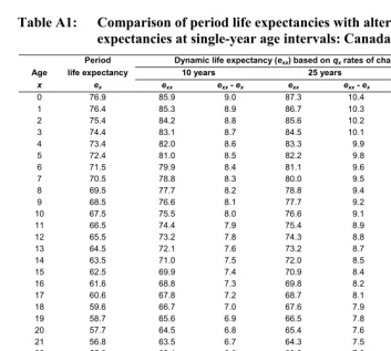
Table A1: Comparison of period life expectancies with alternative dynamic life expectancies at single-year age intervals: Canada, 2001, males

Period Dynamic life expectancy (exx) based on qx rates of change in the previous --

Age life expectancy 10 years 25 years 50 years

x ex exx exx - ex exx exx - ex exx exx - ex

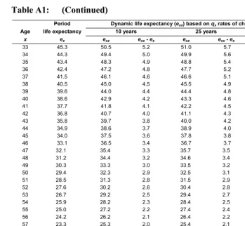
Table A1: (Continued)

Period Dynamic life expectancy (exx) based on qx rates of change in the previous --

Age life expectancy 10 years 25 years 50 years

x ex exx exx - ex exx exx - ex exx exx - ex

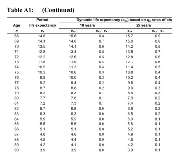
Table A1: (Continued)

Period Dynamic life expectancy (exx) based on qx rates of change in the previous --

Age life expectancy 10 years 25 years 50 years

x ex exx exx - ex exx exx - ex exx exx - ex

68 14.8 15.6 0.8 15.7 0.9 15.5 0.7 69 14.1 14.8 0.7 15.0 0.8 14.7 0.6 70 13.5 14.1 0.6 14.2 0.8 14.0 0.5 71 12.8 13.4 0.5 13.5 0.7 13.3 0.5 72 12.2 12.6 0.5 12.8 0.6 12.6 0.4 73 11.5 11.9 0.4 12.1 0.6 11.9 0.4 74 10.9 11.3 0.4 11.4 0.5 11.3 0.4 75 10.3 10.6 0.3 10.8 0.4 10.7 0.3 76 9.8 10.0 0.3 10.2 0.4 10.1 0.3 77 9.2 9.4 0.2 9.6 0.4 9.5 0.3 78 8.7 8.8 0.2 9.0 0.3 8.9 0.2 79 8.2 8.3 0.1 8.4 0.3 8.4 0.2 80 7.7 7.8 0.1 7.9 0.2 7.9 0.2 81 7.2 7.3 0.1 7.4 0.2 7.4 0.2 82 6.7 6.8 0.0 6.9 0.2 6.9 0.1 83 6.3 6.3 0.0 6.5 0.2 6.4 0.1 84 5.9 5.9 0.0 6.0 0.1 6.0 0.1 85 5.5 5.5 0.0 5.6 0.1 5.6 0.1 86 5.1 5.1 0.0 5.2 0.1 5.2 0.1 87 4.8 4.8 0.0 4.9 0.1 4.9 0.1 88 4.5 4.4 0.0 4.5 0.1 4.5 0.1 89 4.2 4.1 0.0 4.2 0.1 4.2 0.0 90 3.9 3.9 0.0 3.9 0.1 3.9 0.0 91 3.6 3.6 0.0 3.7 0.1 3.7 0.0 92 3.4 3.4 0.0 3.5 0.1 3.5 0.0 93 3.3 3.2 0.0 3.3 0.0 3.3 0.0 94 3.0 3.0 0.0 3.1 0.1 3.1 0.0 95 2.8 2.8 0.0 2.9 0.0 2.9 0.0 96 2.6 2.6 0.0 2.7 0.0 2.7 0.0 97 2.5 2.4 0.0 2.5 0.0 2.5 0.0 98 2.3 2.3 0.0 2.3 0.0 2.3 0.0 99 2.1 2.1 0.0 2.2 0.0 2.1 0.0 100 2.0 2.0 0.0 2.0 0.0 2.0 0.0

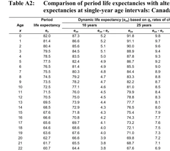
Table A2: Comparison of period life expectancies with alternative dynamic life expectancies at single-year age intervals: Canada, 2001, females

Period Dynamic life expectancy (exx) based on qx rates of change in the previous --

Age life expectancy 10 years 25 years 50 years

x ex exx exx - ex exx exx - ex exx exx - ex

Table A2: (Continued)

Period Dynamic life expectancy (exx) based on qx rates of change in the previous --

Age life expectancy 10 years 25 years 50 years

x ex exx exx - ex exx exx - ex exx exx - ex

Table A2: (Continued)

Period Dynamic life expectancy (exx) based on qx rates of change in the previous --

Age life expectancy 10 years 25 years 50 years

x ex exx exx - ex exx exx - ex exx exx - ex

68 18.1 18.7 0.5 19.4 1.3 19.4 1.3 69 17.3 17.8 0.5 18.5 1.2 18.6 1.2 70 16.6 17.0 0.4 17.7 1.1 17.7 1.2 71 15.8 16.2 0.4 16.8 1.0 16.9 1.1 72 15.1 15.4 0.4 16.0 0.9 16.1 1.0 73 14.3 14.7 0.3 15.2 0.9 15.3 0.9 74 13.6 13.9 0.3 14.4 0.8 14.5 0.8 75 12.9 13.2 0.3 13.7 0.7 13.7 0.8 76 12.2 12.5 0.2 12.9 0.7 12.9 0.7 77 11.6 11.8 0.2 12.2 0.6 12.2 0.6 78 10.9 11.1 0.2 11.5 0.6 11.5 0.6 79 10.3 10.4 0.1 10.8 0.5 10.8 0.5 80 9.7 9.8 0.1 10.1 0.5 10.1 0.5 81 9.1 9.2 0.1 9.5 0.4 9.5 0.4 82 8.5 8.6 0.1 8.9 0.4 8.9 0.4 83 8.0 8.0 0.1 8.3 0.3 8.3 0.3 84 7.4 7.5 0.1 7.8 0.3 7.7 0.3 85 7.0 7.0 0.1 7.2 0.3 7.2 0.3 86 6.5 6.6 0.1 6.7 0.2 6.7 0.2 87 6.1 6.1 0.1 6.3 0.2 6.3 0.2 88 5.7 5.7 0.1 5.9 0.2 5.8 0.2 89 5.3 5.4 0.1 5.5 0.2 5.4 0.2 90 4.9 5.0 0.0 5.1 0.2 5.1 0.1 91 4.6 4.7 0.0 4.8 0.1 4.7 0.1 92 4.3 4.4 0.0 4.4 0.1 4.4 0.1 93 4.0 4.0 0.0 4.1 0.1 4.1 0.1 94 3.7 3.8 0.0 3.8 0.1 3.8 0.1 95 3.5 3.5 0.0 3.6 0.1 3.5 0.1 96 3.2 3.3 0.0 3.3 0.1 3.3 0.1 97 3.0 3.0 0.0 3.1 0.1 3.0 0.0 98 2.8 2.8 0.1 2.9 0.1 2.8 0.0 99 2.6 2.6 0.0 2.7 0.1 2.6 0.0 100 2.4 2.5 0.1 2.5 0.1 2.4 0.0