Approximate solution of a system of singular integral equations of the first kind by using Chebyshev polynomials

Galley

Pro

of

Vol. 9, No. 2, (2019), pp 31–47 DOI:10.22067/ijnao.v9i2.73724

————————————————————————————————————

Research Article

Approximate solution of a system of

singular integral equations of the first

kind by using Chebyshev polynomials

S. Ahdiaghdam∗ and S. Shahmorad

Abstract

The aim of the present work is to introduce a method based on the Cheby-shev polynomials for numerical solution of a system of Cauchy type singular integral equations of the first kind on a finite segment. Moreover, an esti-mation error is computed for the approximate solution. Numerical results demonstrate the effectiveness of the proposed method.

AMS(2010): 45F15; 33C45; 42C10; 41A50.

Keywords: System of singular linear integral equations; Orthogonal poly-nomials; Fourier series; Best approximation.

1 Introduction

Let us consider a system of singular integral equations of the form

A(t)Φ(t) +B(t) ∫ 1

−1

Φ(τ)

τ−tdτ+

∫ 1

−1

K(t, τ)Φ(τ)dτ =F(t), −1< t <1,(1)

where

∗_{Corresponding author}

Received 25 June 2018; revised 7 December 2018; accepted 23 January 2019 Samad Ahdiaghdam

Department of Mathematics, Marand Branch, Islamic Azad University, Marand, Iran. e-mail: [email protected]

Sedaghat Shahmorad

Department of Applied Mathematics, University of Tabriz, Tabriz, Iran. e-mail: [email protected]

Galley

Pro

of

K(t, τ) = [Kij(t, τ)], i, j= 1,2, . . . , N,

F(t) = [f1(t), f2(t), . . . , fN(t)]T,

Φ(t) = [ϕ1(t), ϕ2(t), . . . , ϕN(t)]T,

A(t) = [aij(t)], i, j= 1,2, . . . , N,

B(t) = [bij(t)], i, j= 1,2, . . . , N.

Here, {Kij}Ni,j=1 and {fi}Ni=1 are given real-valued H¨older functions and

{ϕj}Nj=1 are the unknown functions. The matricesAandB are known such

that S=A+B andD =A−B are nonsingular for allt∈[−1,1]. In some familiar physical problems, the entries of the matricesAandBare constants. The singular integral equations play important roles in physics and the-oretical mechanics, particularly in the areas of elasticity, aerodynamics, and unsteady aerofoil theory. They are highly effective in solving boundary value problems occurring in the theory of functions of a complex variable, potential theory, the theory of elasticity, and the theory of fluid mechanics. A general theory of the system of equations (1) has given in [12].

We study the system (1) in the case thatA(t) = 0 andB(t) is a constant matrix. Therefore, theith equation of system (1) takes the form

N

∑

j=1

bij

∫ 1

−1

ϕj(τ)

τ−t dτ+

N

∑

j=1

∫ 1

−1

Kij(t, τ)ϕj(τ)dτ =fi(t), −1< t <1. (2)

Studies on this singular integral equation can be found in some literatures (see [1,3,6,7]). Chakrabarti and Berghe [3] proposed a method for solving (2), using polynomial approximation and collocation points have chosen to be the zeros of the Chebyshev polynomials of the first kind for all cases. Kashfi and Shahmorad [7] constructed another approximate solution of this equation by using the Chebyshev polynomials of the first and second kinds. Some other methods for solving this equation can be found in [1,6]. A convergence analysis of Galerkin and collocation methods for (2) has been given by Miel [11].

A special type of (2) is the famous Cauchy singular integral equation ∫ 1

−1

ϕ(τ)

τ−tdτ =f(t), −1< t <1, (3)

which has the following analytical solutions in four special cases based on boundedness of the unknown function ϕ at the endpoints of the interval [−1, 1]; see [3,9,13].

Case 1. If the function ϕis unbounded at the endpoints τ=±1, then

ϕ(τ) =√ a0 1−τ2 −

1

π2√₁−_τ2

∫ 1

−1

√

1−t2_f(t)

Galley

Pro

of

Case 2. If the function ϕis bounded at the endpoints τ=±1, then

ϕ(τ) =− √

1−τ2

π2

∫ 1

−1

f(t) √

1−t2_(t−τ)dt , −1< τ <1,

and a necessary and sufficient condition of existing this solution is ∫ 1

−1

f(t) √

1−t2dt= 0.

Case 3. If the functionϕis bounded at the endpointτ =−1 and unbounded at the endpointτ = 1, then

ϕ(τ) =− 1

π2

√ 1 +τ

1−τ

∫ 1

−1

√ 1−t

1 +t f(t)

t−τdt , −1< τ <1.

Case 4. If the functionϕis bounded at the endpointτ= 1 and unbounded at the endpointτ =−1, then

ϕ(τ) =− 1

π2

√ 1−τ

1 +τ

∫ 1

−1

√ 1 +t

1−t f(t)

t−τdt , −1< τ <1.

An application of (3) were given in [2] by reducing a system of dual integral equations to Cauchy type singular integral equations, and more methods for solving this equation have given in [5,8,13,15].

In the next section, we investigate approximate solutions for system (1) in the above four cases.

2 Approximate solution

To find approximate solutions for system (1) in the cases 1,2,3,4, for ν ∈

{1,2,3,4}, we set

ϕj(τ)≃φν,j(τ) :=

λν(τ)

√ 1−τ2

M

∑

l=0

βjlPν,l(τ), j= 1,2, . . . , N, (4)

Galley

Pro

of

Kij(t, τ) := M

∑

k=0

γijk(t)Pν,k(τ), i, j= 1,2, . . . , N , (5)

where

Pν,j(x) =

                        

Tj(x) = cos(jθ), ν = 1,

Uj(x) =

sin((j+1)θ)

sin(θ) , ν = 2,

Vj(x) =

cos((j+1 2)θ)

cos(θ

2)

, ν = 3,

Wj(x) =

sin((j+1 2)θ)

sin(θ

2)

, ν = 4,

are the Chebyshev polynomials of the first to fourth kinds and

λν(t) =

      

1, ν = 1,

1−t2_{, ν = 2,}

1 +t, ν = 3,

1−t, ν = 4,

in which x = cos(θ). The roots of Chebyshev polynomials Pν,M+1(x) are

given by

xν,n=

                           cos (

(2n−1)π

2(M+1)

)

, ν= 1,

cos (

nπ M+2

)

, ν= 2,

cos (

(2n−1)π

2M+3

)

, ν= 3,

cos (

2nπ

2M+3

)

, ν= 4,

(6)

where n = 1,2, . . . , M + 1. These roots are used as the nodes of Gauss– Chebyshev quadrature rules.

Galley

Pro

of

−1

λν(t)

√

1−t2Pν,i(t)Pν,j(t)dt =

                          

0, i̸=j,

π, i=j= 0, ν = 1,

π

2, i=j̸= 0, ν= 1,

π

2, i=j, ν = 2,

π, i=j, ν = 3,4.

(7)

Theorem 1. [10] As the Cauchy principle value of a singular integral, we have

∫ 1

−1

λν(τ)

√ 1−τ2

Pν,j(τ)

τ−t dτ =π

                  

Uj−1(t), ν= 1,

−Tj+1(t), ν= 2,

Wj(t), ν= 3,

−Vj(t), ν= 4.

(8)

Now we describe details of finding approximate solution in cases1-4.

Case 1. Forν = 1, the relations (4)–(5) take the forms

ϕj(τ)≃φ1,j(τ) :=

1 √

1−τ2

M

∑

l=0

′

βjlTl(τ), j = 1,2, . . . , N, (9)

and

Kij(t, τ) := M

∑

k=0

′

γijk(t)Tk(τ), i, j= 1,2, . . . , N, (10)

where βjl (j = 1,2, . . . , N, l = 0,1, . . . , M) are unknown coefficients and

the symbol (∑′) denotes that the first term in the summation is halved. The functions

γijk(t) =

2

π

∫ 1

−1

Kij_√(t, τ)Tk(τ)

1−τ2 dτ , i, j= 1,2, . . . , N, k= 0,1, . . . , M,

can be determined exactly or may be approximated by using the Gauss– Chebyshev quadrature rule, that is,

γijk(t)≃

2

M+ 1

M_∑+1

s=1

Kij(t, x1,s)Tk(x1,s),

Galley

Pro

of

bijβjlUl₋1(t) +

1 2 N ∑ j=1 M ∑ k=0 ′

γijk(t)βjk=

1

πfi(t), i= 1,2, . . . , N.(11)

If the given functionsfi and γijk are square integrable on [−1, 1] with

respect to the weight function _√λ1(t)

1₋t2, then they can be expanded as

  

γijk(t)≃

∑M₋1

l=0 GijklUl(t), i, j= 1,2, . . . , N, k= 0,1, . . . , M,

1

πfi(t)≃

∑M₋1

l=0 cilUl(t), i= 1,2, . . . , N,

(12)

where the coefficients               

Gijkl =_π2

∫1

−1

√ 1−t2_γ

ijk(t)Ul(t)dt

=_π42

∫1

−1

∫1

−1

√

1−t2

1−τ2Kij(t, τ)Ul(t)Tk(τ)dτ dt

i, j= 1,2, . . . , N, k= 0,1, . . . , M, l= 0,1, . . . , M−1,

cil =_π12

∫1

−1

√ 1−t2_f

i(t)Ul(t)dt, i= 1,2, . . . , N, l= 0,1, . . . , M−1,

can be approximately determined from 

   

Gijkl≃ _(M+1)4 2

∑M r=1

∑M+1

s=1 (1−x 2

2,r)Kij(x2,r, x1,s)Ul(x2,r)Tk(x1,s),

cil≃_π(M2₊₁₎

∑M

r=1(1−x 2

2,r)fi(x2,r)Ul(x2,r).

(13)

Using (12) in (11), we have

M_∑−1

l=0

N

∑

j=1

bijβj{l+1}Ul(t) +

1 2

M_∑−1

l=0 N ∑ j=1 M ∑ k=0 ′

GijklβjkUl(t) = M_∑−1

l=0

cilUl(t),

which leads to the linear system

N

∑

j=1

[

bijβj_{l+1_}+

1 2 M ∑ k=0 ′

Gijklβjk

]

=cil, i= 1,2, . . . , N, l= 0,1, . . . , M−1,

(14)

for the unknown values βjk (j = 1,2, . . . , N, k = 0,1, . . . , M).

Tak-ingβ11, . . . , βN1arbitrary, the remaining coefficientsβjk are uniquely found

Galley

Pro

of

− N ∑ j=1 M ∑ l=0

bijβjlTl+1(t) +

1 2 N ∑ j=1 M ∑ k=0

γijk(t)βjk=

1

πfi(t), i= 1,2, . . . , N,(15)

where we used the formulas (7)–(8). Then, we expand the functions fi and

γijk as

  

γijk(t)≃

∑M l=0

′

GijklTl(t), i, j= 1,2, . . . , N, k= 0,1, . . . , M

1

πfi(t)≃

∑M l=0

′

cilTl(t), i= 1,2, . . . , N,

where the coefficients are determined by           

Gijkl =_π2

∫1

−1 1

√

1−t2γijk(t)Tl(t)dt, i, j= 1,2, . . . , N, k, l= 0,1, . . . , M,

=_π42

∫1

−1

∫1

−1

√

1₋τ2

1₋t2Kij(t, τ)Tl(t)Uk(τ)dτ dt

cil= _π22

∫1

−1 1

√

1−t2fi(t)Tl(t)dt, i= 1,2, . . . , N, l= 0,1, . . . , M,

or approximated by 

   

Gijkl ≃_(M+1)(4_M+2)

∑M+1

r=1

∑M+1

s=1 (1−x 2

2,s)Kij(x1,r, x2,s)Tl(x1,r)Uk(x2,s),

cil≃ _π(M2₊₁₎

∑M+1

r=1 fi(x1,r)Tl(x1,r).

Using the last expansions in (15), returns the following linear system of equa-tions      1 2 ∑N j=1 ∑M

k=0Gijklβjk=cil, i= 1, . . . , N, l= 0,

∑N j=1

{

−bijβj{l−1}+12

∑M

k=0Gijklβjk

}

=cil, i= 1, . . . , N, l= 1, . . . , M,

for the unknown values βjl (j = 1,2, . . . , N, l = 0,1, . . . , M). Then

ele-ments of the vector function Φ(t) obtain from (4).

Cases 3,4. Similar to cases 1 and 2, we get the linear systems

N

∑

j=1

{

bijβjl+ M

∑

k=0

Gijklβjk

}

=cil, i= 1,2, . . . , N, l= 0,1, . . . , M, (16)

Galley

Pro

of

N

∑

j=1

{

−bijβjl+ M

∑

k=0

Gijklβjk

}

=cil, i= 1,2, . . . , N, l= 0,1, . . . , M,(17)

respectively for ν = 3 and ν = 4, and then we determine the elements of corresponding vector Φ via (4).

3 An estimation error and numerical results

In this section, we describe an estimation error for the approximate solution. Let

Φ(t) = [φ1(t), φ2(t), . . . , φN(t)]T

be the vector of approximate solution of the system (1) and letE(t) = Φ(t)− Φ(t) be the associated vector valued error function. Due to the approximation Φ(t), forA(t) = 0, system (1) may be written as

B(t) ∫ 1

−1

Φ(τ)

τ−tdτ +

∫ 1

−1

K(t, τ)Φ(τ)dτ =F(t) +H(t), −1< t <1, (18)

where the perturbation term H(t) obtains from

H(t) =B(t) ∫ 1

−1

Φ(τ)

τ−tdτ+

∫ 1

−1

K(t, τ)Φ(τ)dτ −F(t), −1< t <1.

Subtracting (18) from (1) yields a system of error equations as

B(t) ∫ 1

−1

E(τ)

τ−tdτ+

∫ 1

−1

K(t, τ)E(τ)dτ =H(t), −1< t <1,

which is solvable approximately like system (1).

The following examples illustrate application of the method.

Example 1. Let

A(t) = 0, B(t) = [

1 0 0 1 ]

, K(t, τ) = [

τ−t t τ τ+t

]

, F(t) = [

π

2πt

]

,

and find the solution of system (1) in case1.

By the above information, the system (1) is reduced to 

   

∫1

−1

ϕ1(τ)

τ₋t dτ +

∫1

−1(τ−t)ϕ1(τ)dτ+

∫1

−1tϕ2(τ)dτ =π, −1< t <1,

∫1

−1

ϕ2(τ)

τ−t dτ +

∫1

−1τ ϕ1(τ)dτ+

∫1

−1(τ+t)ϕ2(τ)dτ = 2πt,−1< t <1,

Galley

Pro

of

then system (19) has a unique solution. The kernels K1j(t, τ), K2j(t, τ)

(j= 1,2), and the functionsf1 andf2 are polynomials of degree at most 1,

so we set

ϕj(τ) :=

1 √

1−τ2{βj0T0(τ) +βj1T1(τ) +βj2T2(τ)}, j= 1,2, (20)

and

Kij(t, τ) =γij0(t)T0(τ) +γij1(t)T1(τ), i, j= 1,2,

fi(t) =ci0U0(t) +ci1U1(t), i= 1,2,

where

γ110(t) =−1₂U1(t), γ111(t) =U0(t), γ120(t) = 1₂U1(t), γ121(t) = 0,

γ210(t) = 0, γ211(t) =U0(t), γ220(t) = 1₂U1(t), γ221(t) =U0(t),

c10(t) = 1, c11(t) = 0, c20(t) = 0, c21(t) = 1.

Substituting these expansions into (19) and using (7)–(8), for ν = 1, we obtain

  

β11U0(t) +β12U1(t)−1₂β10U1(t) +1₂β11U0(t) +1₂β20U1(t) =U0(t),

β21U0(t) +β22U1(t) +12β11U0(t) +12β20U1(t) +12β21U0(t) =U1(t).

Then the linear independency of{U0(t), U1(t)} implies

      

3

2β11= 1,

−1

2β10+β12+ 1

2β20= 0, 1

2β11+ 3

2β21= 0, 1

2β20+β22= 1.

A nonunique solution of this system for the arbitrary values ofβ10 and β20

is given by

β10, β11=

2

3, β12= 1

2(β10−β20), β20, β21=− 2

9, β22= 1− 1 2β20. For example, ifβ10=β20 = 2, thenβ12 =β22= 0 and so we find from (20)

that

ϕ1(τ) = 2 3τ+ 2

√

1−τ2, ϕ2(τ) =

−2 9τ+ 2

√ 1−τ2 ,

(see Figure1 for the behavior of these solutions).

Galley

Pro

of

ϕj(τ) :=

√ 1 +τ

1−τ {βj0V0(τ) +βj1V1(τ)} , j = 1,2, (21)

and

Kij(t, τ) =γij0(t)V0(τ) +γij1(t)V1(τ), i, j= 1,2,

fi(t) =ci0W0(t) +ci1W1(t), i= 1,2,

where

γ110(t) =W0(t)−1₂W1(t), γ111(t) =γ210(t) =γ211(t) =γ221(t) = 1₂W0(t),

γ120(t) =−1₂W0(t) +1₂W1(t), γ121(t) = 0, γ220(t) =1₂W1(t),

c10(t) = 1, c11(t) = 0, c20(t) =−1, c21(t) = 1.

Substituting these expansions into (19) and using (7)–(8) forν= 3, result 

         

β10W0(t) +β11W1(t) +β10W0(t)−1₂β10W1(t)

+1₂β11W0(t)−1₂β20W0(t) +1₂β20W1(t) =W0(t),

β20W0(t) +β21W1(t) +1₂β10W0(t) +1₂β11W0(t)

+1

2β20W1(t) + 1

2β21W0(t) =−W0(t) +W1(t),

and from the linear independency of{W0(t) andW1(t)}, we get the algebraic

system

      

2β10+1₂β11−1₂β20= 1,

−1

2β10+β11+ 1

2β20= 0, 1

2β10+ 1

2β11+β20+ 1

2β21=−1, 1

2β20+β21= 1,

Galley

Pro

of

β10=−

10

27, β11= 28

27, β20=− 22

9 , β21= 20

9 ,

and the solutions of (19) can be found via (21). The graphs of these solutions plotted in Figure2.

Example 3. Solve the following system in the case3[16]: 

   

3∫₋1₁ϕ1(τ)

τ−t dτ +

∫1

−1

ϕ2(τ)

τ−t dτ = (t

2_{+ 1) sin 2t,−1< t <1,}

2∫₋1₁ϕ1(τ)

τ−t dτ +

∫1

−1

ϕ2(τ)

τ−t dτ =tcos 2t, −1< t <1.

In this case, we will approximate the unknown functions as

ϕi(τ)≃φi(τ) :=

√ 1−τ2

M

∑

j=0

βijUj(τ), i= 1,2,

where the exact solutions are 

     

ϕ1(τ) =−

√

1₋τ2

π2

∫1

−1

(t2_{+1) sin 2t−tcos 2t} √

1−t2_(t−τ) dt, ϕ2(τ) =−

√

1₋τ2

π2

∫1

−1

3tcos 2t−2(t2_{+1) sin 2t} √

1−t2_(t−τ) dt.

We define the error functions as

Ei(τ) =|ϕi(τ)−φi(τ)|, i= 1,2,

where the exact solutionsϕ1 andϕ2are calculated by using the Maple code

Galley

Pro

of

τ ϕ1(τ) ϕ2(τ) E1(τ) E2(τ) ε1(τ) ε2(τ) −0.96 −0.2164694659571311 0.5107921932649533 1e−8 2e−8 8e−5 2e−4

−0.70 −0.5394637532569845 1.185306580331174 3e−7 6e−7 4e−5 1e−4

−0.25 ₋0.5831756914063946 1.129312022840245 4e₋7 9e₋7 9e₋6 2e₋5 0.25 ₋0.5831756914063946 1.129312022840245 4e₋7 9e₋7 9e₋6 2e₋5 0.75 ₋0.5394637532569845 1.185306580331174 3e₋7 6e₋7 4e₋5 1e₋4 0.96 ₋0.2164694659571311 0.5107921932649533 1e₋8 2e₋8 8e₋5 2e₋4

Table 2: The approximated valuesφi(τ) forM= 15 by using 16-digits arithmetic.

τ φ1(τ) φ2(τ) E1(τ) E2(τ) ε1(τ) ε2(τ) −0.96 −0.2164694659571311 0.5107921932649527 0 6e−16 -

-−0.70 −0.5394637532569844 1.185306580331173 1e−16 1e−15 -

-−0.25 −0.5831756914063935 1.129312022840244 1e−15 1e−15 - -0.25 −0.5831756914063935 1.129312022840244 1e−15 1e−15 - -0.75 −0.5394637532569844 1.185306580331173 1e−16 1e−15 - -0.96 −0.2164694659571311 0.5107921932649527 0 6e−16 -

-In Table1, we compared our numerical results (absolute errors E1 and

E2) with those reported in [16] (absolute errors ε1 and ε2). Table 2 shows

our results forM = 15, which were not reported in [16].

Example 4. Consider the singular integral equation ∫ 1

−1

ϕ(τ)

τ−tdτ +

∫ 1

−1

eitϕ(τ)dτ = 1−2t2+it+1 2e

−it_{, −1< t <1, (22)}

with the exact solution ϕ(τ) = √1_π−τ2(2τ−i) in the complex plane, where i=√−1.

By takingϕ1:=Re{ϕ}andϕ2:=Im{ϕ}, equation (22) is reduced to the

system of singular integral equations 

 

∫1

−1 ϕ1(τ)

τ−t dτ+

∫1

−1cos(t)ϕ1(τ)dτ−

∫1

−1sin(t)ϕ2(τ)dτ = 1−2t 2₊1

2sint,−1< t <1,

∫1

−1 ϕ2(τ)

τ−t dτ+

∫1

−1sin(t)ϕ1(τ)dτ+

∫1

−1cos(t)ϕ2(τ)dτ =t− 1

2cost, −1< t <1.

Similar to Examples 1 and 2, by setting

ϕi(τ)≃φi(τ) :=

√ 1−τ2

M

∑

j=0

βijUj(τ), i= 1,2,

we get the exact solutions for M = 1.

Galley

Pro

of

ϕ1(τ)

τ−t dτ+

10

π

∫1

−1

ϕ2(τ)

τ−t dτ =f1(t) +ig1(t),−1< t <1,

500

π

∫1

−1

ϕ1(τ)

τ₋t dτ+

200

π

∫1

−1

ϕ2(τ)

τ₋t dτ =f2(t) +ig2(t),−1< t <1,

(23) where         

f1(t) =−990t8+ 1089t7+ 937t6−2670425 t

5₋349161 1000 t

4₊792327 2000 t

3₊1761 250t

2₋53511 4000t−

53929 2000,

g1(t) = 990t8−1189t7−897110 t

6₊119047 100 t

5₊163961 500 t

4₋279198 625 t

3₋30873 10000t

2₊69533

4000t+113050140000 ,

f2(t) =−300t8+ 330t7+ 215t6−244710 t 5₋8607

100t 4₊735

8 t 3₋17253

2000t 2₊29541

4000t−147011000,

g2(t) = 300t8−380t7−197t6+14625 t 5₊9419

100t 4₋27549

250 t 3₋183

400t 2₋7957

2000t+575834000.

It is easy to see that system (23) is equivalent to the following disjointed singular integral equations,

                         1 π ∫1 −1

Re{ϕ1(τ)}

τ₋t dτ =

20f1(t)−f2(t)

19500 , −1< t <1, 1

π

∫1

−1

Im{ϕ1(τ)}

τ−t dτ =

20g1(t)−g2(t)

19500 ,−1< t <1, 1

π

∫1

−1

Re_{ϕ2(τ)}

τ−t dτ =

2f2(t)−f1(t)

390 , −1< t <1, 1

π

∫1

−1

Im{ϕ2(τ)}

τ₋t dτ =

2g2(t)−g1(t)

390 , −1< t <1.

(24)

The exact solution of system (23) was reported in [14] for the case r = 4. By applying our method for the equation in (24), we get the real parts of unknown functions exactly but, for the imaginary parts, we obtain the error functions

Ei(τ) =|Im{ϕi(τ)} −Im{φi(τ)}|=

√ 1−τ

1 +τhi(τ), i= 1,2,

where {

h1(τ) = 5.128205128205128×10−8(1 +τ), −1< τ <1,

h2(τ) = 5.128205128205128×10−6(1 +τ), −1< τ <1.

The plots of h1 and h2 and the regular parts of the error functions, are

shown in Figure 3. As shown in these plots, the absolute errors increase when τ approaches to 1, because in case 4, the singularity for the integral part happens atτ = 1.

Galley

Pro

of

      

∫1

−1

ϕ1(τ)

τ−t dτ+

∫1

−1[K11(t, τ)ϕ1(τ) +K12(t, τ)ϕ2(τ)dτ] = 0,

∫1

−1

ϕ2(τ)

τ₋t dτ+

∫1

−1

[

K21(t, τ)ϕ1(τ) +K22(t, τ)ϕ2(τ)dτ

] =π,

(25)

with

K11(t, τ) =−_(τ−tτ₎−2₊₄t _h2 +

8h2(τ−t) [(τ₋t)2_+4h2_]2 −

4h2(τ−t)[12h2−(τ−t)2]

[(τ₋t)2_+4h2_]3 , K12(t, τ) =K21(t, τ) =−

8h3[4h2−3(τ−t)2]

[(τ−t)2_+4h2_]3 , K22(t, τ) =−_(τ−tτ₎−2₊₄t _h2 −

8h2_(τ−t)

[(τ−t)2_+4h2_]2 −

4h2_(τ−t)[12h2_−(τ−t)2_]

[(τ−t)2_+4h2_]3 ,

wherehis the distance of crack from the boundary. The physical conditions of the problem impose that the relations

∫ 1

−1

ϕ1(τ)dτ = 0,

∫ 1

−1

ϕ2(τ)dτ = 0, (26)

and

ϕ1(t) =ϕ1(−t), ϕ2(t) =−ϕ2(−t)

are satisfied. Therefore the unknown functions may be expressed as

ϕ1(τ)≃

1 √

1−τ2

M

∑

j=0

β1jT2j(τ), ϕ2(τ)≃

1 √

1−τ2

M

∑

j=1

Galley

Pro

of

Forν= 1, it follows from the orthogonality condition (7) that the second condition in (26) satisfies and the first one givesβ10= 0.

Takingβ11 =β21 = 0, the remaining coefficientsβij are uniquely

deter-mined from the linear algebraic system (14) for each values ofhandM.This leads to find the functionsϕ1and ϕ2 from (27).

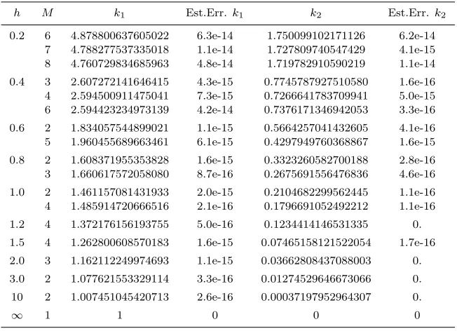
The stress intensity factors

k1= lim

τ_→1−

√

1−τ2_ϕ 2(τ)

k2= lim

τ→1−

√

1−τ2_ϕ 1(τ)

and their absolute estimation errors(Est.Err.) are reported in Table 3. For

h=∞andKij(t, τ) = 0,from (27) and (13)–(14), the exact solutions of (25)

are obtained as

ϕ1(τ) = 0, ϕ2(τ) =

τ

√ 1−τ2,

which give k1 = 1 and k2 = 0. This is shown in the last row of Table 3.

The table shows the rapid convergence of the results even for relatively small values ofM.

4 Conclusions

Galley

Pro

of

h M k1 Est.Err. k1 k2 Est.Err. k2

0.2 6 4.878800637605022 6.3e-14 1.750099102171126 6.2e-14 7 4.788277537335018 1.1e-14 1.727809740547429 4.1e-15 8 4.760729834685963 4.8e-14 1.719782910590219 1.1e-14 0.4 3 2.607272141646415 4.3e-15 0.7745787927510580 1.6e-16 4 2.594500911475041 7.3e-15 0.7266641783709941 5.0e-15 6 2.594423234973139 4.2e-14 0.7376171346942053 3.3e-16 0.6 2 1.834057544899021 1.1e-15 0.5664257041432605 4.1e-16 5 1.960455689663461 6.1e-15 0.4297949760368867 1.6e-15 0.8 2 1.608371955353828 1.6e-15 0.3323260582700188 2.8e-16 3 1.660617572058080 8.7e-16 0.2675691556476836 4.6e-16 1.0 2 1.461157081431933 2.0e-15 0.2104682299562445 1.1e-16 4 1.485914720666516 2.1e-16 0.1796691052492212 1.1e-16 1.2 4 1.372176156193755 5.0e-16 0.1234414146531335 0. 1.5 4 1.262800608570183 1.6e-15 0.07465158121522054 1.7e-16 2.0 3 1.162112249974693 1.1e-15 0.03662808437088003 0. 3.0 2 1.077621553329114 3.3e-16 0.01274529646673066 0. 10 2 1.007451045420713 2.6e-16 0.00037197952964307 0.

∞ 1 1 0 0 0

References

1. Abdolkawi, M. Solution of Cauchy type singular integral equations of the first kind by using differential transform method, Appl. Math, Model. 39 (2015), 2107–2118.

2. Ahdiaghdam, S., Shahmorad S. and Ivaz, K.Approximate solution of dual integral equations using Chebyshev polynomials, Int. J. Comput. Math. 94(3) (2017), 493–502.

3. Chakrabarti, A. and Berghe, G.V.Approximate solution of singular inte-gral equations, Appl. Math. Lett., 17 (2004), 533–559.

4. Erdogan, F., Gupta, G.D. and Cook, T.S.Mechanics of fracture, Noord-hoff International Publishing, Leyden, Netherlands, 1973.

5. Eshkuvatov, Z.K., Nik Long, N.M.A. and Abdulkawi, M. Approximate solution of singular integral equations of the first kind with Cauchy kernel, Appl. Math. Lett., 22 (2009), 651–657.

Galley

Pro

of

8. Liu, D., Zhang, X. and Wu, J.A collocation scheme for a certain Cauchy singular integral equation based on the superconvergence analysis, Appl. Math. Comput. 219 (2013), 5198–5209.

9. Mandal, B.N. and Chakrabarti, A. Applied singular integral equations, Taylor and Francis Group, CRC Press, 2011.

10. Mason, J.C. and Handscomb, D.C. Chebyshev polynomials, Chapman and Hall, CRC Press, 2003.

11. Miel, G.On the Galerkin and collocation methods for a Cauchy singular integral equation, SIAM J. Numer. Anal. 23(1) (1986), 135–143.

12. Muskhelishvili, N.I. and RADOK, J.R.M. Singular integral equations, Wolters-Noordhoff Publishing Groningen, Netherlands, 1958.

13. Setia, A. Numerical solution of various cases of Cauchy type singular integral equation, Appl. Math. Comput. 230 (2014), 200–207.

14. Sharma, V., Setia, A. and Agarwal, R.Numerical solution for system of Cauchy type singular integral equations with its error analysis in complex plane, Appl. Math. Comput., 328 (2018), 338–352.

15. Tsalamengas, J.L.A direct method to quadrature rules for a certain class of singular integrals with logarithmic, Cauchy, or Hadamard-type singu-larities, Int. J. Numer. Model. 25 (2012), 512–524.