Object Detection and Tracking Using Uncalibrated Cameras

University of New Orleans University of New Orleans

ScholarWorks@UNO

ScholarWorks@UNO

University of New Orleans Theses and

Dissertations Dissertations and Theses

5-14-2010

Object Detection and Tracking Using Uncalibrated Cameras

Object Detection and Tracking Using Uncalibrated Cameras

Ashwini Amara

University of New Orleans

Follow this and additional works at: https://scholarworks.uno.edu/td

Recommended Citation Recommended Citation

Amara, Ashwini, "Object Detection and Tracking Using Uncalibrated Cameras" (2010). University of New Orleans Theses and Dissertations. 1184.

https://scholarworks.uno.edu/td/1184

This Thesis is protected by copyright and/or related rights. It has been brought to you by ScholarWorks@UNO with permission from the rights-holder(s). You are free to use this Thesis in any way that is permitted by the copyright and related rights legislation that applies to your use. For other uses you need to obtain permission from the rights-holder(s) directly, unless additional rights are indicated by a Creative Commons license in the record and/or on the work itself.

Object Detection and Tracking Using Uncalibrated Cameras

A Thesis

Submitted to the Graduate Faculty of the University of New Orleans In partial fulfillment of the Requirements for the degree of

Master of Science in

Electrical Engineering

by

Ashwini Amara

B.E. Osmania University, 2007

ii

Acknowledgements

I would like to express my deepest gratitude to my major advisor, Dr. X. Rong Li, for his invaluable inspiration, continuous support, and constructive suggestions, which made it possible for me to complete my M.S. degree. I am also indebted to Dr. Huimin Chen for his help, motivation and encouragement which made my research experience more rewarding and enjoyable. I would take this opportunity to thank Dr. Vesselin P. Jilkov for his advice, support and guidance.

I am also extending my gratefulness to all the students at Information and Systems Laboratory for providing their technical expertise in my research. I feel that I was at an advantage of having a conducive and productive work environment. Furthermore, I would like to thank all the members and staff of the Department of Electrical Engineering at the University of New Orleans for their support.

iii

Table of Contents

Table of Contents ... iii

Table of Figures ... v

Abstract ... vi

Chapter 1 Introduction ... 1

1.1 Introduction to object detection and tracking ... 1

1.2 Outline of thesis ... 4

Chapter 2 Feature Detection ... 7

2.1 Harris corner detector ... 9

2.2 Performance requirements... 12

2.3 Experiment results ... 13

2.4 Conclusions ... 15

Chapter 3 2D and 3D Vision Formation ... 16

3.1 Simple camera system-pinhole model... 16

3.1.1 External parameters ... 18

3.1.2 Rotation matrix ... 19

3.1.3 Rotation matrix representation using Euler angles ... 20

3.1.4 Intrinsic parameters ... 21

Chapter 4 Feature Matching... 23

Chapter 5 Stereo Vision ... 25

5.1 Epipolar geometry ... 25

5.1.1 Essential matrix estimation ... 28

Chapter 6 Calibration Methods ... 31

6.1 Calibration with a rig... 31

6.2 Self calibration ... 32

6.2.1 Uncalibrated epipolar geometry ... 33

6.2.2 Properties of fundamental matrix ... 34

6.3 Camera calibration using nonlinear least squares ... 35

iv

6.5 Conclusion ... 39

Chapter 7 Object Tracking Model ... 41

7.1 Nearly Constant velocity model ... 41

7.2 Measurement model ... 42

7.3 Iterative Extended Kalman filter estimation ... 43

7.4 Credibility of the filter... 44

Chapter 8 Tracking Moving Object on Synthetic Data ... 46

8.1 Generation of synthetic data ... 46

8.2 Procedure to estimate camera parameters and state vector of the object ... 47

8.3 Conclusion ... 54

Chapter 9 Conclusions and Future work ... 55

9.1 Conclusions ... 55

9.2 Future Work ... 56

Bibliography ... 58

v

Table of Figures

Figure 1. Overview of object detection and tracking using uncalibrated cameras ... 4

Figure 2. Eigen value space for corners and edges and other features [25] ... 11

Figure 3. Corner detection using harris corner detector ... 14

Figure 4. Feature Detection in checkered board pattern image ... 14

Figure 5. Simple pinhole camera model [4] ... 17

Figure 6. Epipolar geometry for two views [4] pp. 32... 25

Figure 7. Simulation setup to estimate camera parameters... 38

Figure 8. Camera 1 image coordinates ... 38

Figure 9. Camera 2 image coordinates ... 39

Figure 10. Algorithm for state estimation using Iterated Extended Kalman filter ... 44

Figure 11. Overview of the surveillance system along with the trajectory of the object in 3D ... 49

Figure 12. 2D trajectory observed from camera 1 ... 50

Figure 13. 2D trajectory observed from camera 2 ... 50

Figure 14. RMSE plot for position in meters ... 52

Figure 15. Filter calculated position error in meters ... 52

Figure 16. Estimated and true trajectory ... 53

Figure 17. NCI of the filter ... 53

vi

Abstract

This thesis considers the problem of tracking an object in world coordinates using measurements

obtained from multiple uncalibrated cameras. A general approach to track the location of a target

involves different phases including calibrating the camera, detecting the object‟s feature points

over frames, tracking the object over frames and analyzing object‟s motion and behavior.

The approach contains two stages. First, the problem of camera calibration using a calibration

object is studied. This approach retrieves the camera parameters from the known locations of

ground data in 3D and their corresponding image coordinates. The next important part of this

work is to develop an automated system to estimate the trajectory of the object in 3D from image

sequences. This is achieved by combining, adapting and integrating several state-of-the-art

algorithms. Synthetic data based on a nearly constant velocity object motion model is used to

evaluate the performance of camera calibration and state estimation algorithms.

Keywords: Object detection and tracking, uncalibrated camera, camera calibration, perspective

projection model, feature detection, Nonlinear least squares, lsqnonlin, estimation of camera

1

Chapter 1 Introduction

1.1 Introduction to object detection and tracking

Real time object tracking is an important task in the field of computer vision. The three

important steps [39] in object tracking are detection of the object, tracking the object‟s location

from frame to frame and analyzing the object‟s motion and behavior. The use of object tracking

finds applications in surveillance, perceptual user interfaces, augmented reality, smart rooms,

object based video compression and driver assistance.

Object tracking aims to track an object (or multiple objects) over a sequence of images. In

general, object tracking is a complex problem due to loss of information caused by the projection

of the 3D world on the 2D image, the noise introduced to the images, abrupt object motion,

varying appearance of the object and the scene, non-rigid or articulated nature of body structures,

partial and full object scene occlusions, real time processing requirements, camera calibration

and camera motion compensation.

Some of the difficulties in tracking can be overcome by imposing constraints on the motion or in

the appearance of the objects. For example, the motion of the object can be assumed constant

over frames. Prior knowledge of the orientation of the object can also simplify the problem.

Accurate camera calibration procedures are an essential prerequisite for the extraction of

accurate and reliable 3D metric information from images. A camera is considered calibrated if

the focal length, principal point and lens distortion parameters are known. In many applications,

2

photogrammetric measurements all the camera parameters are generally employed. A variety of

algorithms for camera calibration [27] have been reported over the years in the CV literature.

These are generally based on projective camera models.

Obtaining position of an object from image sequences is a difficult task. This comes from the

fact that only very little information is on hand to start with. The general approach consists of

dividing the problem into number of more controllable sub problems, which can then be solved

by separate modules.

Feature detection: It is impossible to match pixel by pixel in images. Many points can be

located in homogeneous regions where almost no information is available to differentiate

between them. Hence, it is important to use feature points which are useful for matching. Interest

points like lines, edges, corners, contours etc., are used for matching. Many interest point

detectors exist. Harris corner detector gives the best results according to the criteria mentioned in

chapter 2.

Feature matching: Here the correspondence problem [33] among different images is

considered. Given a feature in an image, the corresponding feature (i.e. the projection of the

same 3D feature) in the other image is detected. This is an ill-posed problem and therefore is

often very difficult to solve. When some assumptions are satisfied, it is possible to match feature

points among images. Some of the common assumptions are that the images have same

illumination, same pose etc. In this case the intensity distribution in the region of the feature is

similar in both images. This allows to confine the search range and to match features through

intensity cross-correlation.

Object tracking: The information characterizing a target [16] can be described by a state vector

k

3 measurement sequence

 

1,2..

k k

z _ is related to the corresponding state through the measurement

modelz_k h x

 

vectors are assumed to be independent and identically distributed (i.i.d.).

The objective of object tracking is to estimate the state x_kgiven the measurements z_k obtained

from the multiple cameras. Assuming that the noise vectors are Gaussian, the state estimate can

be obtained by iteratively linearizing the measurement model hat the refined state and the

resulting filter is called an extended Kalman filter.

The parameters involved in the measurement model are estimated by calibrating the camera.

They are categorized as the internal and the external parameters. The internal parameters specify the internal geometry of the camera while the external parameters specify the camera‟s position

and orientation with respect to the reference coordinates in the real world. In this thesis, a calibration object is used to estimate the camera‟s parameters. However, if a single image is

considered without making additional assumptions, the depth of the object cannot be inferred.

This problem becomes feasible with multiple images from different camera views. A typical

system for the estimation of parameters operates in three phases. In the first phase the interest

points of the calibration object is located in both the images, in the second phase the matched

points are located among the images and in the third phase the relative orientation, location and

other parameters are estimated.

The key idea of the above approach is to know the 3D positions from at least three reference

points of the calibration object with respect to the reference frame and their corresponding

4

the calibration object to compute a projective transformation between the image points and the

scene points. Camera parameters are estimated by using the nonlinear least squares method. One

possible cost function is the total difference between the measured image coordinates and the

true image coordinates. True image coordinates are computed using the measurement model and

they are in terms of unknown camera parameters.

1.2 Outline of thesis

This section explains the steps in the object detection and tracking using uncalibrated cameras on synthetic data. Figure 1 shows different modules in the form of a block diagram.

5

Chapter 2 discusses on the feature extraction of an object. Corner detection using Harris corner

detector is studied. The Harris corner detector algorithm is applied on the testing images chosen

from [2] to evaluate the performance.

Chapter 3 discusses on the basics of pinhole camera model. The transformation from 3D world

space to the 2D imaging plane is explained for single camera. The parameters involved for the

transformation are introduced.

Chapter 4 explains the feature matching procedure. After detecting the feature points in a set of

images, the correspondence of the points in a set of images using cross correlation techniques is

presented.

Chapter 5 discusses the basic geometry involved with two images obtained from two cameras.

Epipolar geometry defines the relationship between a stereo image pair. The relationship is in the

form of a matrix called Essential matrix. The Eight point algorithm technique to estimate the

Essential matrix is outlined. From the matrix the parameters involved for the transformation in

world to camera coordinate system are estimated.

Chapter 6 explains classical calibration methods. Two types of calibration methods, namely,

calibration with a rig and auto or self calibration, are explained. Based on the input parameters,

i.e., if the location of the feature point in 3D coordinates is available then the calibration with a

rig is employed and if only the images are available without any knowledge on the 3D location

of feature points then the self calibration method is employed. A new algorithm using non linear

least squares optimization techniques is proposed to estimate camera parameters. Cost function is

6

camera parameters and the true 3D location of feature points. The algorithm is evaluated on

synthetic data.

Chapter 7 discusses the dynamic motion model of the object to be tracked. The measurement

model of the object is formed using the equations from pinhole camera model. The position and

velocity of the object are estimated using the iterated extended Kalman filter (IEKF).

In chapter 8, the experimental results on simulated data to evaluate the performance of camera

calibration algorithm and the object tracking algorithm are presented. Synthetic data for an object

is generated assuming the object moves in nearly constant velocity. Camera calibration using

nonlinear least squares is adopted to estimate camera parameters and the object is tracked using

iterated Extended Kalman filter. To know the credibility of the filter, non-credibitliy index

(NCI) is also provided for the tracking scenario.

Chapter 9 presents the summary and discussion of possible future work to improve the tracking

7

Chapter 2 Feature Detection

The first and foremost task in computer vision [28] is to detect and track objects of interest from

individual images. Comparing pixel by pixel in every two images to relate information is

computationally expensive. Hence, only interest points are detected and compared. The different

approaches to feature point extraction are:

 Region features: Region features are projections of high contrast closed boundary regions

of an appropriate size, water reservoirs, building, forests, urban areas or shadows.

Regions are invariant to rotation, skewing, scaling and stable under random noise. These

features are detected by segmentation methods.

 Line features: These features are coastal lines, object contours, roads, elongated anatomic

structures in medical imaging. These features are detected by canny edge detectors.

 Point features: These include intersection of lines, road crossings, centroid of objects,

etc.

Point features are widely used in feature detection because of their invariance to imaging

geometry. Corners and edges are two important features. Corners are the locations where the

intensity of pixel changes in two directions, where as an edge is the location where intensity

changes in one direction.

Many different interest point detectors have been proposed with a wide range of definitions for

what points in an image are interesting. Some detectors find points of high local symmetry;

8

are interesting as they are formed from two or more edges and edges usually define the boundary

between two different objects or parts of the same object.

Change Measures:

Change in intensity can be defined by directional derivatives

x x

I

I I D

x



  



y y

I

I I D

y



  



where D_xand D_yare directional masks given by

x

D  Dy 

By convolving with the above directional masks, change in intensity along xand ydirection can

be computed. Because derivatives are involved, the measures obtained are prone to noise. In

order to reduce the noise effect it is necessary to smooth the directional derivatives with a filter

mask(W).

Different types of corner detectors are: 1 0 -1

1 0 -1

1 0 -1

1 1 1

0 0 0

9 2.1 Harris corner detector

The Harris corner detector [7, 28, 25] is a popular interest point detector due to its strong

invariance to rotation, scale, illumination variation and image noise. The Harris corner detector is

based on the local auto-correlation function of a signal. The local auto-correlation function

measures the local changes of the signal with patches shifted by a small amount in different

directions.

Let the point be ( , )x y and a shift in the location of the point be given by





correlation function is defined as





W

( , ) ( ,_{i i}) ( _i , _i )

C x y 



2 2 2

2 W

x y

e 

  

where I(.,.)denotes the image function and





centered on ( , )x y

The shifted image is approximated by a Taylor expansion truncated to the first order term,

( i , i ) ( ,i i) x( ,i i) y( ,i i) x

I x x y y I x y I x y I x y

y



 

 

     _{   }

 

where I x y_x( ,_{i i}) and I_y( ,x y_{i i})denote the partial derivatives in x andy, respectively.





W

( , ) ( ,_{i i}) ( _i , _i )

10 =

2

W ( ,i i) ( ,i i) x( ,i i) y( ,i i) x

I x y I x y I x y I x y

y          _{ }     



=





where M x y( , ) =

















x i i x i i y i i

x i i y i i y i i

I x y I x y I x y

I x y I x y I x y

       









M x y _{is the intensity of local neighborhood. Let} 1 and 2be the eigenvalues of matrix

( , )

M x y .

 If both eigenvalues are less than a threshold value they indicate constant intensity or a flat

region.

 If one of the eigenvalues are greater than the threshold value they indicate an edge.

 If both the eigenvalues are greater than the threshold value they indicate corners.

11

Figure 2. Eigen value space for corners and edges and other features [25]

Alternatively, cornerness value can be measured as

2 ( , ) det( ) ( )

C x y  M ktrace M

where kvalue ranges from 0.04-0.06.

From figure 1 we can observe that edges have a negative cornerness measure while corners and

interior points have a positive cornerness measure. A threshold value is required to distinguish

between corners and interior points. The interior points have a very small cornerness measure.

In practice, the threshold must be set high enough to avoid the detection of false corners which

may have a relatively large cornerness value due to noise.

12

 Smaller k larger C x y( , )  more sensitive detector and more corners are detected.

Algorithm:

 For each pixel ( ,x y_{i i})calculate the autocorrelation matrixM.

 Compute the cornerness value for each pixel ( ,x yi i).

 Define a threshold value. All the corners below the threshold value are replaced by zero.

 All the nonzero values remain are corners.

Kanade Lucas Tomasi (KLT) corner detector

This is also based on Cvalue computed [33] at each point ( , )x y of the image. This detector has two parameters, thresholds _tand ₂.

Algorithm:

 Compute Cat each point ( , )x y of the image.

 For each image point, find the smallest value of ₂in the neighborhood of the point with

in the window. Make a list of these values.

 Sort the list in descending order.

 Select the threshold value to be the valley of the histogram.

2.2 Performance requirements

1. Good temporal stability: The corners that appear in first frame of a sequence should

appear in all frames without turning off in between frames.

2. Accurate localization: The position of the corner given by the detector should be close to

the actual position of the corner in the image.

13 4. Detector should be computationally efficient.

2.3 Experiment results

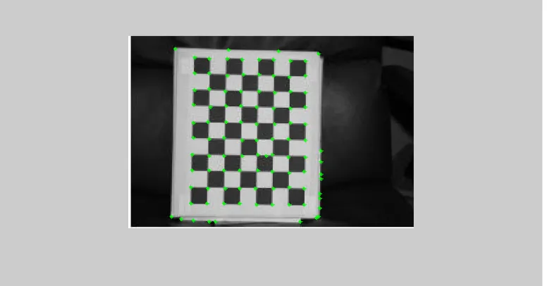
Harris corner detector algorithm is evaluated on the testing images collected from [2].

The values used to detect corners are k=0.04, size of the smoothing window = 3,  =1,

threshold = 6.2411e+009.

Local maximum cornerness values are collected and are sorted. Based on the number of

corners the threshold value is assumed. In this case 2000 corners are detected. Hence

from the list of all corner values the higher 2000 values are considered as corners and

14

Figure 3. Corner detection using harris corner detector

For a checkered board image the number of corners detected is 100.

15 2.4 Conclusions

Harris corner detector is widely used to detect corners over other corner detectors due to its

invariance properties. However, it is sensitive to noise as it depends on gradient information.

From the above two images we can observe that all the corners are detected in checkered board

image but where as in the other image few outliers are detected as corners. If the threshold and

the value of k is improved then the outliers in the corners can be decreased. Sensitivity to the

noise can be reduced by using a larger window, but this will further increase the computational

16

Chapter 3 2D and 3D Vision Formation

3.1 Simple camera system-pinhole model

A camera model is a mathematical formulation which approximates the behavior of a CCD

camera by using a set of mathematical equations. It is a projective mapping from a 3D projective

space 3

to a 2D projective space 2

. In order to understand how points in the real world are

related mathematically [4] to points on the imaging screen two coordinate systems are of

particular interest.

 The world coordinate system denoted by Wwhich is independent of camera parameters

(WCS).

 The camera coordinate system denoted by C(CCS).

Assume a point P_W with coordinates





the coordinates





related by

17

Figure 5. Simple pinhole camera model [4]

In the above figure, the point C_{is called the} central or focal point, along with the axes X_C,Y_C

and ZCdetermine the coordinate system of the camera. The image plane is parallel to plane

,

C C

X Y and located at a distance f from the optical center, and the z-axis of CCS coincides with

the optical axis. The distance between the image plane and the focal point is known as the focal

length.

The measurements obtained from the images are in pixel values expressed in natural numbers.

The projection of the point C on the plane  in the direction of z_camdefines the principal point

of the local coordinates





single pixel.

The projection of point PCon the image plane  is an image point Pim.

18 P_𝐶 = 𝑋_𝐶 𝑌_𝐶 𝑍_𝐶

P_𝑖𝑚 = 𝑥_𝑖𝑚 𝑦_𝑖𝑚 𝑧_𝑖𝑚

According to similar triangles, these coordinates are related as

C C

im im

C C

X Y

x f y f

Z Z

 

0 0 0

0 0 0

1 0 0 1 0

1

C im

C C im

C

X

x f

Y

Z y f

Z

 

   _{  }

  _{   }

   _{  }

   _{  }

   

 

Since the coordinate Z_C is usually unknown we can replace Z_Cby arbitrary positive scalar.

The above equation constitutes the pinhole camera model.

The pinhole camera model can be defined by two set of parameters:

 External camera parameters

 Internal camera parameters

3.1.1 External parameters

The mathematical relation between the chosen reference coordinate system and the camera

coordinate system can be expressed in terms of External Parameters. With respect to the world

reference system and the position of the image plane the camera coordinate system can be

located.

If we have more than one camera, without loss of generality we can consider the camera one

coordinate system to be the reference system. The relative pose and location between cameras

19

Transformation from the camera coordinate system to the external world coordinate system can

be attained by a translation Tand a rotationR. By multiplying the rotation matrix with the axes

of the reference coordinate system a new coordinate system is formed. The rotation matrix is an

orthogonal matrix. For a given point P_W , its coordinates in the camera coordinate system relative

to the world coordinate system is given by





P_C  R T P_W

The matrices R and T can be specified as

1 11 12 13

2 21 22 23

3 31 32 33

r r r r

R r r r r

r r r r

        _{  } _         and x y z T T T T           

11 12 13

21 22 23

31 32 33

1 0 0 0 1 1

C x W

C y W

C z W

X r r r T X

Y r r r T Y

Z r r r T Z

              _                      (2)

Hence, the external parameters of the camera are all geometric necessary parameters which

describe the transformation from the camera coordinate system to the world coordinate system.

3.1.2 Rotation matrix

The rotation matrix represents the orientation of an object or a frame with respect to the

reference frame. A rotation matrix has nine elements but all elements are not independent. There

are six constraints on the nine elements. Hence the degree of freedom is 3. There are different

sets of parameters that can be used to representing a rotation.

They are

20

3.1.3 Rotation matrix representation using Euler angles

Leonhard Euler (1707-1783) reasoned that the rotation from one frame to another can be

visualized as a sequence of three simple rotations about base vectors.

Each rotation is through an angle (Euler angle) about a specified axis. Let us consider the

rotating coordinate axes from X to _W X by means of three Euler angles. The first rotation is _C

about zaxis and rotated through an angle of _z. The rotation matrix about z axis is represented

as

cos( ) sin( ) 0 ( ) sin( ) cos( ) 0

0 0 1

z z

z z z z

R

 

  

 

 

 _{ }

 

 

The resulting frame is

1

C W

X R_z(_z)X

The second rotation is about yaxis through an angle _y. The rotation matrix is represented as

cos( ) 0 sin( )

( ) 0 1 0

sin( ) 0 cos( )

y y

y y

y y

R

 



 

  

 

  

 

 

The resulting frame is X_C2 R_y(_y)X1_CR_y(_y)R_z(_z)X_W

21

1 0 0

( ) 0 cos( ) sin( ) 0 sin( ) cos( )

x x x x

x x

R   

             

The resulting frame is X_C3 R_x(_x)X_C2 R_x(_x)R_y(_y)R_z(_z)X_W

Hence the final frame is X_C Rx(x)Ry(y)Rz(z)X_W

3.1.4 Intrinsic parameters

The mapping [4] from the image coordinates to the pixel coordinates is described. The pixel and

image coordinates are related by

0 P

1 0 0 1

p x x im

p y y im C

x s s o x

y s o y K

f           _   _                   (3) where, 0

0 0 1

x x

y y

s s o

K s o

           

is the internal calibration matrix. These are called internal parameters because they are fixed and

independent of placement and orientation of camera.









s_: skew of the pixel, often considered to be zero.

The projective Transformation of the pinhole camera is

22

Pp K R T[ ]PW

Kis the internal calibration matrix. The matrix





Kdefines the intrinsic parameters of the pin-hole camera, that is, the distance of the camera

plane to the centre of the camera coordinate system, as well as placement of the central point o

and the physical dimensions of the pixels on the camera plane. The external parameter matrix of

the pin-hole camera relates the camera and the external „world‟ coordinate systems. The three

equations above can be joined together as follows:

1

2

3 0

0

1 0 0 1

1

W

p x x x

W

p y y y

W z

X

x fs o r T

Y

y fs o r T

Z r T         _{  }   _   _{  }      _{  }      _{  }         1 2 3 0 0

1 0 0 1

1

W

p x x x

W

p y y y

W z

X

x o r T

Y

y o r T

23

Chapter 4 Feature Matching

The feature point matching problem consists in finding pairs, among many candidate feature

points, that correspond to the same scene element. The features [33] from both the reference

image and the sensed image are detected. These features can be matched based on their image

intensity values in their close neighborhoods.

For both the reference and sensed images Im and ₁ Im the correlation is calculated based on the ₂

window size. All corners within certain disparity limit are compared over two images. The

strength of a match is obtained by cross correlation of the image intensity over two pixel patches

on each feature.

The most common matching measures for intensity signals are

 Sum of Absolute differences









1 2

W , ,

SAD i i i i

D 



 Sum of squared differences





1 2

W ( , ) ( , )

SSD i i i i

D 



 Normalized sum of squared distances













i i i i

SSD N

i i i i

I x y I x x y y

D

I x y I x x y y

24

Feature matching is an important step for automated detection and tracking. In this thesis, an

25

Chapter 5 Stereo Vision

In order to infer the information regarding the depth, at least two cameras are required which are

located at distinct points monitoring the same scene. If only one camera is monitoring, without

the knowledge of geometry of the scene one cannot recover the depth information.

5.1 Epipolar geometry

The epipolar geometry [4] is the intrinsic projective geometry between two views. It is

independent of the scene structure, and only depends on the camera internal parameters and

relative pose.

The fundamental matrix F encapsulates this intrinsic geometry. It is a 3 3 matrix of rank 2. If

a point in 3D space P_W is imaged as 1

Pim in the first view, and

2

Pim in the second, then the image

points satisfy the relation

1 2

P_imFP_im 0

26

The above figure has two pin-hole cameras, each composed of the projective plane i (where

subscript iis changed to l for the left and to rfor the right camera respectively) with the

respective projective centre pointO_i. The line passing through the point O_iand perpendicular to

the plane _i intersects this plane at a point called the principal point. The distance from this

point to the centre point O_iis called the focal length f . The line O O_{l r}connecting the centers‟ O_l

and Or is called the base line. Points of its crossing with the image planes i determine the

epipolar points. If the line O O_{l r}does not cross the image planes_i , the corresponding epipolar

points lie in infinity.

A plane formed by a given 3D point PW and the projective centers Oland Or is called the

epipolar plane _e . The intersection of image plane with the epipolar plane is called epipolar

line.

For a 3D point P_W, the corresponding image point in left camera isP_iml The camera centre O_land

left image pointPiml form a ray P l l im

O . It can be seen that the point Piml is an image of the point

P_W but also of all the other points on the rayOlPiml . This means that the point PW can lie

anywhere on this ray, with same image point. Hence to find the exact space position of point P_W

itis not possible having one image.

To estimate space position we need a second image point, viewed from another position. This is,

for example, an image pointPimr on the plane r The point P r

imand the second central point Or

determine the second ray OrPimr . This ray is fixed at Or and simultaneously it can slide through

the ray Pl l im

O , to find the space point P_W . Moreover, the crossing point of each ray Pl l im

27

Pr

r im

O with their respective image planes _l or _r lies on the epipolar lines. Similarly,

projections of these rays on the opposite image planes compose epipolar lines as well.

Projection of every point P_Wlies in the image plane and on the corresponding epipolar line.

With each of the cameras of the stereo system we attach a separate coordinate system with its

centre coinciding with the central point of the camera. The zaxis of such a coordinate system is

collinear with the optical axis of the camera. In both coordinate systems the vectors

Piml ximl yiml ziml 

 

   and Pimr ximr yimr zimr 

 

   represent the same 3D point PW. On the other hand,

on the respective image planes, the vectors P_iml  x_iml y_iml z_iml _ and P_imr  x_imr y_imr z_imr _ represent

the projection of point P_W. Additionally we notice that z_iml  f_l andz_imr  f_r, where f_l and f_rare

the focal lengths of the left and right cameras, respectively.

Each camera is described by a set of extrinsic parameters. They define location of a camera

relative to the world or reference coordinate system. On the other hand, each camera has its own

local coordinate system, it is possible to change from one coordinate system to the other by a

translation T O_r O_land rotation determined by an orthogonal matrixR. Thus, for the two

vectors Piml and P r

im pointing at the same point PWfrom 3D space the following holds

Pimr R(Piml T) (4)

The epipolar _e plane in the coordinate system associated with the left camera is spanned by

the two vectors T andP_iml . Therefore, also the vector





28







where





0

P 0 P

0

l

z y im

l l l

im z x im im

l

y x im

T T x

T T T y A

T T z

          _  _{ }   _     

Substituting above eqns. in eq. (4) we get





P P 0

P P 0

r l im im r l im im R A E   _ 

where E AR (5)

The eq. (5) is termed as Epipolar constraint

E is called Essential Matrix. It has rank two because matrix A has rank two.

5.1.1 Essential matrix estimation

Essential Matrix can be estimated based on eq. (5). It has nine elements which are to be

estimated. As the formulas are based on homogenous coordinates any solution is determined up

to a scale factor hence, the number of elements to be estimated has reduced to eight. It needs

eight matched pair of points to estimate Essential Matrix. Hence, this algorithm is named as eight

point algorithm. If more matched pairs are available least square method is to be employed.

 







 



3 3

1 1

( , ) 0

T

r l

im im

i j

P i E i j P j

 





It can be re written as 9 1 0 i i i q E  



29

If more than eight exact point correspondences are available, Essential matrix is estimated using

Least squares method. The constraint on norm is also imposed.

2

min qE Constrained to E 1

   

 

2 T _{T T}

qE  qE qE E q q E

From qthe moment matrix G = q qT is created which is of size 9 9 . According to Lagrange

Multipliers optimization solution constitutes a minimal eigen value of positive define matrixG .

This can be achieved by Singular value decomposition SVD algorithm. The solution for E

corresponds to the last column vector of matrix V in [U S V] = svd(G ) which is the eigen vector

of least eigen value of matrix G .

Rotation matrix and Translation vector are to be estimated from the Essential Matrix.

Let

0 1 0 1 0 0 0 0 1

zp R             and

0 1 0 1 0 0 0 0 1

zn R      _{ }    

There exist two possible solutions for Rotation matrix and Translation vector related to a nonzero

Essential matrix.

Singular value decomposition of Eis U V T









T T T

zp zp

skew T R  UR U UR V









T T T

zn zn

30

Hence, from E we can recover the pose up to four solutions. We can eliminate three other

solutions by imposing the positive depth constraint. All the points should lay in front of the

31

Chapter 6 Calibration Methods

Camera calibration is an important step in computer vision problems. Camera calibration

involves in finding the parameters that affects the imaging process. They are



_

_

 Usually it is not at the centre of the image (width/2, height/2)







Algorithms for camera calibration discussed in the literature can be categorized into two types.

They are

1. Calibration with a rig

2. Self calibration method or Auto calibration method.

6.1 Calibration with a rig

In this case the camera parameters [18] are estimated using an object of known geometry. The

object is a calibration object. Calibration objects can be a checkered board pattern arranged at

right angles, etc., whose position is known with precision. This type of camera calibration is

accurate if the position of points in the world is known accurately. If the correspondence between

the 3D – 2D image points is known for at least five points the camera parameters can be

32

includes 3 for rotation and 3 for translation and 4 for internal parameters) at least five

non-coplanar points are essential. If more than five points are available the least squares method can

be employed. Each 3D-2D point correspondence gives two equations.

11 12 13

31 32 33

x y

x y

z z

x

x im x x

z

r r r T

z x o f

r r r T

  

  

  

21 22 23

31 32 33

x y z

x y z

y

y im y y

z

r r r T

z y o f

r r r T

  

  

  

If more point correspondences are available then the number of equations are more than the

number of unknowns which makes the system an over determined system. We can solve it using

least squares by minimizing the cost function in terms of observed image points and estimated

image points:



 







ˆ ˆ

i i i i

x x y y

i

mi

e n



6.2 Self calibration

In many practical situations one cannot have access to the camera and hence calibration using a

rig is not possible. The information that is available is only the images. Under these

circumstances, if one has partial knowledge on the scene or camera, estimation of camera

parameters is possible. One has to admit that imposing such information may lead to errors if the

assumptions are not satisfied. In many instances one can find planar surfaces, parallel lines and

right angles which provide constraints on internal camera calibration Matrix. Additionally, if

33

some instances where camera is available but, some of the parameters of the camera like focal

length (while zooming) can change which makes impossible to calibrate with a rig.

6.2.1 Uncalibrated epipolar geometry

In the previous section we were discussing on the epipolar geometry for calibrated views. Here

we will derive epipolar geometry for uncalibrated views [4]. Epipolar constraint for uncalibrated views can be derived by extending the concept of calibrated camera‟s epipolar constraint. The

triple product formed by three vectors P , P_{r l} and Tis zero or in other words the vectors are

coplanar. Epipolar constraint is

2 1

P_rEP_r 0

1 P_r KP_p

2 1 1

P_pKTEKP_p 0

We know that E ARfrom eq. (5)

1

T

FK ARK

2 1 P_pFP_p 0

where A is the skew symmetric matrix of Translation vector. Given eight non-coplanar

corresponding pairs in two images, Fundamental matrix can be estimated using eight point

Algorithm. Fundamental matrix encapsulates the information regarding relative pose and

34 6.2.2 Properties of fundamental matrix

 Matrix size is3 3 . Rank of the matrix is 2.

 Fundamental matrix transfers the image point in first view to a vectorl₂ FP1_p. The

vector l₂ is a line in the image plane formed by image points P_p2such that it satisfies

2 2Pp 0

l  . In the similar way, Fundamental matrix transfers the image point in second

view to a line l₁according toFP_p2. These lines are called as epipolar lines.

The first task is to compute camera matrices from fundamental matrix. Fis decomposed using

QR decomposition into an orthogonal and right triangular matrix.

LetF RS, RUdiag r s( , , ) EVT; T

SVZV .

0 1 0 0 1 0

1 0 0 1 0 0

0 0 1 0 0 0

E Z

 

   

   

_{ } _{ }

   

   

Singular value decomposition of RisRUdiag r s( , , ) EVT. As the rank of Fis 2. The smallest

eigen value has to be replaced by a value which is in between rand ssuch that the condition

number of matrix is as good as possible.

The projection matrices or camera matrices are





1 0

PM  I andPM₂[Udiag r s( , , ) EV U(0, 0, ) '] .

The camera parameters obtained by this method are not true parameters but are related to the true

35

There are different algorithms to estimate parameters of camera as explained above. If the access

to the camera is available calibration method using a rig is used as the problem of encountering

errors is less. If the camera is not available then self calibration methods can be employed. In this

report camera calibration using a rig is considered.

6.3 Camera calibration using nonlinear least squares

Problem formulation: Estimating camera‟s external and internal parameters given the position of

three points in reference coordinate system and their corresponding location in images.



 

 

 







1...

c c c c c c c c

x x y y x x y y

i n

e min z z z z z z z z

 _   





xis a vector of unknown parameters to be estimated by minimizing e

x = _ _x, _y,o o_x, _y, _az, _el_

Estimated image coordinates when observed from camera 1 is given by

1

1 1 1 1

11 12 13

1 1 1 1

31 32 33

x y z

ˆ

x y z

i x

x x x

z

r r r T

z o

r r r T

   

 

   (7)

1

1 1 1 1

21 22 23

1 1 1 1

31 32 33

x y z

ˆ

x y z

y i

y y y

z

r r r T

z o

r r r T

   

 

36

Estimated image coordinates when observed from camera 2 is given by

2

2 2 2 2

11 12 13

2 2 2 2

31 32 33

x y z

ˆ

x y z

i x

x x x

z

r r r T

z o

r r r T

   

 

   (9)

2

2 2 2 2

21 22 23

2 2 2 2

31 32 33

x y z

ˆ

x y z

y i

y y y

z

r r r T

z o

r r r T

   

 

   (10)

1 2

1 0 0 cos( ) cos( ) cos( ) sin( ) sin( )

0 1 0 sin( ) cos( ) 0

0 0 1 sin( ) cos( ) sin( ) sin( ) cos( )

el az el az el

az az

el az el az el

R R                      _{ } _  _        

1 1 1 11, 12, 13....

r r r are the elements of rotation matrix R₁. r r r₁₁2, ₁₂2, ₁₃2.... are the elements of rotation

matrix R₂. Rotation matrix has two degrees of freedom. World coordinate system is rotated

through an angle of _azabout zaxis and then rotated through an angle _elabout yaxis to form

the coordinate system for camera 2.

We wish to estimate the camera parameters in such a way that the projected 3D points are close

to the observed image coordinates. We employ Unconstrained Nonlinear optimization techniques

to estimate parameters. Levenberg Marquardt algorithm (LMA) provides solution to the problem

of minimizing a nonlinear function over a space of parameters of the function.

6.4 Experiment Results

Nonlinear least squares camera calibration algorithm is applied on the simulated data to evaluate

37

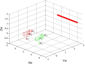
Simulation Setup: In this setup we have two pinhole cameras, looking at some feature points

whose location in world coordinates is known. First Camera pose w.r.t the world reference frame

is R1, T1 and the second camera pose w.r.t the world frame is R2, T2. Camera internal

parameters matrix is assumed to be same for both cameras K. By using projective geometry the

world points are projected to image plane located at z = 1. Here the optical axis is z-axis. Hence

the focal length f = 1.

We try to estimate cameras pose angles and camera internal parameters with the help of the

world coordinates of the feature points and their corresponding image coordinates. Internal

parameter matrix K =

50 0 250 0 50 250

0 0 1

 

 

 

 

 

Azimuth angle of camera 1 is –30degrees and for camera 2 is 30degrees and elevation angle for

camera 1 is 30degrees and for camera 2 is 30degrees.

Camera 1 is located at T1 =

0 0 0

         

.

Camera 2 is located at T2 =

2 0.7 0.3

 

 

 

 

 

Camera1 rotation angles are [azimuth1 elevation1] = _30 30 _

38

Feature points are projected to image plane according to perspective projection.

Figure 7. Simulation setup to estimate camera parameters

Figure 8. Camera 1 image coordinates

-1 0 1 2 0 1 2 3 -1 0 1 2 Yw 9 Y₂ X₂ 6 7 15 16 11 Z₂ 2 3 12 5 8 14 17 10 X W Y_W 1 4 13 Xw Z₁ Z_W X₁ Y₁ Zw camera 1 camera 2

39

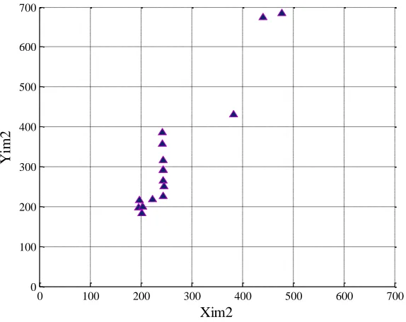
Figure 9. Camera 2 image coordinates

Measured coordinates are calculated using equations 7 through 10. Cost function is computed

using eq. (6). Cost function which is in terms of unknown camera internal and external

parameters is minimized to estimate the unknown values.

6.5 Conclusion

By using nonlinear least squares algorithm the camera internal and external parameters are

estimated. This algorithm gives good results when the location of feature points in 3D world

coordinates and their corresponding 2D coordinates are precise. If the location of the image

coordinates is not precise the estimated camera parameters are not true camera parameters. In

such case, nonlinear least squares give the local minimum value with certain residue. In the

above experiment we assume that the locations of ground truth points in 3D world coordinates

0 100 200 300 400 500 600 700 0

100 200 300 400 500 600 700

Xim2

40

and their corresponding 2D image locations are exact and hence the estimated camera parameters

41

Chapter 7 Object Tracking Model

The purpose of object tracking is to estimate the state of an object. An object dynamic model

describes [16] the trajectory of the object with respect to time. They assume that the motion of a

target can be described by a mathematical model known as state space models.

1 ( , )

( )

k k k k

k k k

x f x u w

z h x v

  

 

Here, xk, zk,ukare target state, observation and control input vectors in continuous time. f is

the state function model and h is the observation function that transforms the state space into the

observation space and w_kand v_kare the process and measurement noise respectively.

Target motions are categorized into maneuver and non-maneuver motions. In non-maneuver

motion a target moves in a straight line at constant velocity. All others fall into maneuver

category. In this project we assume that the target motion is constant over frames.

7.1 Nearly Constant velocity model

Let a point which is moving in the 3D world be described by its position and its velocity vectors.





x is a state vector where





space and





direction is considered zero. Target moves in xyplane. State space representation is

 

1

k k k

k k k

x Fx Gw

z h x v

  

42 2 2 2 0 0 2

1 0 0 0 0

0 0

0 1 0 0 0 0

0 0 1 0 0 0 0

2

0 0 0 1 0 0 _{0 0}

0 0 0 0 1

0 0

2 0 0 0 0 0 1

0 0 t t t t t F G t t _t t                                           

The above model is the nearly constant velocity model or “white acceleration model”.

Acceleration in xand ydirections is so small hence it is considered a nearly constant velocity

model.

7.2 Measurement model

The relation between the pixel coordinates and the 3D world coordinates is not linear. They are

related according to

11 12 13

31 32 33

21 22 23

31 32 33

x y

x y

z z

x y z

x y z

x x

z

x im x

y im y y

y

z

r r r T

f

r r r T

z x o

z y o r r r T

f

r r r T

                _{  }      _{  }    _{ }     _    (11)

The eq. (11) represents the measurement model equations. The Extended Kalman filter is similar

to a linearized Kalman filter, with the exception that the linearization is performed on the

estimated trajectory in the place of a previously estimated nominal trajectory. Extended Kalman

filter approximately linearizes the nonlinear function of the measurement locally according to

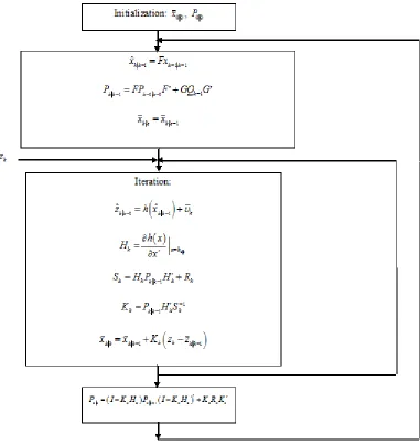
43 7.3 Iterative Extended Kalman filter estimation

In standard EKF xˆ_k xˆ_{k k1}is used in calculating the value of zˆ_{k k1}as ˆx_{k k}is not yet available. The

measurement prediction, up to the first order, is prone to errors in using this way. Other errors

may cause due to nonlinearity of the measurement model. The Iterated Klaman Filter method

uses Newton-Raphson algorithm to estimate ˆx_{k k}. The IEKF usually is better than EKF and the

level depends on the scenario that it is applied.

44

Figure 10. Algorithm for state estimation using Iterated Extended Kalman filter

7.4 Credibility of the filter

It is important [17] to evaluate the performance and characteristics of the algorithms used for

parameter, signal, and state estimation to serve a number of purposes, such as verification of its