Solving optimal control problems by PSO-SVM
Elham Salehpour∗
Department of Mathematics, Nowshahr branch, Islamic Azad university, Nowshahr, Iran. E-mail: [email protected]
Javad Vahidi
Iran University of Science and Technology, Information Technology Faculty, Tehran, Iran. E-mail: [email protected]
Hssan Hosseinzadeh Department of Mathematics,
University of Mazandaran, Babolsar, Iran. E-mail: [email protected]
Abstract The optimal control of problem is about finding a control law for a given system such that a certain optimality criterion is achieved. Methods of solving the optimal control problems are divided into direct methods and mediated methods (through other equations). In this paper, the PSO- SVM indirect method is used to solve a class of optimal control problems. In this paper, we try to determine the appropriate algorithm to improve our answers to problems.
Keywords. Particle Swarm Optimization, Support vector machines, Optimal control.
2010 Mathematics Subject Classification. 65L05, 34K06, 34K28.
1. Introduction
Theory of particle swarm optimization (PSO) has been growing rapidly. PSO has been used by many applications of several problems. The algorithm of PSO emulates from behavior of animals societies that don’t have any leader in their group or swarm, such as bird flocking and fish schooling. Typically, a flock of animals that has no leader finds food randomly by following one of the members of the group that has the closest position with a food source (potential solution). The flocks achieve their best condition simultaneously through communication among members who already have a better situation. Animal which has a better condition will inform it to its flock and the others will move simultaneously to that place. This would happen repeatedly until the best conditions or a food source discovered. The process of PSO algorithm in finding optimal values follows the work of this animal society. Particle swarm optimization consists of a swarm of particles, where particle represent a potential solution. Recently, there have been several modifications from original PSO.
Received: 13 January 2017 ; Accepted: 12 May 2018.
∗Corresponding author.
It was modified to accelerate the achieving of the best conditions. The development will provide new advantages and also the diversity of problems to be resolved. It is necessary to conduct studies on the development of PSO in order to recognize its development, advantages and disadvantages and the usefulness of this method to settle a problem. The theoretical tutorial of PSO is described in [1,2,3,4] testing the data is simpler, and has a simpler structure in comparison with other evolutionary computations.
Recently, Support Vector Machines (SVMs) were introduced by [14,19] for solving classification and nonlinear function estimation problems [6, 8, 9, 13]. Within this new approach the training problem is reformulated and represented in a way to obtain a (convex) quadratic programming (QP) problem. The solution to this QP problem is global and unique. In SVMs, it is possible to choose several types of kernel functions including linear, polynomial, RBFs, MLPs with one hidden layer and splines, as long as the Mercer condition is satisfied. Furthermore, bounds on the generalization error are available from statistical learning theory [7,17,18] which is expressed in terms of the VC (Vapnik- Chervonenkis) dimension. An upper bound on this VC dimension can be computed by solving another QP problem.
In this article, we mix SVM and PSO and with a new algorithm we study the problem of Narendra and Mukhopadhyay in 1997 which was solved by Suykens and his colleagues by LS-SVM [16]. Consider the following nonlinear system where x1,k andx2,k are the state variables anduk is the control variable:
x1,k+1= 0.1x1,k+ 2
u
k+x2,k 1+(uk+x2,k)2
x2,k+1= 0.1x2,k+uk
2 + u2k 1+x2
1,k+x
2 2,k
(1.1)
We are considering a new method in this paper to give a better answer. This paper is organized as follows:
In section 2, the N-stage optimal control problem is presented. In section 3, some works on support vector machines are reviewed. In section 4, PSO algorithm is studied.
In section 5, optimal control by support vector machines is studied.
In section 6, combining particle swarm algorithm with support vector machine is discussed.
In section 7, an example is presented.
2. The N-stage optimal control problem
In the N-stage optimal control problem is given one aims at solving the following problem is given [10]
min : ΨM(xi, ui) =τ(xM+1) +
M
X
i=1
f(xi, ui) (2.1)
s.t xi+1=ϕ(xi, ui), i= 1, . . . , M.
whereτ andf are positive definite functions. We will consider the quadratic cost
withP=PT >0,Y =YT >0.
The functionsτ, f andϕ are twice continuously differentiable. xi ∈ Rn denotes the state vector, ui ∈ R is the input of the system. This article is not limited to single-input systems.
In order to find the optimal control law, one constructs the Lagrangian
H(xi, ui, λi) = ΨM(xi, ui) + M
X
i=1
λTi [xi+1−ϕ(xi+ui)] (2.3)
where Lagrange multipliersλi∈Rn. The conditions for optimality are given [13]
∂HM
∂xM+1 = ∂f
∂xi +λi−1− ∂ϕ
∂xi T
λi = 0, i= 2, . . . M ∂HM
∂xM+1 = ∂r
∂xM+1 +λM = 0, ∂HM
∂ui =
∂f ∂ui −λ
T i
∂ϕ
∂ui = 0, i= 1, . . . M
∂HM
∂λi =xi+1−ϕ(xi, ui), i= 1, . . . M
(2.4)
For the case of a quadratic cost function subject to linear system dynamics with infinite time horizon, the optimal control law can be represented by full static state feedback control. However, in general, the optimal control law cannot be represented by state feedback as the optimal control law may also depend on the co-state. Never-theless, one is often interested in finding a suboptimal control strategy of this form. In the context of neural control [11,12,15].
ui=k(xi), (2.5) where k is a parametrized neural network architecture. In this paper, we will also consider a control law given in Eq.(2.5), to support vector machines. Because SVM methodology is not a parametric modeling approach, this is less straightforward in comparison with standard neural networks such as MLP’s and RBF’s.
3. The support vector machine
SVM algorithm was presented early in 1963 by Vladimir Vapnik. In 1995, he and his colleague extended the non-linear mode. SVM has very valuable properties which makes it suitable for pattern recognition.
SVM does not have local optimization problem in training. The category is built with maximum extension. The structure and topology are defined to optimize and the form of differential non-linear functions are calculated easily by using the concept of Hilbert spaces’ domestic multiplication. This is a supervised learning method used for classification and regression. This is a relatively new method. Compared to the older methods, the new method has been shown to have a good performance in recent years.
of dimensions. Large dimensions in a classification create a lot of parameters (when dimensions are increased, the covariance matrix becomes larger and more parameters must be calculated) that is difficult to estimate.
3.2. The users of SVM. The SVM algorithm is classified as the pattern recognition algorithm. SVM algorithm can be used wherever detecting patterns or categories of objects in specific classes is needed including risk analysis system, control plane with-out a pilot, track deviation plane, rwith-oute simulation, automatic guidance system for cars, quality in section systems, analysis of welding quality, quality forecast, quality analyzes computer, analysis of mill operations, chemical analysis of product design, analysis of maintenance, proposal, management and planning, chemical process, dy-namic control system, the design of artificial limbs, optimizing the time of organ transplantation, reducing hospital costs, improving the quality of hospitals, testing the emergency room, oil and gas exploration, automatic route control devices, robots, cranes, visual systems, voice recognition, concisely speech, classifieds sound, market analysis, consulting systems, calculating the cost of inventory, concise information and images, automatic information services, customer payment processing systems, truck brake detection systems, vehicle scheduling, routing systems, classifieds charts customer/market, drug recognition, signature verification, the loan risk estimation, spectral identification, investment appraise land so on [14,15,16].
3.3. Advantages and disadvantages.
1: Designing categories with maximum extension 2: Reaching the global optimal of cost function
3: Automatic determination structure and optimal topology of classifier 4: Modeling the non-linear differentiation function by using non-linear kernel
and concept of domestic multiplication in Hilbert spaces 5: Training is relatively simple
6: Unlike neural networks, it does not exist in local maximum 7: For high-dimensional data almost works good
8: Reconciliation between the complexity of product categories and the error is clearly controlled
9: Needs a good kernel function and select parameter C.
3.4. Support vector machine by linear classifier with linearly separable data:[14]. Suppose that we have the number of feature vectors or training patterns {x1, . . . , xM} and each of them is the m-dimensional feature vector and had labeled
yi, yi ∈ {−1,+1} . The purpose of solving optimization problem is in two classes. Suppose that we separate two classes with the differentiate functionf(X) and space
H with the following equation.
H:wx+b= 0
f(x) =wTx+b (3.1) If two examples of two classes with the names of (+1) and (−1) are expressed, these spaces can be considered as separate positive samples from negative samples.
So actually design is a hyper plane classification with border optimal which will be as follows:
min 1 2kwk
2
s.t yi(W Xi+b)≥1, i= 1,2, . . . M. (3.2) Clearly, we have:w= [w1, w2, . . . , wm]T and kwk2=wTwThe above problem can
be solved by quadratic programming (QP) optimization techniques. To solve it, this problem is written in the form of the following Lagrangian function and the Lagrange multipliers are obtained.
L(w, b, α) =1 2w
Tw− M
X
i=1
αi{yi(wTxi+b)−1}. (3.3)
The problem should be minimized in relation tob, w and αi variables should be maximized. We should solve this problem by eliminatingw,bvariables.
So the problem is a maximization problem. It will be based onαi. we solve this problem. To beL(w, b, α) the answer of the question, this answer must be true in KKT conditions and in the parts of the answer, L derive in relation to (α, b, w) is equal to. By equating the derivative to zero, we get the following equation:
L(w,b,α)
∂w = 0→w=
PM
i=1αiyixi,
L(w,b,α)
∂b = 0→w=
PM
i=1αiyi= 0.
(3.4)
By replacingwin the eq.(3.3), dual optimization issue will occur.
This formula of SVM is called difficult margin SVM. Because conducts classification completely and without any breach.
After solving the dual optimization issue, we reach to the Lagrangian coefficients. In fact, each of the coefficients αi is corresponding to one of the patterns xi that corresponds toαi >0 coefficients (positive) and are called support vectors sνi. [19]
The weight vector andbare obtained from the following relationship:
w=PMsv
i=1 αiyisvi,
bj=yj−P Msv
i=1 αiyisvisvj,
b= 1
Msv PMsv
j=1bj.
Distinction function will be classified by an input x pattern which is as follows:
f(X) =sign
Msv X
i=1
αiyiXsvi+b
!
. (3.5)
The linear classifier support vector machine with linearly in separable data (integral mode):
vector machine for the inseparable state. Now, we consider the case that we are still looking for a linear separating hyper plane with the difference that the separating hyper plane does not fully apply in inequality. To check this state, we define a new variable called Deficiency variableεi(slack variable) which represented the deviation from inequality (3.2). So the purpose of the algorithm is the maximum margin to define the payment of the cost appropriate to the deviation of inequality (3.2). It is clear that as long as the total amount of variables increases, the more error will occur which is far from optimal. The mathematical expression is in the form of the following:
min : Q(w, b, ε) = 1 2kwk
2+C
M
X
i=1 εpi,
s.t yi(wTxi+b)≥1−εi, εi≥0, i= 1, . . . , M, (3.6) whereε= (ε1, . . . , εM)T andcare margin parameters that determine the difference between the maximum margin and minimum error the classification.
To solve the equation, Lagrange multipliers are used
Q(w, b, ε, α, β) = kw2k2 +CPM
i=1εi−αi yi(wTxi+b)−1 +εi
−βiεi,
∂Q(w,b,ε,α,β)
∂w = 0, ∂Q(w,b,ε,α,β)
∂b = 0, ∂Q(w,b,ε,α,β)
∂ε = 0,
αi yi(wTxi+b)−1 +εi
, i= 1, . . . M,
βiεi= 0, i= 1, . . . M,
αi≥0, βi≥0, εi≥0, i= 1, . . . M. Respectively, we take partial derivatives in relation tow,b,ε.
w=PM
i=1αiyixi,
PM
i=1αiyi= 0,
αi+βi=C, i= 1, . . . , M. Replace and dual is written as follows:
max Q(α) = M
X
i=1 αi−
1 2 M X i=1 M X j=1
αiαjyiyjxTixj
s.t
M
X
i=1
This is the results that we mentioned below [20] 1: If αi= 0 thenεi = 0 in this casexi categorized.
2: If 0 < αi < C then yi(wTxi+b)−1 +εi = 0 and εi = 0 in this case
yi(wTx
i+b) = 1 and xi supportive vector. The support vectors with 0 <
αi< C is called a support vector boundless.
3: If αi = C then yi(wTxi+b)−1 +εi = 0 and εi = 0. So xi is a support vector. The support vectors withαi=C εi≥0,xi is classified and ifεi≥0, is a typed text or a website address or a translated document. It will not be classified.
4. Particle swarm optimization algorithm
Particle swarm optimization algorithm or PSO, also known as the swarm, is one of the most powerful and popular algorithms for optimization. This is mostly because the relatively high rate of convergence is used. These algorithms are a little old, but were successful in many application areas, older algorithms, such as genetic algorithms, surpass and were considered as the first choice.
PSO is one of the optimization methods inspired by nature which has been devel-oped for solving numerical optimization with very large search space without having to inform the gradient of the objective function. This was invented the first time in 1995 by two people named Kennedy and Eberhart. At the beginning, it was used to simulate the mass flight of birds. However, after the initial simple algorithm it was observed it was actually a type of optimization algorithm and for this reasons, it can also be used to solve other optimization problems.
The algorithm is inspired by the lives of a group of animals, including insects (such as ants, bees, etc.), birds and fish. To solve an optimization problem, a population of candidate solutions moves accidentally in the domain of problem using a simple formula, and explores it with aim of finding the global optimal answers. In PSO algorithm, each of these candidate answers is called a particle, and each particle flies with one of the birds in a flock as a corresponding answer. PSO algorithm is similar to genetic algorithms [1,3].
PSO algorithm is similar to genetic algorithm in the sense that a population of solutions is randomly generated by the algorithm and is looking for the answer by moving through the problem domain. However, unlike genetic algorithm, in the PSO algorithm a random velocity is assigned to each potential answer of optimization problem (in fact to each particle) in a way that in each repetition, each particle moves (or idiomatically flies) based on its velocity in the problem domain. Also, unlike genetic algorithm, in PSO algorithm, the best obtained answer for optimization problem must be stored by each of the particles (from the beginning of the program until the last repetition). Like genetic algorithm, PSO algorithm is also inherently suitable for solving the unconstrained maximization in continuous mode.
mathematical operators in order to adjust it to the minimum parameters required. In this method, minimum parameters are needed for adjustment. Furthermore, the executive function of algorithm will not be lost when the dimensions of research space are developed. PSO method is one of the new species of evolutionary methods whose application potential in optimization problems with continuous functions has been proved. In this way, move toward the optimal point, based on two data sets is done. One of the best-point of information obtained from each of the initial population [2,3].
An explanation on the PSO algorithm:
First, in the search space, a number of points are selected as the initial population. Points in different categories are based on Euclidean distance. For example i category includes three searching factors. The function value of each available factor in the search space is calculated and in each category, depending on the intended purpose, it is determined in which spot the value is minimized or maximized. Therefore, the best spot is identified for each category.
On the other hand, by accessing the previous information, each factor is able to locate the best spot that has been discovered so far. Thus, the optimal point information of each category and agent is specified. The first knowledge concerns the global optimal point in each group and the second knowledge concerns the local optimal point.
With this information, the motion vector is given to each factor. This method is not affected much by the size and nonlinear problem and has good results in static environments, noise and environments which are continuously changing. Simplicity of implementation, lack of commitment to the continuity of the objective function and the ability to adapt to a dynamic environment makes the algorithm useful in many different areas. Accordingly, it can be concluded that the targeted nature of the behavior of particles in PSO method is based on two principles [4].
These two principles are:
i . Individual knowledge: Each individual moves to the best of his knowledge to gain new knowledge.
ii . Social science: The person in terms of his relationship with the community uses the best information for continuing the movement.
In Article ii, Individual relationship with the community is important to the topology structure of the community, based on this, different topologies are defined for the society. This algorithm has advantages and disadvantages which are mentioned below [3,4].
Advantages algorithm include the following:
1: This algorithm is compared to other less regulated parameters optimized al-gorithms.
2: Implementation is easy and it has simple concepts. 3: It can be used effectively for various issues.
4: It is also used for discrete states and the continuum concepts.
6: The above algorithm optimization function application does not require any combination of information and only uses basic math operators.
7: It does not require heavy mathematical operations such as gradients. 8: It is a population-based approach.
9: The partnership uses particles.
According to mathematic law, in order to search for new solutions, the particle swarm optimization is valued randomly in search and movement space through D space. Assume that xi
k and ν i
k are respectively situation and particle speed of i in search space in k repetition then speed and situation of these particles will be updated in repetition (k+ 1) therefore, we will have following equations:
vT
i+1=w.vkT+c1.r1(pik−xik) +c2.r2.(pgk−xik),
xik+1=xik+vik+1.
wherer1 andr2 are the random number between 0 and 1 andc1 andc2are fixed, pi
k shows the best situation of i particle and p g
k relates to the best situation in the swap to k repetition.
One of the principle steps of particle swap optimization can be summarized as a pseudo code in algorithm 1.
Algorithm 1: Pseudo code of particle swarm optimization (PSO).
1: Objective function: f(x), x= (x1, x2, , xD);
2: Initialize particle position and velocity for each particle and set k= 1; 3: Initialize the particle’s best known position
to its initial position i.e. Pi k=X
i k; 4: do; 5: Update the best known position (Pi
k) of each particle and swarm’s best known position (Pkg);
6: Calculate particle velocity according to the velocity equation; 7: Update particle position according to the position equation;
8: While maximum iterations or minimum error criteria is not attained.
5. Optimal control by support vector machines Now, we are concerned with putting the training data{xi, yi}
p
i=1 in equation to
the state space and action space in Eq. (2.1), {xi, ui}Mi=1 . We state the following
N-stage optimal control problem:
min Ψ(xi, ui, w, ei) = ΨN(xi, ui) + 1 2w
Tw+1 2
M
X
i=1 e2i,
s.t xi+1=ϕ(xi, ui), i= 1, . . . , M, (5.1)
and the control law
where ΨM is defined in Eq. (2.1),w∈Rnf, f, g:
R→Rnf andn
f is the number of hidden units ofg. The actual control signal applied to bewTg(xi). In the linear control case hasg(xi) =xi withnf =n.
In the following, we will use RBF kernels. In the support vector method, applying the original Mercer’s condition is essential such that one does not have to construct g. Although the use of this kernel function will be proposed, it can assessgexplicitly, similar to the multilayer perceptron classifiers which is shown [9]. For the RBF case, Eq. (5.2) converts then
ui= nf X
r=1 wrexp
− 1
β2kxi−ark 2 2
+ei, (5.3)
wherear ∈Rn selection centers and β selection is constant. For example the set {ar}
nf
r=1 equal to {xi}Mi=1. In standard SVM theory for static function estimation
problemsβ can be selected so as to minimize an upper bound on the generalization error. These bounds are not applicable in the context of SVM control due to the fact that the input patterns to the activation function are not independent from each other. Henceβ should be chosen as hoc or could be taken as an additional unknown within the cost function.
In order to find the optimal control law we construct the Lagrangian
Ψ(xi, ui, w, ei, λi, γi) = ΨM(xi, ui) + 1 2w
Tw+
1 2
M
X
i=1 e2i +
M
X
i=1
λTi[ui−wTg(xi)−ei].
The conditions for optimality are
∂H
∂xi =
∂f
∂xi +λi−1−
∂ϕ ∂xi
T
λi−γi∂x∂
i[w
Tg(xi)] = 0, i= 2, . . . , M,
∂H
∂xM+1 = ∂r
∂xM+1+λM = 0,
∂H
∂ui =
∂f ∂ui−λ
T i
∂ϕ
∂ui +γi= 0, i= 1, . . . , M,
∂H
∂w =w−
PM
i=1γig(xi) = 0, ∂H
∂ei =αei−γi= 0, i= 1, . . . , M,
∂H
∂λi =xi+1−ϕ(xi, ui), i= 1, . . . , M,
∂H
∂γi =ui−w
Tg(xi)−e
i= 0, i= 1, . . . , M.
For RBF kernels
∂ ∂xi
[wTg(xi)] =−2X r
wrexp(− 1
β2kxi−ark 2 2)
xi−ar
The set of nonlinear
G1= (xi, xM+1, ui, w, ei, λi, γi) = 0, i= 1, , . . . , M. (5.5)
With givenx1and can numerically solve the unknown variables. In AppendixAa
formulation withoutei variables is given. In comparison with function estimation or classification problems, one looses the advantage of solving a quadratic program or a linear least squares problem. Nevertheless, one is still able to exploit some of the interesting SVM features.
As in SVM theory, Mercer’s condition can be replaced w = P
iγig(xi). in the equations.
For kernels satisfying Mercer’s condition
K(xi, xj) =g(xi)Tg(xj). (5.6)
For RBF kernels [5,7,17]
K(xi, xt) exp(−ϑkxi−xtk22), (5.7)
ν is a positive real constant
G2= (xi, xM+1, ui, λi, γi) = 0, i= 1, , . . . , M. (5.8)
By Mercer’s condition have [6]
∂f
∂xi+λi−1−(
∂ϕ ∂xi)
Tλ
i−γiPMt=1γt∂K∂x(xi,xt
i = 0, i= 2, . . . , M,
∂r
∂xM+1 +λM = 0,
∂f ∂ui −λ
T i
∂ϕ
∂ui +γi= 0, i= 1, . . . , M,
xi+1−ϕ(xi, ui) = 0, i= 1, . . . , M,
ui−P M
t=1αtK(xt, xi)−γαi = 0, i= 1, . . . , M.
(5.9)
For RBF kernels
∂K(xi, xt)
∂xi
=−2ϑ(xi−xt) exp(−ϑkxi−xt|22). (5.10)
The actual control signal applied to the plant becomes
ui= M
X
t=1
γtK(xt, xi), (5.11)
where{xt}Mt=1 and{γt}Mt=1 are obtained from solving the set of nonlinear Eq. (5.9)
and xi is the actual state vector at time i. The data {xt}Mt=1 are used as support
6. Combine PSO with SVM
According to the algorithm PSO, each particle has two elements: factors position and the objective function. In the proposed algorithm, the position of each particle is the starting point. We’re looking for an optimal position on the issue. To obtain value of objective function using the combination method of optimal control and support vector machine, the unknown factors and coefficients are calculated. Then by replac-ing it in the objective function, the costs are calculated. With the help of algorithm PSO, these steps are calculated for each particle, and finally the optimum starting point is achieved. As a result, the optimal starting point is placed in combination of SVM and optimal control, Finally, we obtain the optimal starting point. To solve the problem of optimal control using SVM, numerical methods using FMINCON function are used in MATLAB software.
Algorithm 2: Combine PSO with SVM.
1: Objective function: Optimal Control By LSSVM,x=x1, x2, . . . , xD;
2: Initialize particle position and velocity for each particle and setk= 1. 3: Initialize the particle’s best known position
to its initial position i.e. Pi k =Xki. 4: Do
5: Update the best known positionPki of each particle and swarm’s best known positionPkg.
6: Calculate particle velocity according to the velocity equation. 7: Update particle position according to the position equation.
8: While maximum iterations or minimum error criteria is not attained.
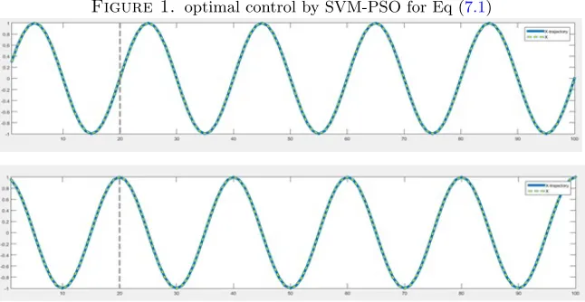
7. Simulation example Consider the following nonlinear system: [16]
x1,i+1= 0.1x1,i+ 2
u
i+x2,i 1+(ui+x2,i)2
,
x2,i+1= 0.1x2,i+ui
2 + u2i 1+x2
1,i+x22,i
. (7.1)
We consider a state vector tracking problem with
f(xi, ui) = (xi−xri) TP(x
i−xri) +u T i Y ui,
γ(xN+1) = (xN+1−xrN+1)
TP(x
N+1−xrN+1),
(7.2)
where xr
i is the reference trajectory. We aim at following these steps the first state variable and choose P = diag{1,0.001}, R = 1 for xr
i =
sin(220πk); cos(220πk)
with i = 1, . . . , N and N = 20. The given initial state is x1 = [0; 0]. As control
law is taken wTg([xi;xri]). In Figure 1, simulation results for method (5.9) show that Mercer’s conditions are useful. The set of nonlinear equations was solved using Matlab’s optimization toolbox (function leastsq) with unknownsxi, ui, λi, γ, β with
The unknowns were randomly initialized with zero mean and standard devia-tion 0.3. The plots show the simulation results for the closed-loop system ˆxi+1 = ϕxˆi,P
N
t=1αtK(xt,xˆi)
with RBF kernel. The controller is generalizing well with respect to other initial conditions where the origin (for which it has been trained) and time horizon forN = 20. The method (5.10) without the use of Mercer’s condition gave similar results by taking the centers{cr} equal to{xi}.
Figure 1. optimal control by SVM-PSO for Eq (7.1)
8. Conclusion
In this paper we introduced the use of combine support vector machines with particle swarm algorithm for solving optimal control problems. It is shown that this method is valuable in order to solve up timing problems of engineering design.
References
[1] B. Akay and D. Karaboga,Artificial bee colony algorithm for large-scale problems and engi-neering design optimization, Journal of Intelligent Manufacturing.,23(2012), 1001–1014. [2] J. S. Arora,Introduction to Optimum Design, McGraw-Hill, New York, 1989.
[3] A. Kaveh and S. Talatahari,Engineering optimization with hybrid particle swarm and ant colony optimization, Asian J. Civil Eng.(Build.Hous.),10(2009), 611–628.
[4] J. Kennedy and R. C. Eberhart,Particle swarm optimization, in: IEEE International Confer-ence on Neural Networks, Piscataway, NJ, Seoul, Korea, IV, 1995, 1942–1948.
[5] B. Scholkopf, K. K. Sung, C. Burges, F. Girosi, P. Niyogi, T. Poggio, and V. Vapnik, Compar-ing support vector machines with Gaussian kernels to radial basis function classifiers, IEEE Transactions on Signal Processing.,45(11) (1997), 2758–2765.
[6] B. Scholkopf, C. J. C. Burges, and A. J. Smola, Advances in kernel methods Support vector learning, Cambridge, MA: MIT Press, 1999.
[8] A. Smola, B. Scholkopf, and K. R. Muller,The connection between regularization operators and support vector kernels, Neural Networks.,11(4) (1998), 637–649.
[9] J. A. K. Suykens and J. Vandewalle,Training multilayer perceptron classifiers based on a mod-ified support vector method, IEEE Transactions on Neural Networks,10(4) (1999), 907–911. [10] J. A. K. Suykens and J. Vandewalle,Least squares support vector machine classifiers, Neural
Processing Letters., 9(3) (1999), 293-300.
[11] J. A. K. Suykens, B. De Moor, and J. Vandewalle,Static and dynamic stabilizing neural con-trollers, applicable to transition between equilibrium points. Neural Networks, 7(5), (1994). 819–831.
[12] J. A. K. Suykens, B. De Moor, and J. Vandewalle,NLq theory: a neural control framework with global asymptotic stability criteria, Neural Networks,10(4) (1997), 615–637.
[13] J. A. K. Suykens, L. Lukas, and J. Vandewalle,Sparse approximation using least squares support vector machines, IEEE International Symposium on Circuits and Systems ISCAS 2000, Geneva, Switzerland, 2000, 28–31.
[14] J. A. K. Suykens, L. Lukas, and J. Vandewalle,Sparse Least Squares Support Vector Machine Classifiers, 8th European Symposium on Artificial Neural Networks ESANN 2000, Bruges Bel-gium, 2000, 37–42.
[15] J. A. K. Suykens, J. Vandewalle, and B. De Moor,Artificial neural networks for modelling and control of non-linear systems, Boston: Kluwer Academic, 1996.
[16] J. A. K. Suykens, J. Vandewalle, and B. De Moor,Optimal control by least squares support vector machines, Neural Networks,14(1) (2001), 23–35.
[17] V. Vapnik,The nature of statistical learning theory, New York: Springer., 2000. [18] V. Vapnik,Statistical learning theory, New York: Wiley, 1998.
[19] V. Vapnik,The support vector method of function estimation, In J. A. K. Suykens and J. Van-dewalle, Nonlinear modeling: advanced blackbox techniques. Boston: Kluwer Academic, 1998, 55-85.