https://doi.org/10.5194/gmd-12-4261-2019 © Author(s) 2019. This work is distributed under the Creative Commons Attribution 4.0 License.
Fast domain-aware neural network emulation of a planetary
boundary layer parameterization in a numerical
weather forecast model
Jiali Wang1, Prasanna Balaprakash2, and Rao Kotamarthi1
1Environmental Science Division, Argonne National Laboratory, 9700 South Cass Avenue,Lemont, IL 60439, USA 2Mathematics and Computer Science Division, Argonne National Laboratory, 9700 South Cass Avenue,
Lemont, IL 60439, USA
Correspondence:Rao Kotamarthi ([email protected]) Received: 27 March 2019 – Discussion started: 29 April 2019
Revised: 10 August 2019 – Accepted: 1 September 2019 – Published: 10 October 2019
Abstract. Parameterizations for physical processes in weather and climate models are computationally expensive. We use model output from the Weather Research Forecast (WRF) climate model to train deep neural networks (DNNs) and evaluate whether trained DNNs can provide an accurate alternative to the physics-based parameterizations. Specifi-cally, we develop an emulator using DNNs for a planetary boundary layer (PBL) parameterization in the WRF model. PBL parameterizations are used in atmospheric models to represent the diurnal variation in the formation and collapse of the atmospheric boundary layer – the lowest part of the atmosphere. The dynamics and turbulence, as well as veloc-ity, temperature, and humidity profiles within the boundary layer are all critical for determining many of the physical pro-cesses in the atmosphere. PBL parameterizations are used to represent these processes that are usually unresolved in a typ-ical climate model that operates at horizontal spatial scales in the tens of kilometers. We demonstrate that a domain-aware DNN, which takes account of underlying domain structure (e.g., nonlocal mixing), can successfully simulate the verti-cal profiles within the boundary layer of velocities, temper-ature, and water vapor over the entire diurnal cycle. Results also show that a single trained DNN from one location can produce predictions of wind speed, temperature, and water vapor profiles over nearby locations with similar terrain con-ditions with correlations higher than 0.9 when compared with the WRF simulations used as the training dataset.
1 Introduction
Model developers use approximations to represent the phys-ical processes involved in climate and weather that can-not be resolved at the spatial resolution of the model grids or in cases where the phenomena are not fully understood (Williams, 2005). These approximations are referred to as parameterizations (McFarlane, 2011). While these parame-terizations are designed to be computationally efficient, cal-culation of a model physics package still takes a good portion of the total computational time. For example, in the Com-munity Atmospheric Model (CAM) developed by the Na-tional Center for Atmospheric Research (NCAR), with a spa-tial resolution of approximately 300 km and 26 vertical lev-els, the physical parameterizations account for about 70 % of the total computational burden (Krasnopolsky and Fox-Rabinovitz, 2006). In the Weather Research Forecast (WRF) model, with spatial resolution of tens of kilometers, time spent by physics is approximately 40 % of the computational burden. The input and output overhead is around 20 % of the computational time at low node count (100s) and can in-crease significantly at higher node count as a percentage of the total wall-clock time.
2011) that can reduce the time spent in calculating the phys-ical processes will lead to much faster model simulations, enabling researchers to generate high spatial-resolution sim-ulations and a large number of ensemble members.
A neural network (NN) is composed of multiple layers of simple computational modules, where each module trans-forms its inputs to a nonlinear output. Given sufficient data, an appropriate NN can model the underlying nonlinear func-tional relationship between inputs and outputs with mini-mal human effort. During the past 2 decades, NN techniques have found a variety of applications in atmospheric science. For example, Collins and Tissot (2015) developed an artifi-cial NN by taking numerical weather prediction model (e.g., WRF) output as input to predict thunderstorm occurrence within a few hundreds of square kilometers about 12 h in ad-vance. Krasnopolsky et al. (2016) used NN techniques for filling the gaps in satellite measurements of ocean color data. Scher (2018) used deep learning to emulate the complete physics and dynamics of a simple general circulation model and indicated a potential capability of weather forecasts us-ing this NN-based emulator. NNs are particularly appealus-ing for emulations of model physics parameterizations in numer-ical weather and climate modeling, where the goal is to find a nonlinear functional relationship between inputs and out-puts (Cybenko, 1989; Hornik, 1991; Chen and Chen, 1995a, b; Attali and Pagès, 1997). NN techniques can be applied to weather and climate modeling in two ways. One approach involves developing new parameterizations by using NNs. For example, Chevallier et al. (1998, 2000) developed a new NN-based longwave radiation parameterization, NeuroFlux, which has been used operationally in the European Centre for Medium-Range Weather Forecasts four-dimensional varia-tional data assimilation system. NeuroFlux is found to be 8 times faster than the previous parameterization. Krasnopol-sky et al. (2013) developed a stochastic convection parame-terization based on learning from data simulated by a cloud-resolving model (CRM), initialized with and forced by the observed meteorological data. The NN convection parame-terization was tested in the NCAR Community Atmospheric Model (CAM) and produced reasonable and promising re-sults for the tropical Pacific region. Jiang et al. (2018) devel-oped a deep NN-based algorithm or parameterization to be used in the WRF model to provide flow-dependent typhoon-induced sea surface temperature cooling. Results based on four typhoon case studies showed that the algorithm reduced maximum wind intensity error by 60 %–70 % compared with using the WRF model. The other approach for applying NN to weather and climate modeling is to emulate existing pa-rameterizations in these models. For example, Krasnopolsky et al. (2005) developed an NN-based emulator for imitating an existing atmospheric longwave radiation parameterization for the NCAR CAM. They used output from the CAM simu-lations with the original parameterization for the NN train-ing. They found the NN-based emulator was 50–80 times
faster than the original parameterization and produced almost identical results.
We study NNs to emulate existing physical parameteri-zations in atmospheric models. Process emulators that can reproduce physics parameterization can ultimately lead to the development of a faster model emulator that can oper-ate at very high spatial resolution as compared with most current model emulators that have tended to focus on simpli-fied physics (Kheshgi et al., 1999). Specifically, this study in-volves the design and development of a domain-aware NN to emulate a planetary boundary layer (PBL) parameterization using 22-year-long output created by the WRF. To the best of our knowledge, we are among the first to apply deep neural networks (DNNs) to the WRF model to explore the emula-tion of physics parameterizaemula-tions. As far as we know from the literature available at the time of this writing, the only ap-plication of NNs for emulating the parameterizations in the WRF model is by Krasnopolsky et al. (2017). In their study, a three-layer NN was trained to reproduce the behavior of the Thompson microphysics (Thompson et al., 2008) scheme in the Weather Research and Forecasting (WRF) model using the Advanced Research WRF (ARW) core. While we fo-cus on learning the PBL parameterization and developing domain-aware NN for the emulation of PBL, the ultimate goal of our ongoing project is to build an NN-based algo-rithm to empirically understand the process in the numeri-cal weather/climate models that could be used to replace the physics parameterizations that were derived from observa-tional studies. This emulated model would be computation-ally efficient, making the generation of large-ensemble simu-lations feasible at very high spatial/temporal resolutions with limited computational resources. The key objective of this study is to answer the following questions specifically for PBL parameterization emulation: (1) What and how much data do we need to train the model? (2) What type of NN should we apply for the PBL parameterization studied here? (3) Is the NN emulator accurate compared with the original physical parameterization? This paper is organized as fol-lows. Section 2 describes the data and the neural network developed in this study. The efficacy of the neural network is investigated in Sect. 3. Discussion and summary follow in Sect. 4.
2 Data and method 2.1 Data
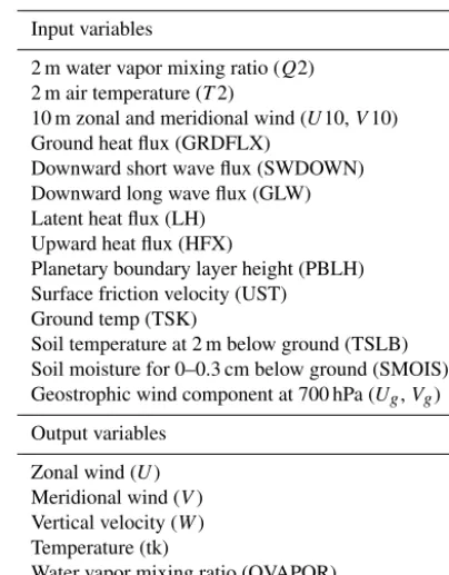
Table 1.Inputs and outputs for the DNNs developed in this study. The variable names from the WRF output are shown in the paren-theses.
Input variables
2 m water vapor mixing ratio (Q2) 2 m air temperature (T2)
10 m zonal and meridional wind (U10,V10) Ground heat flux (GRDFLX)
Downward short wave flux (SWDOWN) Downward long wave flux (GLW) Latent heat flux (LH)
Upward heat flux (HFX)
Planetary boundary layer height (PBLH) Surface friction velocity (UST)
Ground temp (TSK)
Soil temperature at 2 m below ground (TSLB) Soil moisture for 0–0.3 cm below ground (SMOIS) Geostrophic wind component at 700 hPa (Ug,Vg)
Output variables
Zonal wind (U) Meridional wind (V) Vertical velocity (W) Temperature (tk)
Water vapor mixing ratio (QVAPOR)
are 38 vertical layers, between the surface and approximately 16 km (100 hPa). The lowest 17 layers cover from the surface to about 2 km above the ground. The PBL parameterization we used for this WRF simulation is known as the Yonsei Uni-versity (YSU) scheme (Hong et al., 2006). The YSU scheme uses a nonlocal mixing scheme with an explicit treatment of entrainment at the top of the boundary layer and a first-order closure for the Reynolds-averaged turbulence equations of momentum of air within the PBL.
The goal of this study is to develop an NN-based emu-lator that can be used to replace the PBL parameterization in the WRF model. Thus, we expect the NN to receive a set of inputs that are equivalent to the inputs provided to the YSU scheme at each time step. Table 1 shows the ar-chitecture in terms of inputs and outputs used in our exper-iments. The inputs are near-surface characteristics including 2 m water vapor and air temperature, 10 m zonal and merid-ional wind, ground heat flux, incoming shortwave radiation, incoming longwave radiation, PBL height, sensible heat flux, latent heat flux, surface friction velocity, ground temperature, soil temperature at 2 m below the ground, soil moisture at 0– 0.3 cm below the ground, and a geostrophic wind component at 700 hPa. The outputs for the NN architecture are the ver-tical profiles of the following five model prognostic and di-agnostic fields: temperature, water vapor mixing ratio, zonal and meridional wind (including speed and direction), as well as vertical motions. In this study we develop an NN emula-tion of the PBL parameterizaemula-tion; hence we focus only on
predicting the profiles within the PBL, which is on average around 200 and 400 m during the night and afternoon of win-ter, respectively, and around 400 and 1300 m during the night and afternoon of summer, respectively, for the locations stud-ied here. The middle and upper troposphere (all layers above the PBL) are considered fully resolved by the dynamics sim-ulated by the model and hence are not parameterized. There-fore, we do not consider the levels above PBL height because (1) they carry no information about input/output functional dependence that affects the PBL and (2), if not removed, they introduce additional noise in the training. Specifically, we use the WRF output from the first 17 layers, which are within 1900 m.
2.2 Deep neural networks for PBL parameterization emulation
A class of machine learning approaches that is particularly suitable for the emulation of PBL parameterization is su-pervised learning. This approach models the relationship be-tween the outputs and independent input variables by using training data (xi,yi), forxi∈T⊂D, where T is a set of train-ing points, D is the full dataset, andxi andyi=f (xi)are inputs and their corresponding outputyi, respectively. The functionf that maps the inputs to the outputs is typically unknown and hard to derive analytically. The goal of the su-pervised learning approach is to find a surrogate functionh for f such that the difference between f (xi)andh(xi)is minimal for allxi∈T.
Many supervised learning algorithms exist in the machine learning literature. This study focuses on DNNs. DNNs are composed of an input layer, a series of hidden layers, and an output layer. The input layer receives the inputxi, which is connected to the hidden layers. Each hidden layer receives inputs from the previous hidden layer (except the first hidden layer that is connected to the input layer) and performs cer-tain nonlinear transformations through a system of weighted connections and a nonlinear activation function on the re-ceived input values. The last hidden layer is connected to the output layer from which the predicted values are obtained. The training data are given to the DNN through the input neural layer. The training procedure consists of modifying the weights of the connections in the network to minimize a user-defined objective function that measures the predic-tion error of the network. Each iterapredic-tion of the training proce-dure comprises two phases: forward pass and backward pass. In the forward pass, the training data are passed to the net-work and the prediction error is computed; in the backward pass, the gradients of the error function with respect to all the weights in the network is computed and used to update the weights in order to minimize the error. Once the entire dataset passes both forward and backward through the DNN (with many iterations), one epoch is completed.
K hidden layers, where the input of theith hidden layer is from the{i−1}th hidden layer and the output of theith hid-den layer is given as the input of the{i+1}th hidden layer. The sizes of the input and output neural layers are 16 (=
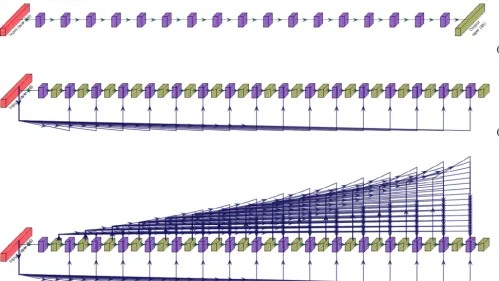
near-surface variables) and 85 (=17 vertical levels×5 out-put variables). See Fig. 1a for an illustration.
While the FFN is a typical way of applying NN for find-ing the nonlinear relationship between input and output, a key drawback is that it does not consider the underlying PBL structure, such as the connection between different vertical levels within the PBL. In fact, the FFN does not know which data (among the 85 variables) belong to which vertical level in a certain profile. This is not typically needed for NNs in general and in fact is usually avoided because, for classifi-cation and regression, one can find visual features regardless of their locations. For example, a picture can be classified as a certain object even if that object has never appeared in the given location in the training set. In our case, however, the location is fixed and the profiles over that location are distinguishable from the profiles over other locations if they are far from each other or have different terrain conditions. Consequently, it is desired to learn about vertical connection between multiple altitude levels within each particular PBL in the forecast. For example, the feature at a lower level of a profile plays a role in the feature at a higher level and can help refine the output at the higher level and accordingly the en-tire profile. This dependence may inform the NN and provide better accuracy and data efficiency. To that end, we develop two variants of DNNs for PBL emulation.
Hierarchically connected network with previous layer only connection (HPC). We assume that the outputs at each alti-tude level depend not only on the 16 near-surface variables but also on theadjacentaltitude level below it. To model this explicitly, we develop a DNN variant as follows: the input layer is connected to the first hidden layer followed by the output layer of size 5 (five variables at each layer: temper-ature, water vapor, zonal and meridional wind, and vertical motions) that corresponds to the first PBL. This output layer along with the input layer is connected to a second hidden layer, which is connected to the second output layer of size 5 that corresponds to the second PBL. Thus, the input to anith hidden layer comprises the input layer of the 16 near-surface variables and thei−1th output layer below it. See Figure 1b for an example.
Hierarchically connected network with all previous layers connected (HAC). We assume that the outputs at each PBL depend not only on the 16 near-surface variables but also on allaltitude levels below it. To model this explicitly, we mod-ify HPC DNN as follows: the input to an ith hidden layer comprises the input layer of the 16 near-surface variables and alloutput layers{1,2,},i−1}below it. See Fig. 1c for an ex-ample.
From the physical process perspective, HPC and HAC consider both local and nonlocal mixing processes within the PBL by taking into account not only the connection between
a given point and its adjacent point (local mixing) but also the connections from multiple altitude levels (e.g., surface and all the points that below the given points). Compared with solely local mixing processes, nonlocal mixing processes are shown to perform more accurately in simulating deeper mix-ing within an unstable PBL (Cohen et al., 2015). From the neural network perspective, the key advantage of HPC and HAC over FFN is effective back-propagation while training. In HPC and HAC, each hidden layer has an output layer; con-sequently, during the back-propagation, the gradients from each of the output layer can be used to update the weights of the hidden layer directly to minimize the error for PBL specific outputs.
2.3 Setup
For preprocessing, we applied StandardScaler (removes the mean and scales each variable to unit variance) and Min-MaxScaler (scales each variable between 0 and 1) transfor-mations before training, and we applied the inverse trans-formation after prediction so that the evaluation metrics are computed on the original scale.
We note that there is no default value forNunits in a dense hidden layer. We conducted an experimental study on FFN and found that settingN to 16 results in good predictions. Therefore, we used the same value ofN=16 in HPC and HAC.
For the implementation of DNN, we used Keras (ver-sion 2.0.8), a high-level neural network Python library that runs on top of the TensorFlow library (version 1.3.0). We used the scikit-learn library (version 0.19.0) for the prepro-cessing module. The experiments were run in a Python (Intel distribution, version 3.6.3) environment.
All three DNNs used the following setup for training: op-timizer: adam; learning rate=0.001; epochs=1000; batch size=64. Note that batch size defines the number of ran-domly sampled training points required before updating the model parameters, and the number of epoches defines the number of times that training will work through the entire training dataset. To avoid overfitting issues in DNNs, we use an early stopping criterion in which the training stops when the validation error does not reduce for 10 subsequent epochs.
The 22-year data from the WRF simulation was parti-tioned into three parts: a training set consisting of 20 years (1984–2003) of 3-hourly data to train the NN; a development set (also called validation set) consisting of 1 year (2004) of 3-hourly data used to tune the algorithm’s hyperparameters and to control overfitting (the situation where the trained net-work predicts well on the training data but not on the test data); and a test set consisting of 1 year of records (2005) for prediction and evaluations.
Figure 1.Three variants of DNN developed in this study. Red, yellow, and purple indicate the input layer (16 near-surface variables), output layers, and hidden layers, respectively.(a)Fully connected feed-forward neural network (FFN), which has only one output layer with 85 variables (five variables for each of the 17 WRF model vertical levels), and 17 hidden layers which only consider the near-surface variables as inputs.(b)Hierarchically connected network with previous layer only connection (HPC), which has 17 output layers (corresponding to the PBL levels) with each of them having five variables, and 17 hidden layers with each of them considering both near-surface variables and five output variables from previous output layer as inputs. (c) Hierarchically connected network with all previous layers connected (HAC); same as HPC, but each hidden layer also considers output variables fromallprevious output layers as inputs.
The DNN’s training and inference leveraged only a single GPU.
3 Results
In the following discussion we evaluate the efficacy of the three DNNs by comparing their prediction results with WRF model simulations. We refer to the results of WRF model simulations as observations because the DNN learns all the knowledge from the WRF model output, not from in situ measurements. We refer to the values from the DNN models as predictions. We initiate our DNN development at one grid cell from WRF output that is close to a site in the midwestern United States (Logan, Kansas; 38.8701◦N,100.9627◦W)
and another grid cell at a site in Alaska (Kenai Peninsula Borough; 60.7237◦N,150.4484◦W) to evaluate the robust-ness of the developed DNNs. We then apply our DNNs to an area with a size of∼1100 km×1100 km, centered at the Logan site to assess the spatial transferability of the DNNs. In other words, we train our DNNs using data from a sin-gle location and then apply the DNNs to multiple grid points
nearby. While the Alaska site has different vertical profiles, especially for wind directions, and lower PBL heights in both January and July (not illustrated), the conclusion in terms of the model performance is similar to the site over Logan, Kansas.
3.1 DNN performance in temperature and water vapor
Figure 2.Temperature and water vapor mixing ratio from the observation and three DNN predictions: FFN, HPC, and HAC in January and July of 2005 at 15:00 and 00:00 local time of Logan, Kansas. Theyaxis uses a log scale. The training data are from the 3-hourly output of WRF from 1984 to 2003. The lower and upper dashed lines show the lowest and highest (5th and 95th percentile) PBL heights at that particular time. For example, the lowest PBL height is about 19 m, while the highest PBL height is about 365 m at 00:00 in January.
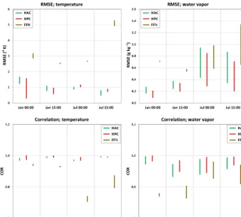
very low bias and high accuracy in the PBL; the FFN shows a relatively large discrepancy from the observation. Figure 3 shows the root-mean-square error (RMSE) and Pearson cor-relation coefficient (COR) between observation and three DNN predictions in the afternoon and midnight in January and July. The RMSE and COR consider not only the time se-ries of observation and prediction but also their vertical pro-files below the PBL heights for each particular time. Among the three DNNs, HPC and HAC always show better skill with smaller RMSEs and higher CORs than does FFN. The rea-son is that the FFN uses only the 16 near-surface variables as inputs; FFN uses all the 85 variables (17 layers×5 vari-ables/layer) as output without knowing the vertical connec-tions between each of the altitude levels. In contrast, HPC and HAC use both the near-surface variables and the five output variables of one previous vertical level (HPC) or all previous vertical levels (HAC) as inputs for predicting a cer-tain altitude level of each field. This architecture is helpful for reducing errors of each hidden layer during the backward propagation. It is also important because PBL parameteriza-tions are used to represent the vertical mixing of heat,
mois-ture, and momentum within the PBL, and this mixing can be across a larger scale than just the adjacent altitude levels. This process is usually unresolved in a typical climate and in weather models that operate at horizontal spatial scales in the tens of kilometers. We found in general that HAC and HPC perform similarly; the RMSE of temperature predicted by HAC is larger than that predicted by HPC during mid-night of winter when the PBL is shallow. In contrast, during the afternoon of summer when the PBL is deep, the RMSE of temperature predicted by HAC is smaller than that pre-dicted by HPC. This emphasizes the importance of consider-ing a multi-level vertical connection for deep PBL cases in the DNNs.
3.2 DNN performance in wind component
Figure 3.RMSE and correlations for time series of temperature and water vapor vertical profiles within the PBL predicted by the three DNNs compared with the observations. The vertical lines show the range of RMSEs and correlations when considering the lowest and highest PBL heights (shown by the dashed horizontal lines in Fig. 2).
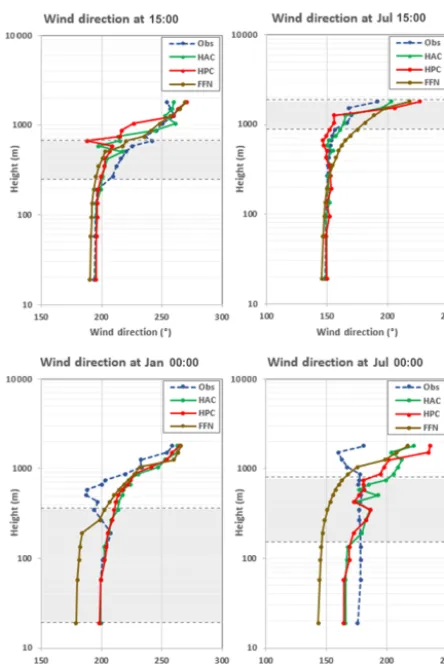
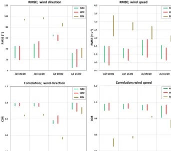
for days (e.g., summer) that have a higher PBL. The wind di-rection does not change much below the majority of the PBL, and it turns to westerly winds when going up and beyond the PBL. The DNN has difficulty predicting the profile above the PBL height, as is expected because these layers are consid-ered fully resolved by the dynamics simulated by the WRF model and hence not parameterized. Therefore, we do not consider DNN performance at the levels above PBL height. The wind speed increases with height in both January and July within the PBL. Above the PBL heights, the wind speed still increases in January but decreases in July. The reason is that in January the zonal wind, especially the westerly wind, is dominant in the atmosphere and the wind speed increases with height; in July, however, the zonal wind is relatively weak, and the meridional wind is dominant with southerly wind below∼2 km and northerly wind above 2 km. The de-crease in wind speed above the PBL is just about the transi-tion of wind directransi-tion from southerly to northerly wind. Fig-ure 5 shows the RMSEs and CORs between the observed and predicted wind component within the PBL. The wind compo-nent is fairly well predicted by the HAC and HPC networks with correlation above 0.8 for wind speed and 0.7 for wind direction except in July at midnight, which is near 0.5. Sim-ilar to the predictions for temperature and water vapor, the
FFN shows the poorest prediction accuracy with large RM-SEs and low CORs, especially for wind direction in July at midnight, the COR is below zero. For accurately predicting the wind direction, we found that using the geostrophic wind at 700 hPa as one of the inputs for the DNNs is important.
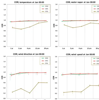
3.3 DNN dependence on length of training period
Figure 4.Same as Fig. 2 but for wind direction and wind speed.
and HPC also depend on the length of training data espe-cially when less than 6 years of training data is available, but even their worst prediction accuracy (using 1 year of training data) is still better than FFN using 20-year training data. The RMSEs of HPC and HAC predicted a temperature decrease from∼2.4 K using 1 year of training data to∼1.5 K using 20 years of training data. The CORs of FFN predicted a tem-perature increase from 0.73 using 1 year of training data to 0.92 using 20 years of training data. The CORs for HPC and HAC increase slightly with more training data, but overall they are above 0.85 using 1 year to 20 years of training data. Regarding the question about how much data one would need to train a DNN, for FFN, at least from this study, the performance is not stable until one has 12 or more years of training data, which is significantly better than having only 6 years or less of training data. For HAC and HPC, however, having 6 years of training data seems sufficient to show a sta-ble prediction. Increasing the amount of training data shows only a marginal improvement in predictive accuracy. In fact, in contrast to HAC and HPC, the performance of FFN has not reached a plateau even with the 20 years of training data. This suggests that with longer training sets the predicting skill of
FFN could be further improved even though it does not ex-plicitly consider the physical process within a PBL.
3.4 DNN performance for nearby locations
Figure 5.Same as Fig. 3 but for wind direction and wind speed.
in general, for temperature, water vapor, and wind speed, the domain-aware DNNs (HAC and HPC) still work fairly well for surrounding locations and even far locations with similar terrain height, except over the grid points where the terrain height is much higher than the Logan site, and the predic-tion skill gets worse with larger RMSEs. This suggests the DNNs developed based on the Logan site are not applicable for these locations. However, for wind direction, the predic-tion skill is good over the western part of the tested area, but it is not so good over the far eastern part of the area. One of the reasons is perhaps because the drivers of the wind direction over the western and the eastern part of the area are differ-ent (complex terrain versus large-scale system). Overall, the results indicate that, at least for this study, as long as the ter-rain conditions (slope, elevation, and orientation) are similar, the DNNs developed based on one single location can be ap-plied with similar prediction skill for locations that are as far as 520 km away (equal to more than 40 grid cells in the WRF output used in this study) to predict the variables assessed in this study. The results also suggest that when implementing the NN-based algorithm into the WRF model, if a number of grid cells are over a homogenous region, one may not need to train the NN over every grid cell. This will save a significant amount of computing resource because the training process takes up the majority of the computing resources (see below). While we show results predicted by HAC in January here, we
find a similar conclusion from HPC prediction and both HAC and HPC predictions in July, expect that the prediction skills are even better in July for the adjacent locations.
3.5 DNN training and prediction time
Figure 6.RMSEs for temperature, water vapor, and wind components at midnight in January using three DNNs. Leftyaxis is for RMSEs of HAC and HPC; rightyaxis is for RMSEs of FFN. The RMSEs are calculated along the time series below the PBL height for January midnight at local time. The lower and upper end of the dashed lines are RMSEs that consider the lowest and highest PBL heights as shown in Fig. 2.
Table 2.Training and prediction time (unit: seconds) for the three DNNs using a different number of years for training. The predicted period is for 1 year (2005).
DNN type Training data Training Number of Training time Prediction
(years) time epochs per epoch time
FNN 1 85.969 61 1.409 0.197
FNN 2 137.359 47 2.923 0.196
FNN 6 376.209 70 5.374 0.171
FNN 12 199.468 23 8.673 0.193
FNN 20 306.665 27 11.358 0.199
HPC 1 199.152 178 1.119 0.336
HPC 2 454.225 91 4.991 0.343
HPC 6 1233.908 133 9.278 0.317
HPC 12 1225.880 88 13.930 0.302
HPC 20 1181.716 68 17.378 0.331
HAC 1 131.104 95 1.380 0.366
HAC 2 468.884 85 5.516 0.411
HAC 6 870.753 80 10.884 0.406
HAC 12 737.921 47 15.700 0.420
Figure 7.Same as Fig. 6 but for Pearson correlations.
The prediction times of FNN, HPC, and HAC are within 0.5 s for 1-year data, making these models promising for PBL emulation deployment. The difference in the prediction time between models can be attributed to the number of pa-rameters in the DNNs: the larger the number of papa-rameters, the longer the prediction time. For example, the prediction times for FFN are below 0.2 s when using different numbers of years for training, while those for HAC are around 0.4 s. Despite the difference in the number of training years, the number of parameters for a given model is fixed. Therefore, once the model is trained, the DNN prediction time depends only on the model and the number of points in the test data (1 year in this study). Theoretically, for the given model and the test data, the prediction time should be constant even with different amounts of training dataset. However, we observed slight variations in the prediction times that range from 0.17 to 0.29 s for FNN, 0.30 to 0.34 s for HPC, and 0.36 to 0.42 s for HAC, which can be attributed to the system software.
4 Summary and discussion
This study developed DNNs for emulating the YSU PBL pa-rameterization that is used by the WRF model. Two of the DDNs take into account the domain-specific features (e.g., nonlocal mixing in terms of vertical dependence between multiple PBLs). The input and output data for the DNNs are taken from a set of 22-year-long WRF simulations. We devel-oped the DNNs based on a midwestern location in the United States. We found that the domain-aware DNNs (e.g., HPC and HAC) can reproduce the vertical profiles of wind, tem-perature, and water vapor mixing ratio with higher accuracy yet require fewer data than the traditional DNN (e.g., FFN), which does not consider the domain-specific features. The training process takes the majority of the computing time. Once trained, the model can quickly predict the variables with decent accuracy. This ability makes the deep neural net-work appealing for parameterization emulator.
Figure 8. (a)Terrain height (in meters) over the tested area;(b) nor-malized RMSEs in percent (relative to their corresponding obser-vations) of HAC-predicted temperature, water vapor mixing ratio, wind direction, and speed at midnight in January. The star shows where the DNNs are developed (Logan, Kansas).
correlations than does FFN. The wind profiles are more dif-ficult to predict than the profiles of temperature and water vapor. For FFN, the prediction accuracy increases with more training data; for HPC and HAC, the prediction skill stays similar when having 6 or more years of training data.
While we trained our DNNs over individual locations in this study using only one computing node (with multiple
pro-Figure 9.Person correlations between observed and HAC-predicted temperature, water mixing ratio, wind direction, and speed for mid-night in January in 2005.
cessors), there are 300 000 grid cells over our WRF model domain, which simulated the North American continent at a horizontal resolution of 12 km. To train a model for all the grid cells or all the homogenous regions over this large do-main, we will need to scale up the algorithm to hundreds if not thousands of computing nodes to accelerate the training time and the make the entire NN-based simulation faster than the original parameterization.
at a very high spatial resolution with a short computing time period so as to provide the means for generating large-ensemble model runs.
Code and data availability. The data used and the code developed in this study are available at https://github.com/pbalapra/dl-pbl (last access: 25 March 2019).
Author contributions. JW participated in the entire project by pro-viding domain expertise and analyzing the results from the DNNs. PB developed and conducted all the DNN experiments. RK pro-posed the idea of this project and provided high-level guidance and insight for the entire study.
Competing interests. The authors declare that they have no conflict of interest.
Acknowledgements. The WRF model output was developed through computational support by the Argonne National Laboratory Computing Resource Center and National Energy Research Scien-tific Computing Center.
Financial support. This research has been supported by the U.S. Department of Energy, Office of Science (grant no. DE-AC02-06CH11357).
Review statement. This paper was edited by Richard Neale and re-viewed by two anonymous referees.
References
Attali, J. G. and Pagès, G.: Approximations of functions by a mul-tilayer perception: A new approach, Neural Networks, 6, 1069– 1081, 1997.
Chen, T. and Chen, H.: Approximation capability to functions of several variables, nonlinear functionals and operators by radial basis function neural networks, Neural Networks, 6, 904–910, 1995a.
Chen, T. and Chen, H.: Universal approximation to nonlinear opera-tors by neural networks with arbitrary activation function and its application to dynamical systems, Neural Networks, 6, 911–917, 1995b.
Chevallier, F., Chéruy, F., Scott, N. A., and Chédin, A.: A neural net-work approach for a fast and accurate computation of longwave radiative budget, J. Appl. Meteorol., 37, 1385–1397, 1998. Chevallier, F., Morcrette, J.-J., Chéruy, F., and Scott, N. A.: Use of a
neural-network-based longwave radiative transfer scheme in the EMCWF atmospheric model, Q. J. Roy. Meteor. Soc., 126, 761– 776, 2000.
Collins, W. and Tissot, P.: An artificial neural network model to pre-dict thunderstorms within 400 km2South Texas domains, Mete-orol. Appl., 22, 650–665, 2015.
Cohen, A. E., Cavallo, S. M., Coniglio, M. C., and Brooks, H. E.: A review of planetary boundary layer parameterization schemes and their sensitivity in simulating a southeast U.S. cold season severe weather environment, Weather Forecast., 30, 591–612, 2015.
Cybenko, G.: Approximation by superposition of sigmoidal func-tions, Math. Control Signal., 2, 303–314, 1989.
Hong, S.-Y., Noh, S. Y., and Dudhia, J.: A new vertical diffu-sion package with an explicit treatment of entrainment processes, Mon. Weather Rev., 134, 2318–2341, 2006.
Hornik, K.: Approximation capabilities of multilayer feedforward network, Neural Networks, 4, 251–257, 1991.
Jiang, G.-Q., Xu, J., and Wei, J.: A deep learning algorithm of neural network for the parameterization of typhoon-ocean feedback in typhoon forecast models, Geophys. Res. Lett., 45, 3706–3716, 2018.
Kheshgi, H. S., Jain, A. K., Kotamarthi, V. R., and Wuebbles, D. J.: Future atmospheric methane concentrations in the context of the stabilization of greenhouse gas concentrations, J. Geophys. Res.-Atmos., 104, 19183–19190, 1999.
Krasnopolsky, V. M. and Fox-Rabinovitz, M. S.: Complex hybrid models combining deterministic and machine learning compo-nents for numerical climate modeling and weather prediction, Neural Networks, 19, 122–134, 2006.
Krasnopolsky, V. M., Fox-Rabinovitz, M. S., and Chalikov, D. V.: New approach to calculation of atmospheric model physics: Ac-curate and fast neural network emulation of long wave radiation in a climate model, Mon. Weather Rev., 133, 1370–1383, 2005. Krasnopolsky, V. M., Fox-Rabinovitz, M. S., and Belochitski,
A. A.: Using ensemble of neural networks to learn stochas-tic convection parameterizations for climate and numerical weather prediction models from data simulated by a cloud resolving model, Adv. Artif. Neural. Syst., 2013, 485913, https://doi.org/10.1155/2013/485913, 2013.
Krasnopolsky, V. M., Nadiga, S., Mehra, A., Bayler, E., and Behringer, D.: Neural networks technique for fill-ing gaps in satellite measurements: Application to ocean color observations, Comput. Intel. Neurosc., 2016, 6156513, https://doi.org/10.1155/2016/6156513, 2016.
Krasnopolsky, V. M., Middlecoff, J., Beck, J., Geresdi, I., and Toth, Z.: A neural network emulator for microphysics schemes, 97th AMS annual meeting, Seattle, WA, 24 January 2017.
Lee, L. A., Carslaw, K. S., Pringle, K. J., Mann, G. W., and Spracklen, D. V.: Emulation of a complex global aerosol model to quantify sensitivity to uncertain parameters, Atmos. Chem. Phys., 11, 12253–12273, https://doi.org/10.5194/acp-11-12253-2011, 2011.
Leeds, W. B., Wikle, C. K., Fiechter, J., Brown, J., and Milliff, R. F.: Modeling 3D spatio-temporal biogeochemical processes with a forest of 1D statistical emulators, Environmetrics, 24, 1–12, 2013.
Scher, S.: Toward data-driven weather and climate forecasting: Ap-proximating a simple general circulation model with deep learn-ing, Geophys. Res. Lett., 45, 12616–12622, 2018.
Thompson, G., Field, P. R., Rasmussen, R. M., and Hall, W. D.: Explicit forecasts of winter precipitation using an improved bulk microphysics scheme. Part II: Implementationof a new snow pa-rameterization, Mon. Weather Rev., 136, 5095–5115, 2008.
Wang, J. and Kotamarthi, V. R.: Downscaling with a nested regional climate model in near-surface fields over the contiguous United States, J. Geophys. Res.-Atmos., 119, 8778–8797, 2014. Williams, P. D.: Modelling climate change: the role of unresolved