in the population sciences published by the Max Planck Institute for Demographic Research Konrad-Zuse Str. 1, D-18057 Rostock · GERMANY www.demographic-research.org
DEMOGRAPHIC RESEARCH
VOLUME 22, ARTICLE 15, PAGES 383-472
PUBLISHED 16 MARCH 2010
http://www.demographic-research.org/Volumes/Vol22/15/ DOI: 10.4054/DemRes.2010.22.15
Research Article
Projection of populations by level of
educational attainment, age, and sex
for 120 countries for 2005-2050
Samir KC
Bilal Barakat
Anne Goujon
Vegard Skirbekk
Warren Sanderson
Wolfgang Lutz
© 2010 Samir KC et al.
This open-access work is published under the terms of the Creative Commons Attribution NonCommercial License 2.0 Germany, which permits use, reproduction & distribution in any medium for non-commercial purposes, provided the original author(s) and source are given credit.
1 Introduction 384
2 Approach 386
3 Existing projections 390
4 Methodology 392
4.1 Raw data and adjustments 392
4.2 Educational fertility differentials 392
4.3 Educational mortality differentials 398
4.4 Migration assumptions 400
4.5 Educational progression assumptions 401
4.6 Mean years of schooling 403
5 Scenarios 405
5.1 Demographic scenario 405
5.2 Education scenarios 406
5.2.1 Constant enrollment number (CEN) scenario 406
5.2.2 Constant enrollment ratio (CER) scenario 407
5.2.3 Global education trend (GET) scenario 407
5.2.4 The fast-track (FT) scenario 411
5.3 A note on educational policy discontinuities since 1990 412
6 Results and discussion 413
6.1 Sample output 413
6.2 Discussion 416
7 Future refinements 430
8 Conclusions and outlook 431
References 433
Appendix A 442
Appendix B 444
Projection of populations by level of educational attainment,
age, and sex for 120 countries for 2005-2050
Samir KC1
Bilal Barakat2
Anne Goujon3
Vegard Skirbekk4
Warren Sanderson5
Wolfgang Lutz6
Abstract
Using demographic multi-state, cohort-component methods, we produce projections for 120 countries (covering 93% of the world population in 2005) by five-year age groups, sex, and four levels of educational attainment for the years 2005-2050. Taking into account differentials in fertility and mortality by education level, we present the first systematic global educational attainment projections according to four widely differing education scenarios. The results show the possible range of future educational attainment trends around the world, thereby contributing to long-term economic and social planning at the national and international levels, and to the assessment of the feasibility of international education goals.
1 Corresponding Author: Dr. Samir KC, Research Scholar, World Population Program, International Institute
for Applied Systems Analysis (IIASA), Schlossplatz 1, A-2361 Laxenburg, Austria, tel.: +43-2236-807-424, fax: +43-2236-71313, e-mail: [email protected].
2 Dr. Bilal Barakat, Research Scholar, World Population Program, IIASA; and Research Scholar, Vienna
Institute of Demography of the Austrian Academy of Sciences; e-mail: [email protected]. 3 Dr. Anne Goujon, Research Scholar, World Population Program, IIASA; and Research Scholar, Vienna
Institute of Demography of the Austrian Academy of Sciences; e-mail: [email protected]. 4 Dr. Vegard Skirbekk, Leader, Age and Cohort Change Project, IIASA; e-mail: [email protected].
5 Prof. Dr. Warren Sanderson, Departments of Economics and History, Stony Brook University, New York,
USA; and Institute Scholar, World Population Program, IIASA; email: [email protected]. 6 Prof. Dr. Wolfgang Lutz, Leader, World Population Program, IIASA; Director, Vienna Institute of
Demography of the Austrian Academy of Sciences; Professor of Applied Statistics, Vienna University of Economics and Business; and Professorial Research Fellow, Oxford Institute of Ageing;
1. Introduction
This paper is part of an ambitious, multiphase project, the aims of which include the production of a new national level dataset on educational attainment by age and sex for as many countries in the world as possible over the period 1970-2000, the analysis of these new data, the preparation of projections of educational attainment by age and sex for those countries through 2050, and the assessment of the likely effects of future changes in educational structure. The project is a joint effort of the World Population Program at the International Institute for Applied Systems Analysis (IIASA) and the Vienna Institute of Demography (VID). Version 1.0 of both the educational attainment reconstructions and projections is now complete.7 In this paper, we describe the
methods used for projecting the educational attainment distributions for 120 countries for the years 2000-2050 using the methods of multi-state demographic modeling (see Appendix C).
Education-specific population projections are important, both because the information they produce is of intrinsic and practical interest, and because taking education into account improves the accuracy of the population projection itself. The latter is true because all three fundamental demographic components of fertility, mortality, and migration are strongly affected by education. In most societies, fertility levels vary significantly between women with different education levels (Jejeebhoy 1995; Bledsoe et al. 1999). Not just the number of children, but also the timing of births and marriage are strongly influenced by education levels. With regard to mortality, many factors contribute to a general pattern of higher life expectancy among the more educated (for instance, Kitagawa and Hauser 1973; Ahlburg, Kelley, and Mason 1996; Alachkar and Serow 1988; Preston and Taubman 1994; Doblhammer 1997; Lleras-Muney 2005), relating to healthy behavior (Kenkel 1991; Lantz et al. 1998), the gathering and appreciation of medical information (Niederdeppe 2008), better access to health care (Cleland and van Ginneken 1988), higher urbanization, etc. Finally, the highly educated are more likely to migrate and to move greater distances, and they are less likely to return to their country of origin.
As a result, population projections may lead to substantively different results in the presence of education variables than in their absence. Without education, they may also be less useful than they could be otherwise. Education is one of the keys to development. Interactions have been demonstrated with most development dimensions, including human rights, health, democracy, culture, economic growth, etc. (Sen 1999; Collier and Hoeffler 2000). Conversely, educational processes are affected by all of the above. Health affects absenteeism. The government’s respect for human rights influences access to schools for minorities; as one of the largest items of public
spending, education is tied closely to the economic development of the country. As such, education is both a means and an end to development.
Accordingly, an understanding of the educational level of the population is important when speculating about future development trajectories. Recently, we prepared a database for the population subdivided by age, sex, and education for the period 1970-2000 (Lutz et al. 2007). Using the UN’s age and sex distribution for the period, the proportions of each age and gender group who had attained different levels of education were reconstructed from data on education distributions compiled in and around 2000 (United Nations 2005). The dataset has been used by many researchers in different fields for analyzing effects of education on different variables. By applying their insights to the education profiles of future populations, it becomes possible to engage in informed speculation on the opportunities for development over the next four decades in various regions of the world.
Since the effects of educational attainment can also be expected to differ by age (e.g., one might expect that the education of 25-34-year-olds should be more important for economic growth than that of persons beyond retirement age) as well as by sex, having full age details for men and women can be considered a great asset for a comprehensive projection of future economic growth prospects. While some partial efforts at projecting levels of educational attainment have been developed at a more aggregated level, in the past, projections over several decades by age, sex, and level of education were not available for a large set of countries, including both industrialized and developing countries (but see the section on existing projections for a discussion of the closest alternative).
This projection exercise focuses strictly on levels of educational attainment, which are measures of the quantity and formal level of schooling obtained. Educational quality also has an important effect on human capital. Standard measures of skills acquired— such as the PISA (Programme for International Student Assessment), PIRLS (Progress in International Reading Literacy Study) school performance databases, or IALS (International Adult Literacy Survey) for adults—are based on actual testing of samples of the population, and show strong variations between countries that could explain other differentials associated with education. While such datasets based on the direct testing of skills are so far only available for a small number of (mostly OECD) countries, efforts are underway (e.g., by the UNESCO Institute of Statistics) to collect this type of information for a larger number of countries. In the future, we plan to incorporate educational quality and skills assessed on the basis of testing into our measures for countries where data are available, but this will be done in a later phase of the project.
Section 4, the main body of the paper, describes our method. It begins with a concise summary of the different steps involved, and then discusses at some length the key dimensions of the method: the raw data and adjustments to the data, the assumptions made about fertility, and mortality differentials and migration. In addition, Section 4 outlines our approaches to dealing with the age when progressing to higher attainment categories, describes the different demographic and educational scenarios, and discusses current limitations that may be overcome in future revisions. Section 5 gives a brief discussion of selected results, and Section 6 presents some sensitivity analyses. The concluding section provides a short outlook on the kinds of studies that may be possible with these projections.
2. Approach
In this section, we briefly describe the general approach taken in producing these new educational attainment projections. Starting from one empirical dataset for each country for the year 2000, distributions by level of education are projected along cohort lines.
The projections are based on the demographic method of multi-state population projection. This approach was developed at IIASA during the 1970s, and is now widely accepted by technical demographers. Our baseline year providing the empirical starting point is 2000, the same as in our reconstruction of the education distribution in the past. This allows us to connect the backward and forward projections in a gapless time series. We chose 2000 as the base year, since the data for 2005 were not available for a vast majority of countries.
The basic idea of projection is straightforward. Assuming that the educational attainment of a person remains invariant after a certain age, we can, for example, derive directly the proportion of women without any formal education aged 50-54 in 2005 from the proportion of women without any formal education aged 45-49 in 2000. Again assuming that this proportion is constant along cohort lines, the proportion of women without education aged 95-99 in 2050 for the same cohort can be derived directly. In a similar manner, the proportions for each educational category and each age group of men and women can simply be moved to the next older five-year age group as we progress forward in time in five-year steps.
approach is adjusted to correct for these effects. The size of birth cohorts is dependent on the levels of education of women of childbearing age, where a negative relationship is traditionally observed. In projecting these cohorts forward, differential survival rates are applied to the education groups. The differentials are based on a comprehensive literature review, as well on modeling exercises based on past data. The details of these adjustments are provided in later sections.
The above treats the different education groups essentially as separate sub-populations. In addition, at younger years transitions between the education categories may occur. These are described in detail in later sections. The analysis is simplified by the assumption that changes in educational attainment are uni-directional; i.e., that individuals can only move from the ‘no education’ status to primary, and on to secondary and possibly to tertiary; but can never revert to a lower status.
In reality, the likelihood of an individual making the transition from one educational attainment level to the next highest is strongly dependent on the education of the parents. This educational inheritance mechanism is not, however, modeled explicitly here. Instead, the assumptions regarding the transition rates and their future development are statistically derived from the aggregate behavior of education systems in the past. Since this expansion is partly the result of the inheritance mechanism—i.e., the fact that many parents aspire for their children to reach an education level at least as high as they themselves did—inheritance is implicitly reflected in the projection, even though it is not formally part of the model. Such an approach appears preferable at this time because data on the aggregate growth patterns of education systems, on which assumptions for the future can be based, are much more readily available than robust data on the micro-process of educational inheritance.
The starting point for the projection is data collected for each country (typically around the year 2000) which gives the total population by sex, five-year age groups, and four attainment categories based on the current International Standard Classification of Education (ISCED 1997). These categories are no education, primary, secondary, and tertiary (see Table 1).
Table 1: Education categories Category Definition
No education (E1) No formal education or less than one year primary
Primary (E2) Uncompleted primary, completed primary (ISCED 1), and uncompleted lower
secondary
Secondary (E3) Completed lower secondary (ISCED 2), uncompleted and completed higher
secondary (ISCED 3/4), and uncompleted tertiary education
When a single set of categories is applied to all countries, regardless of their state of educational development, it is inevitable that some compromises will have to be made. Surveys used exclusively in developing countries have historically provided little differentiation at higher education levels. Conversely, data collected in industrialized countries may not differentiate below completed primary level. For the present purposes, the entire spectrum, from no education to completed tertiary, needs to be covered. At the same time, a large number of detailed categories would be unwieldy, and would limit the number of countries for which data are available. Consequently, a relatively small number of categories is used to cover the entire spectrum. This means that the categories are relatively broad. Note, for instance, that ‘primary’ does not refer to completed primary, but to having more than one year of primary schooling. Likewise, for the purposes of this study, ‘secondary’ refers to lower secondary, not completed upper secondary. As a result, the ‘secondary’ category is quite broad, encompassing ISCED levels 2-4. The reason for not splitting off ISCED 4 is that the distinction between ISCED 3 and 4 is one of the least clear-cut, and also that ISCED 4 programs “are often not significantly more advanced than programmes at ISCED 3” (UNESCO Institute for Statistics 2009:258). As a result, attempting to distinguish between ISCED 3 and 4 would have undermined the straightforward hierarchical interpretation of our education categories.
Our procedure for each country can be summarized as follows:
• A baseline population distribution by five-year age group, sex, and level of educational attainment is derived for the year 2000.
• For each five-year time step, cohorts move to the next highest five-year age group.
• Mortality rates are applied, specific to each age, sex, and education group, and to each period.
• Age, and sex-specific educational transition rates are applied.
• Age, sex, and education-specific net migrants are added to or removed from the population.
• Fertility rates are applied, specific to each age, sex, and education group, and to each period, to determine the size of the new 0-5 age group.
The aim of the projection is to obtain a dataset with the population distributed by five-year age groups (starting at age 15 and ending with the age group 100+), by sex, and by four levels of educational attainment over a period of 50 years in five-year intervals, from 2000 (base year) to 2050.
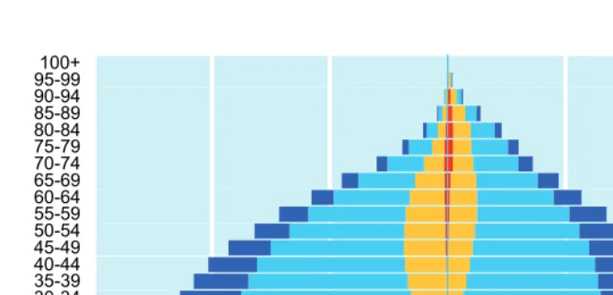
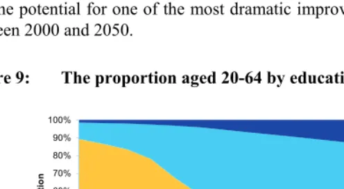
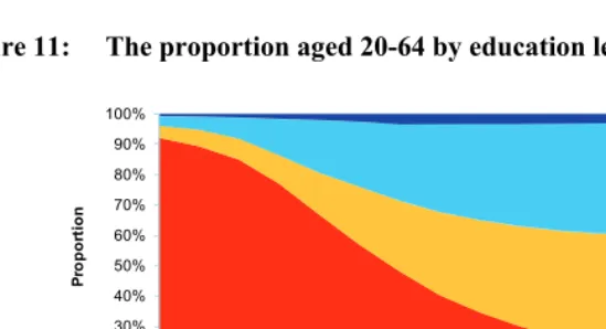
To illustrate the kind of information that this projection method generates for 120 countries in the world, Figure 1 gives an example in terms of age pyramids by level of education for South Africa. The first pyramid (Fig. 1a) shows the structure by age, sex, and level of education for the year 2000, which is the empirical baseline information used for the reconstruction. The second pyramid (Fig. 1b) gives the projected structure for the year 2050, resulting from our method.
Figure 1a: Structure by age, sex, and level of education for South Africa for the year 2000
3000 2000 1000 0 1000 2000 3000
15-19 20-24 25-29 30-34 35-39 40-44 45-49 50-54 55-59 60-64 65-69 70-74 75-79 80-84 85-89 90-94 95-99100+
Males Population in Thousands Females
Figure 1b: Projected structure for South Africa for the year 2050
3000 2000 1000 0 1000 2000 3000
15-19 20-24 25-29 30-34 35-39 40-44 45-49 50-54 55-59 60-64 65-69 70-74 75-79 80-84 85-89 90-94 95-99100+
Males Population in Thousands Females
No Education Primary Secondary Tertiary
3. Existing projections
improvements are rather small, as younger cohorts are almost as educated as older ones; whereas in other countries, like Spain, the scope for improvements is broader.
The multi-state approach, the base for the present projections, was developed at IIASA by Andrei Rogers (Rogers 1975), and was first applied in Mauritius by a group of IIASA researchers to human capital projections in a study of future development options, the so-called Population Development Environment (PDE) studies (Lutz 1994). It was then applied in Cape Verde (Wils 1996), the Yucatan Peninsula (Lutz, Prieto, and Sanderson 2000), Botswana (Sanderson, Hellmuth, and Strzepek 2001), Namibia (Sanderson et al. 2001), and Mozambique (Wils et al. 2001). Independently of those PDE studies, Yousif, Goujon, and Lutz (1996) used this methodology to project the population of six North African countries by age, sex, and education. Additional case studies include projections for India at the state level (Goujon and McNay 2003), for some countries in the Arab region (Goujon 2002), for China by urban and rural areas (Cao 2000), for Southeast Asia (Goujon and KC 2006), and for Egyptian governorates (Goujon et al. 2007). Several publications have aimed at evaluating this approach, such as Lutz, Goujon, and Doblhammer-Reiter (1999); and, more recently Lutz, Goujon, and Wils (2008). The method has been applied to produce the first global-level (for 13 world regions) projections by age, sex, and educational attainment to 2030 by Lutz and Goujon (2001).
By comparison, the current version of our projections focuses on education scenarios of a convergence to global trends (defined below), rather than on an extrapolation of country-specific trajectories. While less accurate with respect to individual countries in the short-term, this allows for greater coverage in the geographical and time dimensions, and permits us to draw broader conclusions about the global implications of changes in educational attainment. It may be argued that the EPDC approach is more suited to forecasting, while the present approach is more flexible with regard to engaging in ‘what if’ scenario reasoning regarding future global economic growth or health prospects.
4. Methodology
4.1 Raw data and adjustments
As a baseline for the projections, we need population distributions by age, sex, and level of educational attainment for all the countries included in the study. No single source of data provides this, so an integration of a diverse range of datasets was required. The baseline year 2000 was chosen partly because data for or around the year 2005 was not yet available for all countries at the time of data collection.
Various adjustments were necessary for creating the integrated year 2000 baseline dataset. These included adjustments for data from other years in the interval 1998-2002, the standardization of education categories, the mapping of data on 10-year age groups to our five-year age groups, the mapping of different aggregate ‘old age’ categories (such as 60+ versus 65+), and other minor corrections. Details of these adjustments, as well as the list of data sources, are documented in the report on the back-projection exercise (Lutz et al. 2007) and the validation exercises (Riosmena et al. 2008), with which the present projection shares the baseline dataset. Using this procedure, the starting populations by age, sex, and four levels of attainment for the year 2000 were obtained for 120 countries.
4.2 Educational fertility differentials
Office 1993; Smits, Ultee, and Lammers 2000; United Nations 1995). This relationship has been observed in countries at all stages of development, and from a wide range of cultural traditions. Several interrelated behavioral, economic, institutional, and social factors are likely to be at work. Education can affect preferences for fertility timing and outcomes, encourage female autonomy, increase contraceptive use, and raise the opportunity costs of childbearing (Goldin and Katz 2002; Jejeebhoy 1995; Skirbekk, Kohler, and Prskawetz 2004; Westoff and Ryder 1977).
The fertility impact of women’s schooling can be highly context-specific, varying by region of the world, level of development, and time (Jejeebhoy 1995). Women’s education may also be affected by cultural conditions, particularly by the position women occupy in a traditional kinship structure. Jejeebhoy further suggests that education affects fertility in a non-linear fashion, with some schooling leading to somewhat higher fertility, but additional schooling lowering it. Skirbekk (2008), however, tests this relationship based on 506 samples, and finds that schooling generally lowers fertility, even at the intermediary levels.
Jain (1981) and Gustavsson and Kalwij (2006) suggest that the labor market situation can explain the magnitude of the schooling-fertility relationship. Education is more negatively related to fertility the more opportunity costs increase with schooling, as is the case when employment and income correlates with educational levels. Moreover, a perceived negative relationship between children’s education and status and the number of children—i.e., the ‘quality versus quantity’ of offspring— could decrease fertility outcomes (Angrist, Lavy, and Schlosser 2006; Becker 1991). The very low fertility levels of highly educated women in countries characterized by below-replacement fertility is not likely to be intentional. Highly educated women have high— and, according to some evidence, higher—fertility ideals than others; it is realized fertility that is low (Noack and Lyngstad 2000; Symeonidou 2000; Testa and Grilli 2006; Van Peer 2002).
Demographic behavior in early adulthood has been characterized by a very typical sequence, in which the completion of education is followed first by entry into the labor market, and then by the birth of the first child (Marini 1984; Corijn 1996). Moreover, the global extension of education in recent decades has shifted the onset of this sequence to increasingly older ages. Consistent with this argument, Blossfeld and Huinink (1991) show that few women have children during their time in education.
to higher fertility among those with less schooling (Cleland 2001; Heer 1983). The less-educated are likely to be laggards in the fertility transition, and educational fertility differences may be indicative of a late fertility decline (Casterline 2001; Kravdal 2002).
The level of education is generally lower in developing countries, and increasing schooling from low levels rather than from medium levels can have stronger fertility-reducing implications (Cochrane 1979; United Nations 1995). Lower levels of education can be associated with less knowledge about reproduction and less access to contraception. Those with lower educational levels also tend to be less urbanized, are more likely to have traditional gender views, and are more prone to believe social status is increased by higher fertility (Birdsall and Griffin 1988; Cochrane 1979; Jejeebhoy 1995). Adherence to religious leaders and the belief that religious practice requires high fertility or prohibits contraceptive use have also been found to be more prevalent among the less-educated (Avong 2001; McQuillan 2004).
Education is likely to have a causal effect on both the timing and the outcome of fertility; however, its magnitude depends on the socioeconomic and cultural setting. Skirbekk (2008) finds that women’s fertility is, on average, significantly lower for the more educated—around 30% lower when the highest and the least educated groups are compared—and that this gap is even greater in poorer, high fertility contexts. The negative effect is stronger for Asia, Africa, Middle East, and Latin America than for Europe and North America. Relative fertility differentials by education persist for countries at the end of the fertility transition, albeit of somewhat smaller magnitude.
In explanations of the timing and level of fertility in developed countries, the role of education and human capital investments has often been emphasized. Despite the emphasis on the role of education in postponing and depressing fertility, only a few studies have identified the causal effects of the ‘age at school graduation’ on fertility patterns. Comparing individuals across educational attainment leads to selection problems, as individuals with more education also differ in terms of their preferences, abilities, labor market opportunities, and other factors relevant to the timing and outcome of fertility. Standard analyses of the relationship between education and fertility that compare individuals with different levels of educational attainment are therefore likely to be distorted, as many unobserved characteristics associated with higher graduation ages tend to be poorly measured or omitted. Analyses that overcome the above problem frequently rely on instrumental variable techniques, fixed-effect models, or ‘natural experiments’ (Rosenzweig and Wolpin 2000).
other factors on childbearing patterns. Often these studies rely on strong assumptions to identify any “causal influences” of education on fertility and human capital.
While the exact causal mechanism of the education-fertility link remains unclear, and may well differ in different settings, there is a strong case for explicitly modeling only the resulting differentials in outcome. In the projection model, the above fertility differentials were modeled as fixed relative ratios between the Total Fertility Rates (TFR) of different education groups.
A database of the relative differences in TFR for each country was prepared from a wide variety of data sources, including Demographic and Health Surveys (DHS), World Fertility Surveys (WFS), Reproductive Health Surveys (RHS), World Values Surveys (WVS), national censuses, and International Public Use Micro-Sample (IPUMS) census data. In total, around 100 countries were represented from all major regions and levels of development. The education categories were matched as closely as possible to those used in the projection. Fertility data referred either to TFR or completed cohort fertility for an age group above the age of 40 (or 35 if no higher age was available). Because of these differences in indicators, and also in terms of the time period the data refer to, fertility differences were extracted from this database in the form of relative ratios (RR) of the education-specific TFR (ESTFR), rather than absolute values. Typical values range from a 10% or lower fertility penalty of the highest relative to the lowest education group in some Nordic countries, to 50% or more in many developing countries.
Imputations were performed in some cases where the data was fully or partially missing. Values from neighboring groups that are nearly identical, or from other very similar education groups, were used for the imputation.
Given the RR-ESTFR, ESTFR can be derived from a country’s overall TFR (obtained from the UN projection). However, fertility rates are ultimately required for projections that are not only country- and education-specific, but also age-specific. Since these exact rates are rarely available, and such a large number of parameters cannot be estimated directly from the available empirical data, a number of structural assumptions are required. A parametric model is assumed to describe the relative age-specific fertility rates (ASFR). If this model can be reduced to depend only on a single parameter related to the overall level of fertility, it can be used for any given country to derive education-specific ASFRs (ESASFR) from the ESTFR obtained above.
( )
t x
Following a suitable (empirically determined) transformation of the age-axis, the reference, or ‘standard’, cumulative ASFR can be described by a Gompertz function. This is an s-shaped function similar to a logistic function, but which differs from the latter in that it is asymmetrical, with faster initial growth and slower saturation. From this point on, ‘age’ is taken to refer to transformed age as above. The ‘Gompit’ is defined as
( ) log( log( )).
Y x = − − x
x, i.e., F
Let ( )x be the cumulative relative ASFR at age
( ) 0 x ASFR y TFR dy
∫
.Let equal Gompit(Fs(x)) of the above standard fertility schedule. Then a new ASFR schedule Y x can be defined in terms of Y as
( ) s
Y x
( ) s( )x
0 0
( ) s( )
Y x =α +β Y x (1) A cumulative ASFR schedule may be recovered from Y x by reversing the above transformations. Intercept
( )
α indicates the start of childbearing with α0<0 indicating
that fertility starts later than in the standard, and α0 indicating that fertility starts
earlier. Slope β0=1 means the spread is same as in the standard; β0<1 indicates a
wider spread (natural fertility), and β0>1 a narrow spread.
For each country, we empirically estimated α0 and β0 using Eq. (1). Next, for each education group represented by subscript i, we assume
( ) ( )
i i i s
Y x =α β+ Y x (2) From Eqs. (1) and (2), eliminating and rearranging we obtain the following equation: ( ) s Y x 0 0 0
( ) i ( )
i i
Y x =α − +αβ ββ Y x (3) The next task is to estimate the αi and βi. For the latter, we aim to relate β to the TFR. Based on maximum R-square, we found a Power fit was best with the following relationship for β :
0.4218
1.4395TFR
β = − (4)
2 0.7559
R =
Using this relationship, the education-specific βi can be derived from the ESTFRs in each country.
2
R
similarly high was found. Hence, α cannot be reliably derived from the ESTFRs alone. Regarding αi, assumptions based on our domain knowledge are required. It is well-established that the age of the mother at first birth is later among women with a higher level of education. Therefore, we set
0
i +di (5)
α =α
where represents the difference in alpha between the base educational category and education category. We assume the values of (with no education as base group) to be 0, -0.1, -0.25, -0.50. These values were experimentally derived, by adjusting the factors until the shapes of the implied ESASFR plausibly reflected typical postponement patterns, and take into account the qualitative arguments outlined at the beginning of this section. In other words, the levels of the
i
d
i di
i
α are country-specific, but their relative differences are not.
α and
Using Eqs. (1) and (3) and the estimates for the β described above, country ESTFRs can be transformed into country-specific ESASFRs as required for the projection. The country TFR implied by the ESTFR corresponds to the average ESTFR, weighted by size of the education group. The ESTFR can be chosen to satisfy both the constraints on their relative ratios and the condition that the implied TFR match the actual country TFR. Ideally, however, the country’s whole ASFR should remain intact. In other words, at each age the weighted average of the ESASFR should match the ASFR. An exact match of all ASFR cannot be guaranteed at the same time.
An iterative procedure is performed starting with the ESTFR for the secondary group equal to the population TFR. This ESTFR for the secondary group was changed during the iterative procedure until the difference in the age-specific births between the UN projection and our procedure was minimal. More precisely, the sum across age groups of the squared error in age-specific births was minimized. Any difference remaining was adjusted proportionally.
Visual inspection of the graphs of the resulting ESASFR suggests that these are plausible for most countries, except in few countries with either extremely high fertility (such as Niger or Uganda) or in countries with extremely low fertility (Macao), and in Mongolia.
Procedure (2000-2005):
1. TFR for 2000-2005 is drawn from the UN. 2. ASFR for 2000-2005 is drawn from the UN.
3. Country-specific relative ratio of ESTFRs is derived/imputed from various sources.
distribution. We start by anchoring the TFR of the secondary education group to the overall TFR.
5. ESTFR is calculated using relative ratio of ESTFR. (1, 3-4).
6. For each education group, the relative ratios of ESASFRs are derived from the Gompertz Relational Logit, as explained above.
7. The ESTFRs (from step 5) are distributed using the relative ratio of ESASFR pattern of 2000-2005 (from step 6).
8. Mid-year populations for 2000-2005 are estimated from a projection (using mortality and migration components).
9. The number of AS-ES-births are calculated and aggregated over educational levels (7-8).
10. The number of births by age using overall ASFR for 2000-2005 is calculated. (2, 8).
11. The difference between the aggregated (step 9) and overall births (step 10) for each age group is calculated. (9-10).
12. The differences are squared and summed across the age groups. (11).
13. The goal is to minimize this sum by changing the value of TFR (anchored in secondary).
14. The final values are the ESASFR to be used as starting point for the projection. This procedure was repeated for all periods.
4.3 Educational mortality differentials
Demographers are aware that mortality rates differ substantially among different socioeconomic groups in the population (Kitagawa and Hauser 1973; Preston, Haines, and Pamuk 1981; Pamuk 1985; Alachkar and Serow 1988; Duleep 1989; Feldman et al. 1989; Elo and Preston 1996; Rogot, Sorlie, and Johnson 1992; Pappas et al. 1993; Huisman et al. 2004). For the educational reconstruction, these mortality differentials were crucial, since the information being reconstructed was precisely the educational attainment profile of those who had died between 1970 and 2000 (those alive in 2000 were present in the baseline data). For the purposes of projection, however, in particular of the projection of the working age population 15-60 or 15-65, mortality plays a much smaller role. Accordingly, this issue is discussed only briefly here, and more attention is paid to the question of fertility differentials, which are more important for forward projection. For details on the mortality component omitted here, please refer to the reconstruction report (Lutz et al. 2007).
education of the deceased and the corresponding risk populations, such empirical data are limited to a few industrialized countries and are virtually absent in the developing world. This leaves only a sequence of censuses as a source of insight. An extensive exercise comparing education-specific cohort survival over three to four decennial censuses for eight countries from different world regions and development stages was carried out at IIASA in 2005. The findings were reported in separate papers (Sanderson 2005; Figoli 2006; Fotso 2006; Woubalem 2006), and cannot be repeated here in any detail.
15
15
15i
e
For several reasons, we decided to parameterize the educational mortality differentials in terms of differences in life expectancy at age 15 (e in standard life-table notation). Later educational attainment of an individual cannot causally affect survival at lower ages. We assumed that the effect of an individual’s education on mortality starts at around age 15, the age at which cohorts begin to join the labor force; and that the types of jobs individuals get at that age are related to their current educational attainment, and, to some extent, their expected future educational attainment.
For the countries studied, we found that, with reference to the secondary educational category, the average difference in was three years less in the no-educational category, two years less in the primary category, and two years more in the tertiary category. It is interesting to note that practically all of the countries studied showed this pattern of a smaller differential between the lowest two categories. Also, this pattern of two years’ difference in life expectancy between the highest categories fits well with the general pattern of educational mortality differentials directly measured in some industrialized countries with complete population registers.
15 e
Using a technique very similar to the one described above, which was used to derive age- and education-specific fertility rates that are consistent with the age-specific rates provided by the UN, education-specific mortality rates were derived:
1. We start with e of the population in 2000 (UN projection) and estimate for the four education categories based on the education proportions at age 15 for the base year. Formally, with i = 1, 2, 3, and 4 representing education categories E1, E2, E3, and E4, the e15i were chosen to satisfy
15 15 15
i i i
e =
∑
p esubject to
1
15 15 15
i i
e =e +d
where the are the empirically determined mortality differentials described above. This is achieved by setting
i
1
15 15 15 15
i i i
e =e −
∑
p d2. Using a Brass-Gompertz Relational Model, we estimated the relative age pattern of mortality for each educational attainment category based on the reference mortality pattern of the population as a whole. We obtained Lx for each category, with e15i known from the above equation.
3. We assume that there will be no differential in mortality by education below age 15. So below age 15 the same Lx from the UN will be used for all education groups.
4. The above education-specific rates were used to calculate the number of deaths in each educational group (by age and sex). These numbers were then aggregated over attainment levels to compare with the numbers from the UN projection. An iterative procedure was used to optimize the choice of , without altering the . The remaining residual discrepancies were proportionally adjusted.
15i
e di
This method was repeated for every period.
4.4 Migration assumptions
For each sex and period, the difference in the population distribution by age at the end of the period between the UN projection and our projection (aggregated over education categories) was calculated. Positive differences imply positive net migration. Accordingly, no explicit assumptions were made regarding time trends in migration. The net-migration figures are implied by the migration assumptions incorporated in the UN population forecasts (United Nations 2007). These assume constant net migration from 2025-2030.
In cases of negative net migrants for any age group, the age-specific negative net migrants are drawn proportionally from the education groups in the relevant age group (at the end of the period distribution). In the absence of detailed information on the migration flows between individual dyads of sending and receiving countries, the age-sex-education distribution of emigrants from sending countries was pooled for each period.
immigrants. Neither of these assumptions is strictly plausible; however, in the absence of more detailed data to account for educational selectivity and flows specific to pairs of sending and receiving countries, the present approach seems preferable to ignoring migration altogether. Indeed, doing so would amount to assuming total net migration (across all education categories) to be zero, which would make it impossible to match the results to the UN projections, which do not make this assumption.
In some cases, the assumption that the education profile of net immigrants to a particular country is representative of the global migrant pool would result in the arrival of individuals with education level in a country where the population share of this category is close to zero. In order to moderate the counterintuitive implications of this assumption, the net immigrants in age groups below 60 are added to the next higher non-empty education category if the share of their original education level is below 1% in the receiving population. Net immigrants aged 60+ are distributed proportionally among the receiving population education categories in the corresponding age group. These corrections theoretically lead to an upward bias in the aggregate global education distribution, but of negligible magnitude. Despite this correction, it may happen that some industrialized receiving countries appear to make little progress in universalizing secondary attainment, or even to be regressing, as a result of the assumed arrival of merely primary-schooled migrants.
i
E
Recent evidence suggests that, with respect to highly skilled migration in particular, a relatively small number of receiving countries (chiefly the OECD plus a few other countries in the Middle East) account for the overwhelming share of immigration (Docquier and Marfouk 2006). At the same time, these are countries for which better data may most easily be available. Accordingly, migration is one area where future revisions of the projections may be significantly improved even in the absence of truly global migration data.
4.5 Educational progression assumptions
become available for several points in time, it may be feasible to apply models that explicitly capture the possible deterioration of skills.
In the case of forward projections, it is both the timing and the quantum of transitions that matters. Since in this projection we begin with the 15-19 age group, transitions that typically happen before this age need not be of concern here. This is clearly the case for the transition from the category of no formal education (E1) to that of some primary education (E2). But the issue already becomes more problematic for transitions from primary (E2) to the completed lower secondary education (E3) and completed tertiary categories, in which a certain proportion may be expected to happen between ages 15 and 19. The transitions to completed tertiary (E4) clearly can happen in a broad range of age groups. While the timing of transitions to E3 will only require some assumptions about the age group 15-19, the transitions to tertiary clearly require more consideration. The main problem is that the ages at transitions to E4 vary greatly between countries. For example, before 1997 the bachelor’s degree in Nepal only took two years, and many people finished at the age of 20. In contrast, in some African countries, it is not uncommon to receive the first university degree after the age of 40. For this reason, we need some country-specific assumptions for the transitions to E4.
For the transition from no education (E1) to at least some primary (E2), it is assumed that all transitions happen before the age of 15. For the transition to completed lower secondary (E3), which in most countries typically happens around the age of 14, the following method is applied to each country individually. The proportion of the 10-15 age group in 2000 that will eventually transition from E2 to E3 is provided by the global education trend (GET) scenario assumptions. The proportions that have already made the transition are known empirically from the share of E3 among the 10-15 age group in the baseline data. A ratio can be derived by describing the proportion of transitions from E2 to E3 that occur before and after the age of 15. The assumed change in this ratio is described below. The same principle is applied to the transition from E2 to E3, i.e., to tertiary. In this case however, the transitions are spread over three five-year intervals, since the empirical baseline suggests that a significant proportion of first tertiary degrees are obtained as late as the early thirties, especially in some African countries.
change dramatically between the 15-19 and 20-24 age groups in countries where, prior to 2000, lower secondary school was typically completed after the age of 15.
It is important to note the exact definitions of the education levels as indicated in Table 1. In particular, the need for a relatively small number of categories that would be applied uniformly across countries at different stages of development means the choice is not optimal for, or corresponds to common usage in, either less developed or fully industrialized countries. In particular, because the definition of ‘secondary’ requires the completion of only the lower secondary level, in some countries—such as New Zealand, Finland, or Austria—that report 100% attainment at secondary level, policy debates may still be taking place about the failure to achieve universal completion of the upper secondary level. Moreover, ISCED definitions notwithstanding, it may well be that, with reference to the educational structure of comparable countries, New Zealand, Finland, or Austria would be considered to have their share of mere primary-level attainers.
Another limitation that needs to be taken into account affects a number of countries, particularly in Central Europe. In these countries, including Germany, Poland, and Slovakia, lower and upper secondary are not necessarily successive phases, but may be parallel alternatives. In other words, after primary school, some students may enroll in a school type that leads straight to an upper secondary certificate. As a result, such students will be counted as having attained only primary, even after having completed the number of school years that corresponds to lower secondary. In terms of timing, these students only enter the ‘secondary’ category at the age of transition to
upper secondary, not lower secondary. This explains why, in the projections for these countries, an implausible share of students do not appear to have made the transition to E2 until the age of 18, even though E2 only requires lower secondary, which is normally attained much earlier.
4.6 Mean years of schooling
The calculation of mean years of schooling (MYS) from a set of given distributions by educational attainment—which is the original empirical source for most calculations of MYS—is not as straightforward as it may seem. Theoretically, there are two very different ways of approaching this:
necessary for the given level according to the country’s specific school system, and b) the level of educational attainment in the country as a weighing factor. For example, in Mexico, the duration of primary completion is six years, while that of lower secondary is three years. Someone in the E2 category in Mexico might have spent anywhere from one day to nine years less one day in school. We assumed that the average years of schooling for those in the E2 category would be within the inner 50% range of the 0-9 years range, i.e., between 2.25 and 6.75 years. To then arrive at a single country-specific average which is sensitive to the overall distribution, we used the following algorithm: If there are no people in E1, then the average duration of schooling for E2 will be 6.75 years; if there are no people with at least secondary (E3+E4), the average will be 2.25 years. For the less extreme distributions, we used the relative weights of the proportions with E1 and at least secondary (E3+E4) to calculate the average years of schooling for E2. Similarly, for E3 proportions, E2 and E4 were used. For E4, the minimum duration needed to enter the E4 category was used. These average years of schooling for each education category were then used to calculate the aggregate MYS across all four categories.
Making different country-specific assumptions on the issues described above is the main reason for differences between existing datasets on mean years of schooling. But, generally, under this approach to calculating MYS, the assumption is that the years actually spent in school (without counting repetitions) are a better indicator of educational attainment across countries than being a member of a specific ISCED category.
An empirical comparison between the two measures of mean years of schooling shows that the levels are very similar for countries up to about 13 years of schooling. Thereafter, the values of MYS tend to be a bit higher than those of MYSE because of the higher country-specific durations of tertiary education in the education systems of some of the most highly educated countries in Europe and Asia.
5. Scenarios
5.1 Demographic scenario
A trajectory of a future fertility is always uncertain. However, this uncertainty may be characterized with some degree of confidence. There are two issues in creating a most likely trajectory of fertility: the overall level of the fertility, TFR (period or cohort); and the distribution of the overall level among ages. The UN, Eurostat, IIASA, the US Census Bureau, and many other national statistical offices, independent institutes, and individuals publish estimates of future demographic developments. Some provide a single baseline trajectory, plus a number of variants. Others use a probabilistic approach, combining an extrapolation of the past with a random component of variation. In both types of projection methodology, a baseline scenario is typically defined; in the case of probabilistic projections, by removing the random variation component. Hence, we will first establish a reference scenario for the overall population by reproducing the UN projection (United Nations 2007).
The UN Population Division regularly publishes population projections by age and sex for 193 countries of the world. The projections include different variants. The UN medium variant indicates the most likely future scenario. We obtained the assumptions regarding mortality, fertility, and migration from the published sources, personal correspondence with the UN authors, as well as from our own calculations (for the age-sex specific migration distribution). Given the UN assumptions, we introduced the education component with differentials in mortality, fertility, and migration. We matched our initial projection to the UN projections by ensuring that the aggregated data from our projection exactly match the UN’s projection in terms of deaths, births, and migration; and, therefore, the population distribution.
Japan, South Korea, Thailand, Singapore, Macao, and Hong Kong, where recent evidence suggests that the UN fertility assumptions may be inappropriate, fertility assumptions were formulated at IIASA. The UN’s ASFRs were proportionally adjusted to match the TFRs in these scenarios. The actual fertility parameters assumed (where these differ from the UN) are included in Appendix A.
5.2 Education scenarios
Making assumptions about future educational development over the course of several decades is a seemingly impossible task. However, it is not intrinsically more difficult than making assumptions about reproductive behavior or mortality. Like variant projections of demographic indicators, the education scenarios below are not to be interpreted as predictions or forecasts, but as exercises in ‘what if’ reasoning. As such, they serve the important purpose of illustrating the consequences of different kinds of trends and policy environments on global human capital. In any case, the notion that we can avoid making assumptions about future educational attainment trends is a fallacy; since fertility is influenced by education levels, population projections inevitably make implicit assumptions about the population’s future educational attainment, even if these remain unstated. In our view, it is preferable to be explicit about these assumptions.
In addition, the analyses underlying the global education trend scenario (see below) show that, the complexity of the social dynamics of school expansion notwithstanding, there are indeed some robust historical trends that provide reasonable guides for assumptions about future expansion.
5.2.1 Constant enrollment number (CEN) scenario
This is, in a sense, a worst-case scenario, as it assumes zero expansion of schooling. This scenario is not presented as a likely future, but is presented for reference purposes only. Its technical definition is straightforward.
5.2.2 Constant enrollment ratio (CER) scenario
Like the previous scenario, the projection of constant transition rates between attainment levels (and, as a result, constant proportions in each level within each cohort) serves largely illustrative purposes. It demonstrates the implications of extending the status quo into the future, without regard for contextual change. In its disregard of historical upward trends, and of the opportunity for ‘no-cost expansion’ when cohort size declines, it is a somewhat pessimistic scenario.
The technical definition of the CER scenario is straightforward. In each country, the proportion of each cohort (by gender) making each educational transition at the appropriate age remains constant over time. Note that these constant proportions are applied not to cohorts at birth, but to cohorts of survivors at the relevant age. This ensures that a decrease in infant mortality by itself will not reduce the educational transitions of surviving children under the assumption of constant proportions.
5.2.3 Global education trend (GET) scenario
This is the first ‘complex’ scenario that is not derived from a single, simple assumption. Informally, the GET scenario assumes that a country’s educational expansion will converge on an expansion trajectory based on the historical global trend.
Identification of the global trend is based on a data-driven judgmental analysis. This means it is neither derived by mechanistically applying a statistical model, nor is it a mere ‘expert estimate’. Instead, it is based on the application of domain knowledge to the empirical data.
In the full complexity of the underlying dynamics, some constraints act on the absolute number of attainers, while others act on attainment proportions. However, the benefit of explicitly modeling these complexities needs to be weighed against a number of practical concerns. First, the historic data and the projection are in five-year—not in annual—intervals. While the ‘true’ model would logically describe the year-on-year change, its application to the projection would effectively require the computation of a ‘rolling average’. This reduces the potential benefit of a ‘conceptually tidy’ domain model, because the five-year model does not necessarily share qualitative features of the underlying annual model. If the annual model was piece-wise linear, for instance, the five-year model would not be. Second, while in theory convergence to universal attainment may be asymptotic and never reach a true 100%, in practice this convergence is cut short in the data because national statistical offices perform rounding operations; moreover, these may not be consistent across countries. Third, a two-part model (such as a supply-limited phase followed by a demand-limited phase) introduces the computational complexity of checking whether the threshold for switching models has been crossed after each five-year step, and if backtracking and recalculating are necessary to account for this. In seeking to address these concerns, it was found that the trajectories of attainment proportions resulting from these complex dynamics are well approximated by the judicious choice of a simple model acting directly on the proportions in five-year intervals.
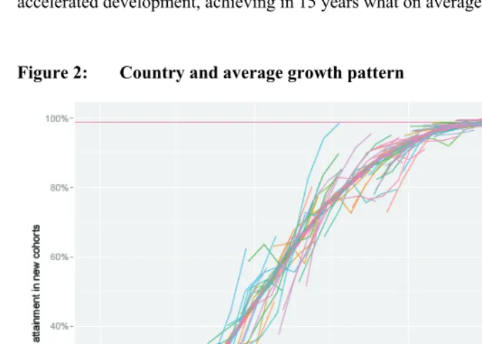
Both accelerating and decelerating phases of attainment expansion are found to be modeled well by cubic splines at all attainment levels. The placement of the point at which the curve switches from accelerating to decelerating expansion was chosen to ensure the splines connect smoothly. The exact placement is non-critical, since the curve is approximately linear for much of the central section. Fitting such bi-cubic models to each country shows good individual fits (in the vast majority of cases, with an adjusted R-squared greater than 0.8), and the resulting parameters, indicating the ‘pace’ with which different countries traverse the cubic curve, turn out to have a unimodal, fairly symmetric, and tightly clustered distribution. The parameter means across the individual country models may therefore reasonably be considered to constitute the ‘typical’ global trend. Countries that had already achieved 99% or higher participation were excluded in determining the overall mean expansion parameter. The projected trajectories resulting from applying these global trend parameters were examined for their plausibility.
in time and have equal weight. As a result, steeper trajectories are over-represented in terms of ‘ink’ on the graph. A plot of the relative slopes shows that the national trajectories are actually symmetrically distributed around the central trend. However, it is true that some countries have enjoyed much faster attainment growth than the central trend. As can be seen from the graph, the most successful countries have managed an accelerated development, achieving in 15 years what on average takes 65.
Figure 2: Country and average growth pattern
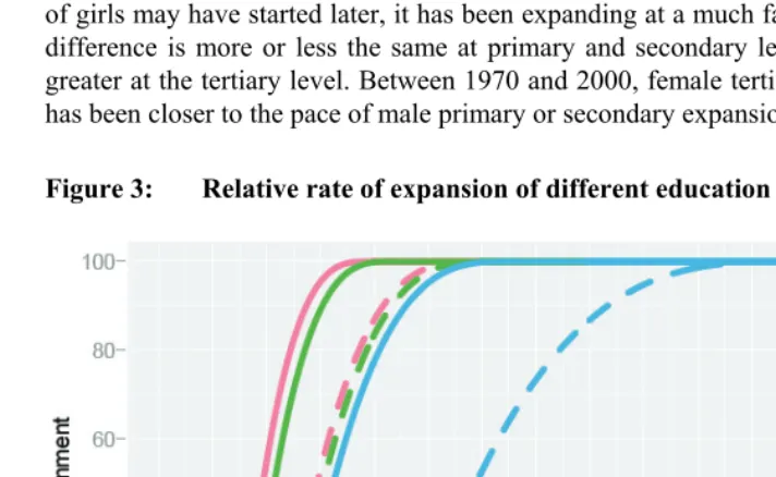
slower for the higher attainment levels. This is not a pre-specified constraint, but an empirical outcome of the model. Second, the parameters reflect the fact that, despite having started later and starting the study period at a lower level, female attainment has been growing more rapidly than male attainment, and is in the process of catching up.
The growth curves implied by these parameters are shown in Figure 3. Note that, for display purposes, the figure assumes that all phases start their expansion at the same time. In reality, different lags between schooling phases and attainment rates for males and females occur in different countries. Note also that the times indicated in the figure should be interpreted with caution, as they indicate the time required to reach true 100% starting from true zero. The model does not aim to fit the extreme tails, since in any case rounding occurs in actual statistical reports, and ‘universal’ schooling is generally considered to be achieved when 99%, or even 98%, is reached. Also, these are average times across stagnating and succeeding countries. What the comparison of the average growth patterns across phases and genders shows, however, is that, while the schooling of girls may have started later, it has been expanding at a much faster pace. The gender difference is more or less the same at primary and secondary levels, but dramatically greater at the tertiary level. Between 1970 and 2000, female tertiary attainment growth has been closer to the pace of male primary or secondary expansion in the past.
In this context, the different levels of confidence in the primary/secondary and tertiary growth patterns need to be noted. The first two are derived from past observations all along the growth curve. As such, it is fairly clear what the trend curve is, and it is reasonable to expect that countries at its lower end will move along it. With regard to tertiary expansion, however, the projection is a genuine extrapolation beyond levels currently observed, and should be treated more carefully.
The application of the GET scenario will normally result in more optimistic trajectories of educational attainment than either the CEN or CER scenarios. However, it is important to note that, in the case of the latter, this is not by definition. In the context of rapidly falling cohort sizes, the assumption of constant enrollment may in principle translate into increases in the proportions at higher attainment levels that are higher than the increases implied by the global education trend scenario. In fact, it could be argued that the GET scenario is rather conservative. The above parameters imply, for instance, that it takes a typical country about 40 years to raise female participation in primary schooling from 50% to 90%, and over 30 years after that to reach 99%. The latter in particular may seem discouragingly slow (moreover, female primary participation has been the fastest process over the period studied), but reflects the empirical average. While some countries have expanded access much more quickly, others have stagnated and made even less progress during the final decades of the 20th century, and this is reflected in the average slope.
5.2.4 The fast-track (FT) scenario
In addition to the above scenarios that define the lower bounds, or the worst case or ‘no change’ environments, an optimistic scenario has been defined. This is based on the GET scenario defined above, but assumes the achievement of certain milestones. If stated targets in attainment are not reached by certain years (both of which are defined below) under the assumptions of the GET scenario, then an accelerated rate of growth is applied that meets these targets.
Our fast-track scenario illustrates the implications of a new round of similar policy initiatives focusing on secondary education (the next logical step after the achievement of universal primary education). Since our category E3 is based on completed lower secondary, it is assumed that the target proportion will eventually be universal attainment of E3 by 2050. Since this target is very far off, however, a more achievable intermediate target is assumed for 2030. While no international policy frameworks have so far recommended specific targets for tertiary participation, the rapid pace of tertiary expansion in many parts of the world demonstrates a great amount of ambition in this regard, both individual and national. As an explicitly optimistic scenario, the achievement of a proportion of 60% at attainment level E4 is assumed to be reached by 2050. While this is as high as some of the very highest levels observed today, it is already exceeded by the aspirations of teenagers in some developing and transitional countries (OECD 2007). Even if the assumptions turn out to be over-optimistic (given that it appears increasingly unlikely that the EFA goals for enrollment will be achieved in 2015), the scenario will serve as a useful comparison with actual developments that can be helpful in assessing how much human capital has been ‘lost’ by missing the targets.
For the primary level (E2), the attainment of 99% transition to E2 by 2015 is assumed under the fast-track scenario, corresponding approximately to the achievement of the EFA goals. Lower secondary schooling (E3) is assumed to reach 50% of each cohort by 2030, and 90% by 2050. Tertiary (E4) is assumed to reach 60% by 2050.
5.3 A note on educational policy discontinuities since 1990
The back-projection dataset on which the global trend is estimated ends in the year 2000. Since the primary school attainment of 15-19-year-olds is considered, this indicator reflects primary intake ratios of 10 years before. Effectively, the data on the primary schooling of 15-19-year-olds up to the year 2000 reflects primary school experiences up to 1990. The year 1990 was, however, marked by the World Conference on Education For All in Jomtien, Thailand, at which the initial EFA goals were set. In the intervening years, a number of other international policy frameworks for educational development, including the MDGs and the FTI, were introduced.
The question therefore arises of whether, at the primary level, an extrapolation of trends prior to 1990 is misleading. It might be assumed that educational expansion has since accelerated as a result of the increased international attention. However, it is far from obvious to what extent this is actually the case.
educational attainment projections concern attainment levels, not enrollment, at the primary level there is a convenient near-equivalence between intake ratios and our attainment levels; since the transition from our level E1 to E2 is based on having received even a single year of primary schooling, the proportion in each year cohort in levels E2 and above is approximately equal to the intake ratio into primary school for that cohort.
The first difficulty arises from the need to match the single-year primary intake data with our five-year data. This is made more difficult by the fact that the intake statistics are not relative to a fixed age cohort, but are relative to the ‘official age of school entry’, which varies between countries, and is not given in the data. More serious, however, is the problem that, while the UNESCO statistics provide data on net intake ratios for children of the official school-entry age and those over or under the age by one year, in many cases a significant proportion of entrants appear to be more than one year over age. Using the gross intake ratio does not resolve these problems.
Unfortunately, the UNESCO data is far from complete for all countries in our database for the years 1991-2005. Concerns have also been raised about their consistency and reliability. Enrollment data are notoriously inflated. For these reasons, it was decided that primary intake statistics cannot be used to validate the continuity of the historical trend at this stage until their inconsistencies have been weeded out and the methodological issues resolved.
6. Results and discussion
6.1 Sample output
As an example of the kind of results obtained through the projection, Appendix B shows the full projection output for Pakistan, including age pyramids by education at various points in time and for the different education scenarios, as well as tabular output of the full age-sex-education population distribution in five-year intervals from the baseline year 2000 to 2050. The results for Pakistan clearly show the tremendous difference in the education level of the population between the different scenarios, and over time under the GET scenario.
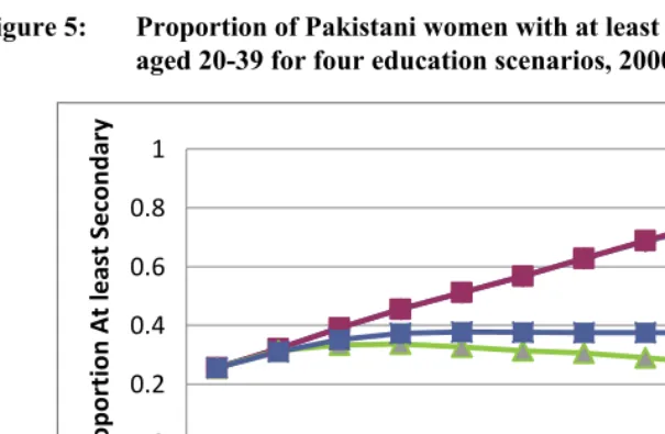
trends have on the education levels of future generations of mothers, and may serve as an input into estimates of future levels of child mortality and the level of literacy that future school children may be expected to be exposed to at home. The GET and FT scenarios are quite close, indicating that, in order to meet fairly ambitious targets, Pakistan would only need to follow a trajectory of expansion on secondary education participation that has many historical precedents, and can therefore be considered feasible. At the same time, the negative trend of the CEN scenario indicates that such a positive development is far from automatic, and requires considerable effort in terms of absolute expansion. Because of high population growth and momentum, constant school capacity would imply no improvement during 2000-2050, falling far short of what is achievable under the GET scenario. Figure 6 places the Pakistani projection under the GET scenario in the context of a number of other new IIASA member countries. Reflecting their similar starting position, India, and Pakistan share a similar projected trajectory. A second group is formed by Chile, China, and South Africa, all of which may reach near universal secondary attainment among women aged 20-39 by the end of the projection period.
Figure 4: Total fertility rate in Pakistan for four educational scenarios, 2000-2050 0 0.5 1 1.5 2 2.5 3 3.5 4 4.5 2000
‐2005
2005
‐2010
2010
‐2015
2015
‐2020
2020
‐2025
2025
‐2030
2030
‐2035
2035
‐2040
2040
‐2045
2045 ‐205 0 To tal Fe rt ilit y Rate
Figure 5: Proportion of Pakistani women with at least a secondary education aged 20-39 for four education scenarios, 2000-2050
0 0.2 0.4 0.6 0.8 1
2000 2005 2010 2015 2020 2025 2030 2035 2040 2045 2050
P
roporti
on
At
le
as
t
Se
conda
ry
GET FT CEN CER
Figure 6: Proportion of women with at least a secondary education aged 20-39 for the global education trend scenario, selected countries, 2000-2050
0 0.2 0.4 0.6 0.8 1 1.2
2000 2005 2010 2015 2020 2025 2030 2035 2040 2045 2050
P
ro
p
orti
on
at
le
as
t
se
conda
ry
Republic of Korea Chile
China South Africa