of peer-reviewed research and commentary in the population sciences published by the Max Planck Institute for Demographic Research Konrad-Zuse Str. 1, D-18057 Rostock · GERMANY www.demographic-research.org
DEMOGRAPHIC RESEARCH
www.demographic-research.org
VOLUME 13, ARTICLE 1, PAGES 1-34
PUBLISHED 15 JULY 2005
http://www.demographic-research.org/Volumes/Vol13/1/ DOI: 10.4054/DemRes.2005.13.1
Research Article
Placing the poor while keeping the rich in their
place:
Separating strategies for optimally managing
residential mobility and assimilation
Jonathan P. Caulkins
Gustav Feichtinger
Dieter Grass
Michael Johnson
Gernot Tragler
Yuri Yegorov
1 Introduction 1
2 Policy context 3
3 The model 6
4 Qualitative analysis 9
4.1 Derivation of the canonical system 9
4.2 Isoclines and steady states 10
4.3 Critical line and lens 11
4.4 Limitations of the qualitative analysis 11
5 Choice of parameters 11
5.1 Housing market adjustment speed coefficient, α 11
5.2 Assimilation coefficient, γ 12
5.3 Flight coefficient, β 12
5.4 Objective function coefficient for X, ρ 13
5.5 Quadratic cost coefficient, c 14
5.6 Discount rate, r 14
5.7 Summary of parameter values 14
6 Results of numerical simulations 15
6.1 Economic meaning of different equilibria 15
6.2 Basecase results 16
6.3 Sensitivity with respect to flight parameter β 18
6.4 Sensitivity with respect to parameter α 21
6.5 Bifurcation diagram in α – X space 26 6.6 Summary of sensitivity with respect to interactions between α and c 27 7 Conclusions and policy implications 28
8 Acknowledgements 30
Placing the poor while keeping the rich in their place:
separating strategies for optimally managing residential mobility and
assimilation
Jonathan P. Caulkins1, Gustav Feichtinger2, Dieter Grass3,
Michael Johnson4, Gernot Tragler5, Yuri Yegorov6
Abstract
A central objective of modern US housing policy is deconcentrating poverty through “housing mobility programs” that move poor families into middle class neighborhoods. Pursuing these policies too aggressively risks inducing middle class flight, but being too cautious squanders the opportunity to help more poor families. This paper presents a stylized dynamic optimization model that captures this tension. With base-case parame-ter values, cost considerations limit mobility programs before flight becomes excessive. However, for modest departures reflecting stronger flight tendencies and/or weaker des-tination neighborhoods, other outcomes emerge. In particular, we find state-dependence and multiple equilibria, including both de-populated and oversized outcomes. For certain sets of parameters there exists a Skiba point that separates initial conditions for which the optimal strategy leads to substantial flight and depopulation from those for which the op-timal strategy retains or even expands the middle class population. These results suggest the value of estimating middle-class neighborhoods’ “carrying capacity” for absorbing mobility program placements and further modeling of dynamic response.
1Carnegie Mellon University, H. John Heinz III School of Public Policy and Management, 5000 Forbes Ave.,
Pittsburgh, PA 15213, USA, E-mail: [email protected]
2Vienna University of Technology, Institute for Mathematical Methods in Economics, E-mail:
3Vienna University of Technology, Institute for Mathematical Methods in Economics, E-mail:
4Carnegie Mellon University, H. John Heinz III School of Public Policy and Management, 5000 Forbes Ave.,
Pittsburgh, PA 15213, USA, E-mail: [email protected]
5Vienna University of Technology, Institute for Mathematical Methods in Economics, E-mail:
1. Introduction
This paper addresses the dynamic optimization problem faced by a social planner who wants to integrate a stream of poor families into an existing middle-class neighborhood without inducing “middle-class flight”. Attempting to place “too many” poor families too quickly could induce current residents to relocate and/or deter affluent residents of other communities from moving in, both of which could reduce the tax base of the communi-ties to which poor families relocate. On the other hand, placing too few poor families squanders the opportunity to use the resources of the community to help assimilate poor families into the middle class.
The model is highly stylized but is inspired by a pressing practical problem. The United States has pockets of concentrated poverty in most of its major cities and some adjoining older suburbs. Upward social mobility from these neighborhoods is limited, creating a persistent “underclass” of the “truly disadvantaged” (Wilson 1987). Some of these neighborhoods contain publicly-subsidized housing developments. Over the last ten years the government has pursued an active policy of “de-concentrating” poverty by subsidizing movement of tenants from high-poverty, racially segregated communities into more affluent neighborhoods using “housing mobility programs” such as the nationwide Moving to Opportunity (MTO) experiment (U.S. Department of Housing and Urban De-velopment 1999). The underlying premise, for which there is considerable empirical support, is that poor families can do better on a variety of social, health, education, and economic indicators if they have the opportunity to choose good-quality housing in more-affluent destination communities (Johnson, Ladd, and Ludwig 2001).
The model is formulated as an optimal dynamic control problem. This is a natural framework for reflecting the dynamic, endogenous response of current residents to an inflow of poor residents, but to the best of our knowledge this methodology has rarely been used to study housing issues and is not used very frequently in demographic research more generally. Note: city growth is not the only domain of interest to demographers that invites dynamic models with growth under externalities. Another example would be ecological models where both the flow of agricultural products and the stock of wild nature bring utility.
This dynamic approach generates interesting insights. For example, the model dis-plays “tipping” – the phenomena studied extensively by Schelling (1973) of having mul-tiple stable equilibria surrounded by neighborhoods of attraction and unstable equilibria, although in this case this characterization pertains to trajectories observed when the so-cially optimal policy is pursued, not the uncontrolled dynamics.
with little tolerance to each other. In this case, economic class. Unlike Schelling’s and other traditional models, ours explicitly includes two types of externalities: (1) negative externalities generated by poor families and which are of private concern to the middle-class and (2) positive externalities generated by middle middle-class families and which are of interest to the social planner at least in part because of their effect on the population dy-namics. On the other hand, Schelling’s model relied on a spatial concept of neighborhood, whereas we abstract from an explicit grid representation of neighborhood location.
As so often occurs, bringing new methods to a problem domain generates results that are interesting from the methodological perspective. In this case we find a one-state model with two so-called DNS thresholds and a “lens” that focuses candidate solution trajectories in a way that lets them pass through a singularity. Mathematical properties of the lens are explored by Caulkins et al. (2004), who primarily consider a simpler version of this model (one without assimilation) and for more arbitrary parameter values. Here we simply use those properties when establishing what are the optimal solutions; readers are referred to the earlier paper for derivation of those properties.
Paper structure. In Section 2 we elaborate on the policy context examined. Section 3 introduces the formal assumptions and formulation of the mathematical model, while Section 4 provides its qualitative analysis. In Section 5 we discuss what are realistic parameter values for the model. Section 6 describes the results of numerical simulations and comparative statics, that often reveal structural changes. It is a core part of the paper, since many policy issues are also discussed here, as well as bifurcation diagrams and other simulation results. The paper ends with conclusions and policy implications.
2. Policy context
The recent emphasis on integrating low-income families into middle-class neighborhoods represents a substantial shift in housing policy. Public housing in the US was originally largely a product of the Great Depression and immediate post World-War II era. The emphasis was on increasing the supply of affordable housing by building geographically concentrated projects run by public housing authorities (PHAs). Much of the country was racially segregated at the time, and PHAs were no different. As Popkin, Rosenbaum, and Meaden (1993, p. 179) note, “Over several generations, many public housing authori-ties established and perpetuated racially segregated and discriminatory systems for public housing and other housing assistance, in violation of fair housing laws.”
versa, e.g., because the vast majority of current residents and of people seeking public housing were minority or because members of one group refused offers of placement in facilities where they would be in the minority. Indeed in a series of Texas court cases known collectively as the Young case it was ruled that massive and mandatory transfer of tenants within public housing should not be seen as the primary remedy.
An alternative strategy was pioneered in the settlement to the Gautreaux class-action suit originally filed in Chicago in 1966. That settlement sought to remediate past discrim-ination by moving low-income African-Americans to white areas via “Section 8” certifi-cates and vouchers that subsidized the rent tenants paid to private landlords in “scattered site housing” instead of placing them in other PHA projects.
Evaluations of the Gautreaux experiment found that participants who moved to sub-urban communities enjoyed better educational and labor market outcomes than did par-ticipants who moved to neighborhoods within the central city (Popkin, Rosenbaum, and Meaden 1993, Rosenbaum 1995). These results came to light at a time when a consensus was emerging in the social science literature that neighborhood attributes influence a vari-ety of economic, health, and criminal behaviors, and that the proportion of neighborhood households with incomes below the poverty line is a particularly important attribute (e.g., Mayer and Jencks 1989, Massey, Gross, and Eggers 1991, Turner and Gould Ellen 1997). In light of these developments, the Clinton Administration broke with the past policy of contesting the lawsuits and fundamentally changed the goal of federal housing pol-icy from supplying housing units to expanding opportunities for tenants to live in high-quality, desegregated neighborhoods, both by converting traditional housing projects into mixed-income residential developments (so-called “HOPE VI” revitalizations) and by ag-gressively using vouchers to place tenants in privately-owned scattered site housing.
and white, with evidence of one minority group fleeing from another (Fairlie 2002) and middle-class minorities fleeing from poor minorities (Winsberg 1985, Murphy 1995). Fi-nally, residential segregation by race has been falling – albeit very slowly – in the US since 1970, but economic segregation within race has been rising, particularly for minori-ties (Jargowsky 1996).
A central concern with government interventions designed to place poor families in middle-class neighborhoods is the possibility of adverse economic impact on the neigh-borhood, e.g., through declining property values (Galster, Tatian, and Smith 1999, San-tiago, Galster, and Tatian 2001) or triggering a downward economic spiral if long-time residents move away (“middle-class flight” or “white flight” in the racial integration con-text). There is a large literature on “flight” that debates many things such as whether the primary driver is increased egress or normal turnover coupled with lack of replacement (c.f., Galster 1998, Gould Ellen 2000), but with some exceptions concerning particular issues (e.g., Freeman and Rohe 2000), the consensus is that flight still occurs and is an important issue (Clotfelter 2001).
Clearly if the principal policy objective is to integrate poor families into middle-class neighborhoods, that objective is undermined if there is a large net exodus of middle-class neighbors. Hence, we view the policy planner’s objective with respect to a given neighborhood as two-fold: place there as many poor families as possible while simulta-neously maximizing the number of middle-class residents. This dual-objective is broader than some in the literature, which focus exclusively on outcomes for the PHA/Section 8 tenants, although it still neglects outcomes for poor families “left behind” in the neighbor-hoods from which the MTO families come (cf., Johnson and Hurter 2000). This exclusion can be partially justified on grounds of tractability, lack of basis for estimating outcomes for those left behind, and the parochial interests of municipal policy makers when the movement from poor to middle-class neighborhoods crosses local jurisdictional bound-aries.
in some respects and a disadvantage in other respects. Manski (1993) elaborates on why the econometric identification problems limit the inferences that can reliably be drawn from the empirical record. Furthermore, De Souza Briggs (2003) notes there is some-thing of a choice between “cure” strategies that try to reduce segregation and “mitigate” strategies that seek to reduce the social costs of segregation without actually changing where people are willing and able to reside.
In this paper we take no position concerning whether integrating poor families into middle-class neighborhoods is the right overall strategy. Rather, given that overall policy directive, we explore the fundamental management question: how best could such a strat-egy be implemented?
3. The model
The model presented here was first introduced by Caulkins et al. (2004). It is highly stylized, and many considerations are suppressed in the interest of framing an essential dynamic of the problem in a novel way.
The key measure of the health of the neighborhood is taken to be the number of middle-class families who live there at timet, denoted by the state variableX(t). The key policy variable is the rate at which poor families are placed in the neighborhood, denoted by the control variableu(t).
7
The number of middle-class families, X, varies over time due to three influences. First, there are the underlying natural or “uncontrolled” dynamics that would pertain even if there were no MTO policy intervention (i.e.,u=0). In many respects, housing markets operate like other economic markets, with price adjusting to balance supply and demand. For simplicity we imagine the neighborhood is an established, fully-developed area so the housing stock is fixed at a size that would under normal circumstances support some given population (without loss of generality normalized to be unity). If the resident population falls below that level, presumably local prices would decline, attracting immigration from other, comparable middle-class neighborhoods. Conversely, if the neighborhood popula-tion grew beyond its normal level (X > 1), residents would flow to other middle-class neighborhoods that were less congested. Realistically, the neighborhood’s normal popu-lation density depends on the surrounding city’s overall growth trajectory. If the city were booming, the neighborhood’s normal population density would increase over time. Con-versely if the population base were eroding. We abstract from such considerations and imagine that the normal population for this neighborhood is constant over time. There
7Note that the time argument
does not appear to be a definitive, standard model in the literature for describing these nat-ural adjustment processes. Hence, for convenience we adopt the familiar logistic growth curve.
The second factor influencing changes in the stock of middle-class residents is “middle-class flight” (and/or “middle-“middle-class avoidance”) induced by the placement of poor families in the neighborhood. Again there does not appear to be a standard functional form in the literature, in part because the reality is rather more complicated than what can be captured in a one-state model. For example, Galster (1998) finds that racial transition depends not only on racial composition in the immediate neighborhood, but also on proximity to other majority minority areas, attitudes, and affirmative marketing strategies. Likewise, a one-state model cannot reflect details of the spatial distribution (DeMarco and Galster 1993). Also, flight may be driven not only by immigration into the residential neighborhood but rather by immigration of children into the school district (e.g., Clotfelter 2001, Fairlie 2002). Perhaps not surprisingly some subgroups appear more likely to flee than others. E.g., Gould Ellen (2000) argues that homeowners are more likely to leave than are renters and that families with children are more likely to flee than families without children, par-ticularly if the children attend public schools.
One central question is whether flight is driven more by the current inflow of poor immigrants or by their accumulation over time, perhaps relative to the size of the stock of middle-class families. On that point, there seems to be some reason to believe it is the current inflow. E.g., Gould Ellen (2000, p. 686) argues that “whites do not appear to care very much about the proportion of a neighborhood that is African-American, [but] whites do tend to avoid neighborhoods in which the proportion of families who are African-American is increasing (independent of the current size of the minority population)”. Again we opt for the benefits of simplicity and assume that middle-class flight is simply proportional to the rate of inflow of poor families. This is akin to the finding of Betts and Fairlie (2003) in the context of native-born and immigrant populations that “For every four immigrants who arrive in public high schools, it is estimated that one native student switches to a private school.”
Presumably the number of poor people assimilating is increasing both in the number who are placed and, hence, are candidates for assimilation (i.e., is increasing inu) and also in the number of middle-class neighbors (X). Again, the literature does not offer guidance as to what functional forms might be preferred. At the suggestion of Rosser, we opt for a simple bi-linear relationship: assimilation is proportional to the product ofuand
X.
One potentially awkward aspect of this simple form is that if X is large enough, the proportionality constanttimesX may exceed 1, implying that the number of poor people being assimilated can exceed the number of poor people being placed there by the policy maker through the housing subsidy program. That is by no means implausible since poor people in the program might attract other people to enter the neighborhood who are not part of the formal program and, hence, do not have their flow enter the cost-function and are not so visible as to affect out-migration. E.g., residents might be very conscious of poor people placed by a formal public program, but their friends who just move in on their own may not be noticed and, hence, might not engender the same amount of middle-class flight. Nevertheless, it will be important to remember this interpretation when the analysis suggests the optimal solution hasX>1.
The other great simplification of assimilation in this model stems directly from having only a single state variable to represent the neighborhood’s current population. As a result, newly placed poor families either assimilate immediately or depart. There are not additional states that explicitly model the gradual process by which a family remaining in the neighborhood moves up the socio-economic ladder over time. Elaborating on that dimension would be an important extension for further research.
Together these consideration suggest the dynamic state equation:
_
X =aX(1 X) u+Xu; (1)
wherea; and are positive constants governing, respectively, the speed with which the equilibrium population is approached, the extent of middle-class flight, and the rate of assimilation of poor families into the middle class. Note that families that are not assimilated play no further role in the state dynamics because there is not a second state variable to track poor people living in the neighborhood. Practically speaking, those that do not assimilate might well leave the community, particularly after their eligibility for tenant-based housing subsidies expires and they would have to pay full market rates for housing.
To complete the formulation we must specify an objective function. We adopt the fa-miliar perspective of maximizing the infinite-horizon, discounted net social benefit.8The
8Note that we assume an infinite planning horizon for reasons of analytical tractability. For instance, this
review of the policy context above justifies counting both placing poor families (u) and maintaining middle-class residents (X) as socially beneficial. Without loss of generality, we scale the benefit function so the coefficient onuis unity and letdenote the relative benefit per unit time ofX compared withu.
Finally, we presume that the policy intervention itself carries some cost, including administrative costs, costs of counseling families concerning their initial placement and follow up, property value impacts, and deadweight losses associated with constraining choices. We presume for the standard diminishing returns arguments that these costs are convex. Again in the absence of evidence favoring one specific functional form over another, we opt for simplicity and use a quadratic form. The linear term is subsumed into the (scaled) coefficient onu, leaving only the squared term to appear independently in the objective function.
Hence, the dynamic optimization problem we wish to analyze can be written:
max fu(t)0g Z 1 0 e rt (u(t) cu 2
(t)+X(t))dt;
s:t: _
X(t)=aX(t)(1 X(t)) u(t)+X(t)u(t); (2)
whereris the time discount rate andcis the program cost coefficient.
It should be clear to the reader that this is a highly stylized model not only in its structural simplicity (e.g., using a single state variable to represent the neighborhood’s resident population) but also in terms of the functional forms employed, none of which have been validated in any sense of the word. Hence, we focus on qualitative insights, not specific numerical results and view this entire paper as somewhat exploratory.
4. Qualitative analysis
4.1 Derivation of the canonical system
The analysis proceeds in the usual manner for an optimal dynamic control problem (cf., Chiang 1992, Feichtinger and Hartl 1986). The current value Hamiltonian, denoted by
H,
H =(u cu 2
+X)+[aX(1 X) u+Xu]; (3)
leads to the following set of first order conditions:
_
X =aX(1 X) u+Xu; (4)
_
=(r a(1 2X) u) ; (5)
H u
where the Hamiltonian maximizing condition (6) must hold for interior solutions.9
If we exclude, then our system can be written in theX uspace:
_
X=aX(1 X) u+Xu; (7)
_ u=
(1 2cu)
2c( X)
[aX(1 X) u+Xu]+
1 2cu
2c
[a 2aX+u r]+
2c
( X): (8)
4.2 Isoclines and steady states
We start the analysis by locating the steady states of the canonical system. The first isocline, _
X=0, leads to the equation
u(X)=
aX(1 X)
X
: (9)
It always has two roots (i.e.,X = 0 andX = 1) and a vertical asymptote at X =
X
;X
=, separating two branches of this curve. The general shape depends on the value of the critical parameterX
. IfX
<1, both branches have positive slope, and while crossingX
the value ofuchanges from+1to 1. IfX
>1, the left branch has an inverse-U shape, while the right branch isU-shaped.
The second isocline,u_ =0, has a more complicated form, but some qualitative in-sights can still be gained. First of all, it has a singularity in the pointX =X
. Hence, the vertical lineX = = marks the border between two zones, where the vector field is continuous. This singularity is broken only in one point, which belongs to the isocline itself. The intersection between the isoclineu_ =0and the singular lineX =X
takes place at(X==X
;u=1=(2c)u
). This point (which we will call the critical
point) has an important role, and its properties will be elaborated below.
The points of intersection between the isoclines give us candidates for equilibria. Note that at all points satisfying _
X =0, the expression foru_ =0simplifies considerably, so we can solve for
X(u)=
(1 2cu)(a r+u)+
2a(1 2cu)+
; (10)
which can be studied together with the equationu(X)derived above. In the asymptotical casec!0,X(u)=c
1 +c
2
u+O(c), wherec 2
==(2a+)>0. Such a positively
9Since
H uu
sloped curve in many cases will have at least two intersections withu(X). Thus, gener-ically we have multiple equilibria. Havingc >0makes the curveX(u)nonlinear, and this can increase the number of equilibria. Further analysis can be done using numerical methods. For analytical results and the special case of no-assimilation (i.e., =0) see Caulkins et al. (2004).
4.3 Critical line and lens
Before proceeding with the analysis of the case>0, we need to address one mathemat-ical oddity. Typmathemat-ically when solving dynammathemat-ical systems, if there is more than one saddle point, then those saddle points are separated by some unstable equilibria. However, it turns out that for many parameter values, we find forX >0three saddle points but just one unstable equilibrium. Obviously in a one-state model, one unstable equilibrium can’t separate all pairs of saddle points. It turns out that in this model the critical point behaves in a rather interesting and unusual way. It is not a steady state, but it acts like an unstable equilibrium in the sense of separating successive saddle point equilibria.
The properties of this critical point are explored by Caulkins et al. (2004) who show that a finite measure of trajectories can pass between two semiplanes separated by a sin-gular border. They converge in a lens formed by the critical point, and then diverge. If
X
<1, these trajectories pass through the lens from left to right; ifX
>1they move from right to left. These observations solve the paradox about the coexistence of one un-stable node with three saddles and helps us to determine which dynamic trajectories are candidates for optimal solutions.
4.4 Limitations of the qualitative analysis
Except for the special case =0the underlying problem is too hard to address analyti-cally. That special case of no assimilation is investigated by Caulkins et al. (2004). Here we pursue the more realistic and complicated case for>0numerically. To do so, it is important to give some thought to appropriate ranges for the parameter values, which is the content of the following section.
5. Choice of parameters
5.1 Housing market adjustment speed coefficient,a
The uncontrolled dynamics are _
uncon-trolled equilibrium. That is, how long, on average, does it take for a house to sell in a healthy middle-class neighborhood (Xclose to 1)?
Over the last 15 years, the average for a new home has been between 3:6and6:9 months (U.S. Census Bureau 2004a). The average of those averages is4:89, suggesting
a=(12=4:89)ln(2)=1:7, which we round up to a base case of 2.
However, the American Housing Survey 2001 (AHS) (U.S. Census Bureau 2004b) in-dicates that there is considerable variation in time spent on the market, and lower values of parameteracan yield qualitatively different results, so we also explore the consequences of introducing housing mobility programs to neighborhoods with weaker real estate mar-kets. The AHS data indicate that13:4%of units were on the market for more than 2 years. The data are reported in categories, so we do not know exactly what vacancy period is the 90th percentile. It is clearly above 24 months and might be on the order of 36 months (a=0:231). For a round number we takea=0:2(vacancy period 41.6 months) because that is our base case value (a=2) divided by 10.
5.2 Assimilation coefficient,
The parameterreflects the “success” or “assimilation” rate for persons who participate in housing mobility programs, i.e. the proportion of families initially placed in low-poverty or low-percent minority (what we call “middle-class”) neighborhood who stay for an extended period of time.
The MTO Interim Impacts Evaluation (U.S. Department of Housing and Urban De-velopment 2003) reports that35%of all “experimental group” families who successfully found rental housing between 1994 and 1998 were recorded in 2002 as living in Census tracts with Census 2000 poverty rates of20%or less. Also for MTO, Shroder (2001) reports that64%of treatment group started on welfare. Thirteen quarters later it fell to
34%, suggesting an assimilation rates of1-34=64=47%.
DeLuca and Rosenbaum (2003) concluded that for the Gautreaux program, after an average of 17 years post-move, about57%of suburban movers remain in the suburbs. Also, about37%of participants who moved to neighborhoods that were15%black or less initially remain in neighborhoods that are30%black or less. This would imply a success rate for the Gautreaux Program of between37%and57%.
Given these three figures (37%;47%;57%), we set=45%in our base case.
5.3 Flight coefficient,
from lower-class could be stronger than flight from immigrants, suggesting somewhat larger values ofin our context.
Gould Ellen (2000, p. 124) reports that “The probability of the typical white home-owner moving is between 2:0and3:5 percentage points higher when the black popu-lation has grown by 10 percentage points over the decade.” For a neighborhood around the uncontrolled steady state, an increase of10%over the decade meansu=0:01. If that inflow leads to a0:02to0:035increase in the per capita outflow rate, that means
u=0:02-0:035and, hence,=2-3:5. Given=0:45, that impliesin the range of0:9-1:575.
In light of this, we take=0:5as our base case, but also consider sensitivity excur-sions with smaller (=0:25) and larger (=1:0or1:5) values.
5.4 Objective function coefficient forX,
Recall thatis the value per middle class family per year relative to the value per low-income family placed, so first we need the value per low-low-income family placed. The ONDCP (2002, Table 13) is a federal government agency that offers an estimate of the monetary value of saving a high-risk youth, based on the work by Cohen (1998). Interpo-lating for a5%discount rate, the values would be $1:1-1:6M.
Shroder (2001) reports that for kids in MTO treatment vs. control: (1)21%vs. 35% had trouble with teachers, (2)21%vs. 32%were disobedient at home, (3)5%vs. 19% were “mean or cruel to others”, and (4)16%vs.28%were “unhappy, sad, or depressed”. These short-term findings might suggest that about12%of kids will be “saved”, but gains can erode over time. The MTO experiment is too recent for there to be long-run results, but Caulkins et al. (2002) found that, in the context of drug prevention, long-term gains were about one-fifth of short-term gains in percentage terms. So assuming an average of 2:5kids per family, the social benefit per family placed might be something on the order of$1:1M-1:6M12%2:520%=$66;000-$96;000, or an average of about
$80;000.
The average cost per family placed is roughly the $70M Congress appropriated di-vided by 2414 households = $29;000per household placed, or a net benefit of $80;000
$29;000or about $50;000.
5.5 Quadratic cost coefficient,c
There is currently no empirical basis for estimating parameterc. The inflowuin the five MTO cities was about0:24per1;000current residents oru=0:0002. That is so small that thecu
2
term is negligible and, indeed, there is no discernable relationship between costs per person placed and placement intensity across the five cities.
Hence, what value of parametercmakes sense is best thought of by reference to the instantaneous part of the objective function pertaining to the control:u cu
2
. This says that, leaving aside theX term, the instantaneous satisfaction the policy maker derives is maximized whenu=1=(2c)and is driven to zero ifu=1=c. In other words, when focusing only on short-run considerations, the convex program costs make the preferred rate of poverty de-concentration in the short runu=1=(2c)and by the timeu=1=cthey would offset all of the poverty de-concentration benefits. A value ofc=20implies that these rates are placing one poor family per 40 middle class families per year and one poor family per 20 middle class families per year, respectively. At one level these seem about right. The first might be a good target; the second might be overly aggressive. However, those judgments are probably tempered by long-run considerations including flight and assimilation. Focusing only on the short-run considerations driven by the convexity of the program cost structure, the optimal and maximum desirable placement rates might be higher, so we also consider examples below with lower values of the parameter c, specificallyc=2. Given the lack of empirical basis, we viewc=20andc=2as both being in some sense base case values, rather than arbitrarily anointingc =20as the best guess and viewingc=2as merely a sensitivity excursion.
5.6 Discount rate,r
The annual social planner discount rate is customarily between3%and7%. We take as our base valuer=0:05.
5.7 Summary of parameter values
Table 1 summarizes the parameter values used in numerical experiments. In this paper we maintain the values ofr =0:05,=0:02and =0:45, but allow parametersa;cand
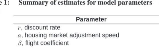
Table 1: Summary of estimates for model parameters
Parameter Base Case
r, discount rate 0.05
a, housing market adjustment speed 2
, flight coefficient 0.5
, assimilation coefficient 0.45
, objective function coefficient on middle class state 0.02
c, program cost coefficient 2 and 20
6. Results of numerical simulations
6.1 Economic meaning of different equilibria
Numerical simulations reveal the existence of up to three saddle point equilibria of differ-ent types. To understand them intuitively, it is useful to contrast them with what happens when there is no inflow of poor families. In that case, the model reduces to the logis-tic equation _
X = aX(1 X), which has unstable and stable steady states at X = 0 andX = 1, respectively. The second dominates because for any positive initial state (X(0) > 0), the trajectories always converge to this natural or uncontrolled size of the neighborhood (X =1).
With a mobility program (u > 0), two other factors in addition to own growth (aX(1 X)) influence the dynamics ofX, namely flight due to immigration ( u) and assimilation of immigrants (Xu).
10 The relative and absolute magnitudes of these
three flows differ in the three types of saddle point equilibria.
In the first type of equilibrium, the stateX is substantially below the natural level 1, undermining assimilation. In such equilibria, it is growth via the logistic term (in-migration of families attracted by a relatively abundant housing stock) that is primarily responsible for off-setting mobility program-induced middle-class flight. In the case when the equilibriumX is small enough that the natural logistic growth term (aX(1 X)) is small, thenumust be quite small as well. This is a relatively unhealthy community, but it could still be optimal to pursue a policy that creates such a community if the decision maker is relatively short-sighted (rlarge) and values highly program placements relative to other considerations (andcsmall). Such equilibria might be called “smallX, modest
uequilibria.”
Another type of equilibrium with u > 0 is close to the uncontrolled equilibrium (X near 1). At this point the natural population growth is small (logistic term is close
10The functional form of the assimilation term was proposed to the authors by Barkley Rosser (personal
to0), and the typically modest inflow of poor families (usmall to moderate) generates assimilation and flight to roughly equal degrees, leaving the middle-class population very near its normal level in the absence of a control (X close to 1). In such an equilibrium, the poverty de-concentration program does not dramatically alter the character of the neighborhood, and we might call it a “lowu, averageX equilibrium.”
In the third type of equilibrium the neighborhood is densely populated (X >1), so not only program-induced middle-class flight but also the natural population dynamics tend to reduceX. Assimilation is the only factor tending to increaseXand preserve the high population density. Due to the assumption that assimilation is proportional to the level ofX, a high proportion of the fairly large inflow of poor families,u, is assimilated. However, even the middle-class residents are relatively transient, leaving at high rates. Such equilibria might be called “highX, highu” equilibria, and be thought of as akin to the transition neighborhoods in New York City that assimilate foreign immigrants.
Depending on the parameter values, 1, 2, or all 3 equilibria may exist as saddle point solutions to the canonical system. In some sense the policy questions in this model boil down to: for any given initial neighborhood, under what conditions is it optimal to ap-proach each of these three types of neighborhoods and through what immigration “trajec-tory”u?
6.2 Basecase results
With base case parameter values, there are saddles corresponding to all three equilib-ria. There is a vortex between the first two, and the lens separates the second and third. However, the middle saddle, withX = 0:9994, dominates. That means, regardless of the initial state, it is always optimal to converge to a standard middle class neighborhood with mobility programs run at such a modest rate that they have minimal impact on the neighborhood.11
That the third saddle can never be a long-run optimum follows directly from the prop-erties of the lens sketched above. Since the flow lines all pass from right to left, all trajec-tories starting with largeXpass through the lens from right to left and must approach a long-run equilibrium that is to the left of the lens.
That the smallX equilibrium can never be optimal requires a numerical proof anal-ogous to that given in Caulkins et al. (2004). Intuitively, the essence of the proof is that the trajectories approaching the smallest saddle point all involve using mobility programs at levels withu> 1=2c, which does not make economic sense. (With such highu, the short-term costs of the mobility program undercut even its short-run benefits. Further-more, there is rapid erosion of the middle-class population due to flight, and the shadow
value of the middle class population is always positive.)
Ifc were smaller, then 1=2c would be larger, so given the uncertainty concerning the quadratic cost coefficientc(see above), this suggests examining results for a smaller
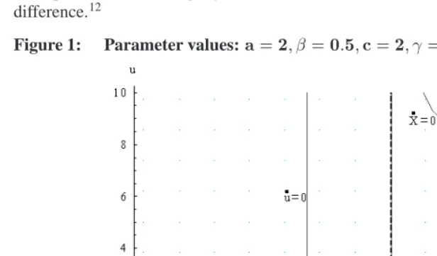
c = 2, notc = 20:The resulting phase portrait (Fig. 1) is topologically identical. (It, rather than the portrait with c = 20is shown because it is easier to read.) The long-run equilibrium shifts slightly fromX =0:9994to 0.99333, but otherwise there is little difference.12
Figure 1: Parameter values:a=2;=0:5;c=2;=0:45;r=0:05;=0:02
Note: The saddleX=0:993is optimal. Saddle paths from both left and right are shown; they almost
coincide withu= 1 2c
. The steady states representing small and large cities are suboptimal.
In the following subsections we deal with sensitivity analyses for different parameters. For a better understanding of how the different cases discussed are interrelated, we pro-vide a “road-map” in Fig. 2. This “road-map” shows interrelations between all considered cases, marked as corresponding figures with particular parameter values.
12Clearly, the corresponding
ugrows approximately by factor 10, fromu=0:0249tou=0:249, always
Figure 2: “Road-map” showing the link between different cases investigated
Fig. 8
a=0:05
=0:5
c=2
Skiba
Fig. 7
a=0:04
=0:5
c=20
Weak Skiba
Fig. 6
a=0:2
=0:5
c=20
Fig. 3
a=2
=0:25
c=2
Fig. 1
a=2
=0:5
c=2
Fig. 5
a=2
=1:5
c=2
Fig. 4
a=2
=1:5
c=20
Fig. 0
(case not shown)
a=2 =0:5
c=20 ? - ? ? ?
c=2 c=20
Note: In all cases,=0:45;r=0:05;=0:02. We start from two baseline cases: Fig. 0 (c=20) and
Fig. 1 (c=2). In both cases,a=2and=0:5. From there we continue by changing parameter, which
also can take the values0:25(Fig. 3) and1:5(Figs. 4 and 5). Note that Figs. 4 and 5 differ only in the value of
c. Three figures at the bottom line have different values for parametera. In the cases of very low a (Figs. 7 and
8) we have Skiba points.
6.3 Sensitivity with respect to flight parameter
Mathematically, decreasing the amount of middle-class flight by reducingfrom0:5to
0:25changes the picture considerably. Now the lens separates the first two saddle points, passing the flow from left to right. The smallX equilibrium cannot be optimal due to a theorem that says that the objective function value for a given level of the state variable is increasing in the distance to the _
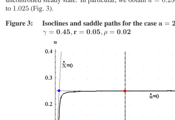
long-run equilibrium. That is, this reduction in the flight parameter only reinforces the strength of the middle-type saddle. Substantively, the only consequence is that this greater strength allows the mobility programs to increase the population to slightly more than its uncontrolled steady state. In particular, we obtainu=0:2505andX shifts from0:9933 to1:025(Fig. 3).
Figure 3: Isoclines and saddle paths for the casea=2;=0:25;c=2;
=0:45;r=0:05;=0:02
Note: The critical line is shown as dashed. There are 2 saddles, and the right (close toX=1) is optimal.
Increasing the amount of middle-class flight by increasingfrom0:5to1:0withc=
20not only does not change the solution much, merely shifting the long-run equilibrium from (X = 0:9994;u = 0:0249) to(X = 0:9930;u = 0:0248), it also leaves the topological structure intact.13 Even increasing
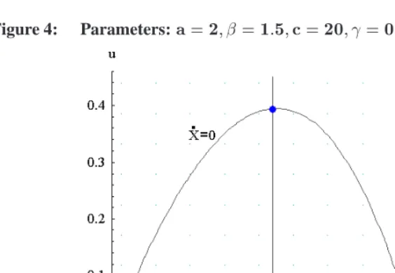
to1:5(Fig. 4) just pushes the long-run equilibrium (middle-size city) down a little further, to(X=0:986;u=0:0247).
However, if the mobility program is cheaper (c=2) and flight is greater ( =1:5), the combined effects move the long-run equilibrium more substantially, down toX near
0:834instead of close to1:0(Fig. 5).
13Increasing
makes theuat the unstable node smaller and at the same time leads to an increase of theX
Figure 4: Parameters:a=2;=1:5;c=20;=0:45;r=0:05;=0:02
Note: The middle-size city (X=0:986) always dominates. Small (X=0:02) and oversized city
(X=6:1, not shown) are never optimal. The fourth equilibrium (X=0:53) is a vortex.
As one can see from Fig. 5, the vortex has dropped substantially (lower value ofu), approaching the levels of those for the saddle points. While at this point the equilibrium withX near 1 continues to dominate, that dominance could be threatened by further parameter changes, such as a decline in the objective function coefficient.
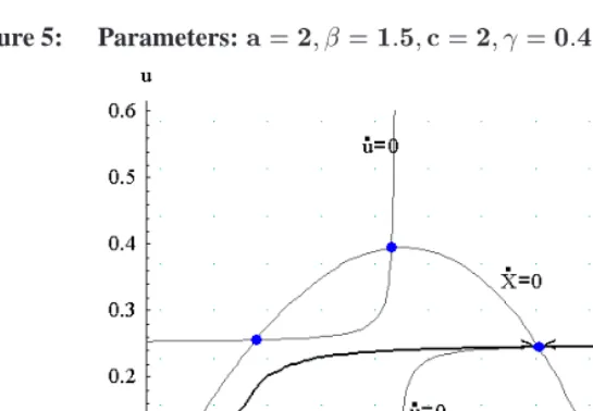
Figure 5: Parameters:a=2; =1:5;c=2;=0:45;r=0:05;=0:02
Note: The middle-size city still dominates. Small and large city (not shown) are suboptimal. The saddle paths to the small city (X=0:23), consisting of a spiral from the vortex (X=0:52) and a path starting at
(X=0:11;u=0) are not shown. If the initial city size is below0:12, it is optimal to have a boundary
solution (u=0) untilX=0:12, and to then follow the saddle path growing to (X=0:834;u=0:245).
6.4 Sensitivity with respect to parametera
The housing market adjustment speed parameter (a) turns out to play a key role in the structure of the optimal housing mobility policy. Whenais rather large, as in our base case, the middle equilibrium withX close to 1 is strong because the uncontrolled com-ponent of the dynamics ( _
X =aX(1 X)) is powerful. One might say that our system displays homeostasis14, and parameterameasures the strength of homeostasis. Just as a strong virus attack can overwhelm a weakened immune system, we can expect that a neighborhood with small (weakened)acan be moved out of its natural equilibrium.
We have already considered several cases for largea = 2, shown in Figs. 1, 3-5. Sometimes there are 4 equilibria, sometimes 2, but there is no policy impact: the middle-size neighborhood is always located near the unperturbed valueX =1and it is always optimal. Small reductions in the value ofado not change this property. Even substantial reduction ofa, from 2 to 0.2 (see Fig. 6) still preserve 4 equilibria: 3 saddles, correspond-ing to low population (X =0:067), normal size (X =0:993) and oversized (X =1:36,
14This term is often used in biological sciences to describe the systems that are able to return to their natural
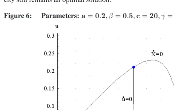
not shown), and one vortex atX =0:61. Besides this complex structure, the middle-size city still remains an optimal solution.
Figure 6: Parameters:a=0:2;=0:5;c=20;=0:45;r=0:05;=0:02
Note: Again, the middle-size city (X=0:993) is optimal, despite the existence of small (X=0:067) and
large (X=1:359, not shown) cities. The vertical dashed line shows the critical set, with the lens at
u=0:025. The horizontal dashed line represents the boundary solution withu=0, which is a part of the
saddle path to the middle-sized city.
Although lower values ofamight be viewed as extreme cases, we should not ignore them for two reasons. First, all of our parameter estimates involve judgments; changing some others can increase the minimum value ofasuch that different behaviors emerge. Second, for whatever reasons, some neighborhoods might have “weakened homeostasis” and correspondingly lowa. For such values ofa, we found several topologically different cases, where an optimal policy destroys the uniqueness of middle-size neighborhood as an optimal solution and sometimes even eliminates it completely.
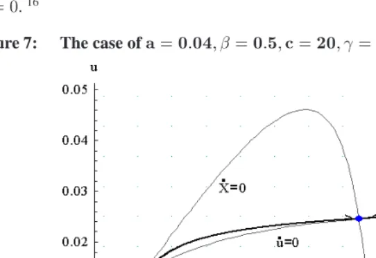
Consider first the case of a = 0:04with high program cost c = 20 (see Fig. 7). Here we still have 4 equilibria, and 3 of them are saddles, representing small, medium size and large city. The main difference is that the unstable steady state becomes a node now, and its location represents a weak Skiba point.15 If we are initially located in the unstable node(X =0:16;u=0:012), we are indifferent between either going to the low equilibrium (which represents complete destruction of the city,(X =0;u=0)for our
parameter set) or to move to middle size city, (X = 0:95;u = 0:024). The oversized city (X = 1:20;u = 0:023)is never optimal because the lens at X = 1:11 passes all trajectories from the right to the left, to converge to the middle-size neighborhood. Only initially small cities, withX(0) <0:16, will eventually converge to the state with
X =0.
16
Figure 7: The case ofa=0:04;=0:5;c=20;=0:45;r=0:05;=0:02
Note: The unstable nodeXs=0:0158is a weak Skiba threshold. Below it, the convergence is to the
disappearing city withX=0, and above it is to the middle-size city withX=0:954. Trajectories starting at
X>X
=1:11(including the saddle path to the middle-size city), pass through the lens at the critical line.
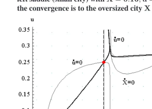
The results are even more dramatic when we reduceato this low level and also use the lower placement cost c = 2. In general, reduction inc leads to higher levels ofu in equilibrium and stronger influence on the system. Fig. 8 shows one such case with
a = 0:05forc = 2. In this case only two saddles are left: small neighborhood, with
X =0:16;u=0:016, and oversized neighborhood, withX=2:26;u=0:27. Since now both solutions play an important role, it is useful to characterize them. In the oversized city the population stock exceeds the normal level by more than a factor of two, and the equilibrium flow of migrants (some of whom assimilate) is very high. At the same time, while the flow of migrants into the small neighborhood remains low, it does not have a capacity to reach more or less normal size. There exists a threshold (strong Skiba point) at
16For slightly different parameter values the small population equilibrium may increase to be on the order of
Figure 8: A Skiba pointXs(between 2 saddles, separated by the critical lineX
) occurs for the parameter valuesa=0:05;=0:5;c=2;=0:45;
r=0:05;=0:02. IfX(0)<Xs=1:21, there is convergence to the
left saddle (small city) withX=0:16;u=0:016, while forX(0)>Xs
the convergence is to the oversized cityX=2:26;u=0:27.
X
S, close to
1:2. If we start at this Skiba threshold, there exist two trajectories, converging to left and right saddles and having identical value of the objective. In other words, atX
S we are indifferent in selecting a path that converges either to heavily undersized or heavily oversized cities.
This case is also interesting mathematically, as it has not previously been described in the dynamic optimization literature. There exists a substantial literature about Skiba points17, but in one-state models a Skiba point typically emerges near a vortex that
sep-arates two saddles. In our case there are just two saddles, separated by a critical line
X =X
=1:11. The lens allows the trajectories to pass from the right to the left. But the direction of the field in the right neighbourhood ofX =X
is such, that two trajecto-ries can coexist only for1:11<X <1:2(see Fig. 9). This means that forX(0)<1:11 there is always a convergence to the low population equilibrium, while forX >1:2there is always a convergence to the high population equilibrium. Hence, there should exist a threshold as the border of these sets, and this can indeed be proven numerically (See Fig. 10 with the details of Skiba point and its neighbourhood).
Figure 9: Detail of Fig. 8, showing the initial parts of the saddle paths around the Skiba pointXs
Note: While foru>0:32the difference between these trajectories is not visible in this illustration, for
topological reasons of course they never intersect. Isoclines, field direction and the lens are also shown.
There exists a third topologically different type of solution with 3 saddles and a vortex. It has been described by Caulkins et al. (2004) but only occurs here if we change simul-taneously several parameters. As in the previous case, the strong Skiba has a threshold
X =X
S(typically X
S
<1, but opposite cases are also discovered), and we converge to the low population equilibrium ifX(0)<X
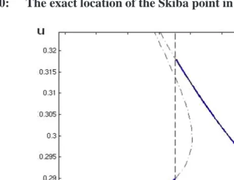
Figure 10: The exact location of the Skiba point in Fig. 8 isXs=1:1975
Note: The initial policyu=0:29leads to the low saddle, while the initial policyu=0:318leads to the
high saddle.
6.5 Bifurcation diagram ina Xspace
It is interesting to examine a bifurcation diagram showing how the topological structure of the solutions varies witha(See Fig. 11). We see that whenais decreased from its basecase value of 2 down to 0.3, there is no topological change, i.e. we continue to have four equilibria. For smaller values ofa, specifically for0:06<a<0:29, we have just two saddles, and the results fora=0:2are as described above. For still smallera(a<0:04), the smallXequilibrium becomes negative (infeasible).
Figure 11: Bifurcation diagram ina Xspace for parameter values:
=0:5;c=2;=0:45;r=0:05;=0:02
Note: Some phase diagrams have been shown already: fora=2see Fig. 1, fora=0:05see Fig. 8. Since
parameter c leads mostly to a change inuand has less influence onX, Fig. 6, drawn fora=0:2andc=20,
topologically corresponds toa=0:2in this diagram.
6.6 Summary of sensitivity with respect to interactions betweenaandc
Reviewing the results above, we observe an interesting interaction between variation (specifically reductions from basecase values) in parameters aandc. Whenais at its (high) basecase value, then variation inc does not alter the basic policy. Even when mobility programs are cheap (cis small), the optimal strategy is always to have the neigh-borhood approach a situation very near its uncontrolled or “natural” state.
However, whenais small, then the strategy depends strongly on the specific value of
c. Whencis at its (high) basecase value, we get a weak Skiba separating the small and medium size equilibria. The mobility program should not be used in a way that alters the basic character of the neighborhood, but if the neighborhood is initially depopulated, the mobility program will be pursued in such a way that the neighborhood never recovers.
7. Conclusions and policy implications
We analyzed a highly stylized model of how poverty deconcentration programs influence population dynamics in the destination neighborhood. The model tracks the stock of middle-class residents and the flow of poor families entering the neighborhood. It consid-ers the effects of both negative externalities that incoming poor families place on current residents (including flight) and positive externalities from middle-class neighborhoods on incoming poor families (through assimilation and directly in the social planner’s objective function). The model is formulated as a dynamic optimization problem faced by a gov-ernmental entity that can control the rate at which the program places poor residents and wishes to do so in a manner that maximizes the discounted weighted sum of net benefits over time.
This model is inspired by policy debates in the US regarding poverty deconcentration through housing mobility initiatives. Typically these discussions, if translated into math-ematics, would have the character of static concave maximization with a unique interior optimum. Recent work has proposed non-monotonic objective functions, emphasized the inadequacy of analyses that focus solely on outcomes for the poor families, and devel-oped policy prescriptions based on static, multi-objective optimization models. However, no prior research known to us has explicitly addressed the dynamic nature of housing mobility policy design.
For base case parameter values we get convergence to a unique equilibrium in which the middle-class population is very close to its uncontrolled or natural level. This result appears to be fairly robust with respect to parameters governing mobility program cost and the extent of middle-class flight induced per poor family placed in the neighborhood. However, if the neighborhood’s underlying population dynamics are not very resilient, in the sense that it can take a long time for population to adjust when it is either above or below the uncontrolled or natural size, then other outcomes may be possible, or indeed optimal. Somewhat similar results can pertain for short-sighted decision makers.
One alternative structure obtained via a “weak” Skiba point might be summarized, “keep the neighborhood in its current state, even if that initial state is de-populated relative to its natural uncontrolled state.” In particular, if the neighborhood is already weakened by under population, then paradoxically creating a new population inflow can prevent the neighborhood from growing because the induced middle-class flight exceeds the as-similation of program participants, in part because the scarcity of current middle-class neighbors undermines that assimilation.
the optimal strategy leads to a “super-populated” neighborhood with population densities above those in the uncontrolled steady state. These outcomes involve high-inflow and high assimilation of poor families into the middle class, but also relatively rapid outflow of middle-class residents in response to both poor families entering and general popula-tion pressure. The resulting transient, high-density neighborhoods might be thought of as akin to those in New York City that traditionally absorbed large numbers of foreign immigrants.
Methodologically one of the most interesting results was finding a critical point that acts as a lens to focus trajectories in state-control space in a manner that lets them pass through a singularity separating two continuous semi-planes. This point seems to be able to separate saddles the way nodes and vortices often do. Because of the continuity of flow through that point, its existence can help reveal what the optimal solution strategy is and how that strategy does and does not depend on various parameters.
Substantively these results have three principal implications. First, inasmuch as the specific quantitative not just qualitative results can be trusted (which is subject to ques-tion given how stylized the model is), it appears that placement rates far in excess of those pursued by the Moving To Opportunity program may be both optimal and unlikely to generate prohibitive levels of middle class flight, at least with basecase parameters. Second, dynamic modeling of population flows related to housing mobility programs can yield interesting, indeed surprising, results and merits further investigation. Third, the likelihood of surprising or structurally different results seems to depend particularly on the dynamic resilience of host neighborhoods, program costs, and the modeling of flight and assimilation. So those topics merit further investigation, particularly from a dynamic perspective. We would highlight in particular the benefits of a refined model with a larger state space to model explicitly the process of upward social mobility over time.
Explicitly specifying functional forms and constraining the state space to dimensions that permit explicit dynamic optimization might inevitably involve a high degree of ab-straction, but the modeling suggests the benefits of realistic quantification of a few at-tributes whose importance exists independent of a dynamic optimization framework. No-tably, how large is the stock of poor families that are eligible for mobility programs rel-ative to the “carrying capacity” of neighborhoods in which they might be placed? In addition, how quickly do each of these stocks grow? Growth for the former pertains to some combination of the rates of upward and downward social mobility combined with the natural reproductive rate for poor families. Growth rates for the latter pertain to how quickly newly placed residents are assimilated, and how flight depends on the rate and accumulation of placed families.
cost-effective, must inevitably be a relative minor complement to core housing programs that help poor families where they are now located. If it is large, then residential mobility programs have the potential to be the primary strategy for meeting housing policy objec-tives. The current model represents a small step toward trying to frame and answer such fundamental questions.
8. Acknowledgements
References
Betts J., Fairlie R.W. (2003). “Does Immigration Induce ’Native Flight’ from Public Schools Into Private Schools?” Journal of Public Economics, Vol. 87, No. 5-6: 987-1012.
Caulkins J., Feichtinger G., Johnson M., Tragler G., Yegorov Y. (2004). “Skiba Thresh-olds in a Model of Controlled Migration.” Journal of Economic Behaviour and Or-ganization, accepted for publication.
Caulkins J., Pacula R., Paddock S., Chiesa J. (2002). School-Based Drug Prevention: What Kind of Drug Use Does it Prevent? Santa Monica, CA: RAND (MR-1459-RWJ).
Chiang A. (1992). Elements of dynamic optimization. New York: McGraw-Hill.
Clotfelter C.T. (2001). “Are Whites Still Fleeing? Racial Patterns and Enrollment Shifts in Urban Public Schools, 1987-1996.” Journal of Policy Analysis and Management, Vol. 20, No. 2: 199-221.
Cohen M. (1998). “The Monetary Value of Saving a High-Risk Youth.” Journal of Quan-titative Criminology, Vol. 14, No. 1: 5-33.
Deissenberg C., Feichtinger G., Semmler W., Wirl F. (2004). Multiple equilibria, history dependence, and global dynamics in intertemporal optimization models. In: Barnett W.A., Deissenberg C., Feichtinger G., editors. Economic Complexity: Non-linear Dynamics, Multi-agents Economies, and Learning. Amsterdam: Elsevier.
DeLuca S., Rosenbaum J.E. (2003). “If Low-Income Blacks Are Given a Chance to Live in White Neighborhoods, Will They Stay? Examining Mobility Patterns in a Quasi-Experimental Program with Administrative Data.” Housing Policy Debate, Vol. 14, No. 3: 305-345.
DeMarco D.L., Galster G.C. (1993). “Prointegrative Policy: Theory and Practice.” Jour-nal of Urban Affairs, Vol. 15, No. 2: 141-160.
Fairlie R.W. (2002). “Private Schools and ’Latino Flight’ from Black Schoolchildren.” Demography, Vol. 39, No. 4: 655-674.
Feichtinger G., Hartl R.F. (1986). Optimale Kontrolle ¨okonomischer Prozesse – Anwen-dungen des Maximumprinzips in den Wirtschaftswissenschaften. Berlin: Walter de Gruyter.
Freeman L., Rohe W. (2000). “Subsidized Housing and Neighborhood Racial Transition: An Empirical Investigation.” Housing Policy Debate, Vol. 11, No. 1: 67-89.
Galster G. (1988). “Residential Segregation in America: A Contrary Review.” Population Research and Policy Review, Vol. 7: 93 - 212.
Galster G. (1998). “A Stock/Flow Model of Defining Racially Integrated Neighborhoods.” Journal of Urban Affairs, Vol. 20, No. 1: 43-51.
Galster G. (2002). “An Economic Efficiency Analysis of Deconcentrating Poverty Popu-lations.” Journal of Housing Economics, Vol. 11: 303-329.
Galster G.C., Tatian P., Smith R. (1999). “The Impact of Neighbors Who Use Section 8 Certificates on Property Values.” Housing Policy Debate, Vol. 10, No. 4: 879-917.
Gould Ellen I. (2000). Sharing America’s Neighborhoods: The Prospects for Stable Racial Integration. Cambridge, Mass.: Harvard University Press.
Jargowsky P.A. (1996). “Take the Money and Run: Economic Segregation in U.S. Metropoli-tan Areas.” American Sociological Review, Vol. 61: 984-998.
Johnson M.P., Hurter A.P. (2000). “Decision Support for a Housing Relocation Program Using a Multi-Objective Optimization Model.” Management Science, Vol. 46, No. 12: 1569-1584.
Johnson M.P., Ladd H.F., Ludwig J. (2001). “The Benefits and Costs of Residential-Mobility Programs for the Poor.” Housing Studies, Vol. 17, No. 1: 125-138.
Massey D.S., Gross A.B., Eggers M.L. (1991). “Segregation, the Concentration of Poverty, and the Life Chances of Individuals.” Social Science Research, Vol. 20, No. 4: 397-420.
Mayer S.E., Jencks C. (1989). “Growing Up In Poor Neighborhoods: How Much Does It Matter?” Science, Vol. 243, No. 4897: 1441-1445.
Murphy P. (1995). “Black Flight: Years of Liberal Government Drives Away D.C.’s Mid-dle Class.” Policy Review, Vol. 72: 28-35.
Office of National Drug Control Policy (ONDCP). (2002). The National Drug Strategy. Washington, DC: The WhiteHouse.
Popkin S.J., Rosenbaum J.E., Meaden P.M. (1993). “Labor Market Experiences of Low-Income Black Women in Middle-Class Suburbs: Evidence from a Survey of Gautre-aux Program Participants.” Journal of Policy Analysis and Management, Vol. 12, No. 3: 556-573.
Rosenbaum J.E. (1995). “Changing the Geography of Opportunity by Expanding Resi-dential Choice: Lessons from the Gautreaux Program.” Housing Policy Debate, Vol. 6, No. 1: 231-269.
Santiago A.M., Galster G.C., Tatian P. (2001). “Assessing the Property Value Impacts of the Dispersed Housing Subsidy Program in Denver.” Journal of Policy Analysis and Management, Vol. 20, No. 1: 65-88.
Schelling T. (1971). “Dynamic model of segregation.”, Journal of Mathematical Sociol-ogy, Vol. 1: 143-186.
Schelling T. (1973). “Hockey helmets, concealed weapons, and daylight saving: a study of binary choices with externalities.” Journal of Conflict Resolution, Vol. 17, No. 3: 381-428.
Shroder M. (2001). “Moving to Opportunity: An Experiment in Social and Geographic Mobility.” Cityscape: A Journal of Policy Development and Research, Vol. 5, No. 2: 57-67.
U.S. Census Bureau. (2004a). http://www.census.gov/const/stageann.prf.
U.S. Census Bureau. (2004b).
http://www.census.gov/ hhes/www/housing/ahs/ahs01/Tab1a.html.
U.S. Department of Housing and Urban Development. (1999). Moving to Opportunity for Fair Housing Demonstration Program: Current Status and Initial Findings. Wash-ington, D.C.: Office of Policy Development and Research.
World Wide Web: http://www.huduser.org/publications/pdf/mto.pdf.
U.S. Department of Housing and Urban Development. (2003). Moving To Opportunity for Fair Housing Demonstration Program: Interim Impacts Evaluation. Washing-ton, D.C.: Office of Policy Development and Research.
Wilson W.J. (1987). The Truly Disadvantaged. Chicago, IL: University of Chicago Press.