R E S E A R C H A R T I C L E
Open Access
Estimation of seismic velocity changes at
different depths associated with the 2014
Northern Nagano Prefecture earthquake,
Japan (
M
W
6.2) by joint interferometric
analysis of NIED Hi-net and KiK-net records
Kaoru Sawazaki
*, Tatsuhiko Saito, Tomotake Ueno and Katsuhiko Shiomi
Abstract
To estimate the seismic velocity changes at different depths associated with a large earthquake, we apply passive image interferometry to two types of seismograms: KiK-net vertical pairs of earthquake records and Hi-net continuous borehole data. We compute the surface/borehole deconvolution waveform (DCW) of seismograms recorded by a KiK-net station and the autocorrelation function (ACF) of ambient noise recorded by a collocated Hi-net station, 26 km from the epicenter of the 2014 Northern Nagano Prefecture earthquake, Japan (MW6.2). Because the deeper KiK-net sensor and the Hi-net sensor are collocated at 150 m depth, and another KiK-net sensor is located at the surface directly above the borehole sensors, we can measure shallow (<150 m depth) and deep (>150 m depth) velocity changes separately. The sensitivity of the ACF to the velocity changes in the deeper zone is evaluated by a numerical wave propagation simulation. We detect relative velocity changes of−3.1 and−1.4% in the shallow and deep zones, respectively, within 1 week of the mainshock. The relative velocity changes recover to
−1.9 and−1.1%, respectively, during the period between 1 week and 4 months after the mainshock. The observed relative velocity reductions can be attributed to dynamic strain changes due to the strong ground motion, rather than static strain changes due to coseismic deformation by the mainshock. The speed of velocity recovery may be faster in the shallow zone than in the deep zone because the recovery speed is controlled by initial damage in the medium. This recovery feature is analogous to the behavior of slow dynamics observed in rock experiments.
Keywords:Time-lapse monitoring, Velocity change and recovery, Passive image interferometry, Wave propagation simulation, Dynamic and static strain changes, Slow dynamics
Introduction
Even though seismic velocity changes associated with large earthquakes have been widely studied for decades (e.g., Poupinet et al. 1984), the cause of the observed velocity changes is still debated. Seismic motion is sig-nificantly amplified in low-velocity sediments and some-times induces severe damage to the shallow subsurface (e.g., Rubinstein and Beroza 2005; Sawazaki et al. 2009). On the other hand, static crustal deformation as-sociated with a large earthquake also induces damage to
the subsurface medium, in particular near the earth-quake fault (e.g., Brenguier et al. 2008). Both dynamic (strong ground motion) and static (crustal deformation) strain changes are the possible causes of observed seis-mic velocity changes. However, it is difficult to evaluate the contribution of each factor to seismic velocity changes because the spatial resolutions of the velocity changes associated with these phenomena are poorly understood.
To detect shallow velocity changes separately from changes at greater depths, previous studies used pairs of seismograms from vertically offset instruments, e.g., paired sensors in a single vertical borehole (e.g., * Correspondence:[email protected]
National Research Institute for Earth Science and Disaster Resilience, Tsukuba, Japan
Sawazaki et al. 2009; Nakata and Snieder 2012; Takagi et al. 2012). According to these studies, velocity reduc-tion is concentrated in the topmost layers (generally shallower than several hundred meters) because the layers are severely damaged by strong ground motion. On the other hand, some studies have detected velocity changes associated with earthquake swarms (e.g., Maeda et al. 2010; Ueno et al. 2012), postseismic deformation (e.g., Brenguier et al. 2008), and slow slip (e.g., Rivet et al. 2011), which are not accompanied by strong ground motion. This suggests that both dynamic and static strain changes are likely to cause velocity changes and that their relative contributions may change with depth.
The sensitivity of the seismic wavefield can also be used to estimate velocity changes in shallow and deep zones separately. Hobiger et al. (2012) analyzed the dif-ferent frequency ranges of the cross-correlation func-tions of ambient noise records and reported that velocity reduction due to a large earthquake is larger at higher frequencies. Because surface waves are more sensitive to shallow structure at high frequencies, this result suggests that velocity reduction is more significant at shallower depths. Recently, the sensitivity kernel of the seismic wavefield, reconstructed by analytical (e.g., Pacheco and Snieder 2005, 2006) and numerical (e.g., Obermann et al. 2013a; Kanu and Snieder 2015) approaches, has been used in an inversion scheme that can resolve spatial variations in velocity changes (e.g., Obermann et al. 2013b). A more direct approach that uses the sen-sitivity of the phase delay curves to partial velocity changes has been developed to investigate spatial varia-tions (e.g., Yang et al. 2014; Sawazaki et al. 2015). How-ever, because the accuracy of the sensitivity kernel strongly depends on the short-wavelength velocity struc-ture, which is not sufficiently determined in most areas, the utility of the sensitivity kernel is still limited, espe-cially with respect to depth resolution.
To further investigate the seismic velocity changes as-sociated with large earthquakes at different depths, verti-cal pairs of seismograms and sensitivity of the seismic wavefield should be used in combination. In this study, we apply the passive image interferometry technique (e.g., Sens-Schönfelder and Wegler 2006) to two differ-ent types of collocated seismometers. The first is a verti-cal pair of strong motion accelerometers from KiK-net, installed at the surface and the bottom of a borehole (150 m deep). The second is a Hi-net high-sensitivity seismometer collocated with the KiK-net borehole bot-tom accelerometer (Fig. 1b). Both seismograph networks are operated by the National Research Institute for Earth Science and Disaster Resilience (NIED) of Japan (Okada et al. 2004). The surface/borehole deconvolution wave-form (DCW) of the KiK-net seismograms is suitable to
reconstruct the transfer function from 150 m depth to the surface (Snieder andŞafak 2006). Hi-net continuous records are suitable for reconstructing the autocorrel-ation function (ACF) of the ambient noise (e.g., Ueno et al. 2015), which approximately represents the zero-offset Green’s function (Claerbout 1968). The retrieved DCW is sensitive to changes in the medium above 150 m depth, while the ACF is sensitive to changes in the medium both above and below 150 m. To evaluate the sensitivity of the ACF to the partial velocity changes above and below the 150 m depth cutoff, we perform a numerical wave propagation simulation based on a real-istic velocity model. We then independently estimate the velocity changes above and below the 150 m depth cut-off associated with theMW6.2 Northern Nagano Prefec-ture earthquake, Japan (hereafter referenced as the “N. Nagano earthquake”), which occurred on 22 November 2014. From the velocity changes and recoveries observed at different depths, and susceptibility values previously estimated in rock experiments, we discuss the contribu-tions of dynamic and static strain changes to the damage at the subsurface.
Methods/Experimental
We use data from Hi-net station N.MKGH and collo-cated KiK-net station NIGH17, 26 km from the epicen-ter of the N. Nagano earthquake (Fig. 1a). The Hi-net and KiK-net borehole sensors are installed at 150 m depth, while another KiK-net sensor is installed at the ground surface (Fig. 1b). A continuous record is avail-able for Hi-net, while only event-triggered records are available for KiK-net. Both Hi-net and KiK-net systems sample ground oscillations at a frequency of 100 Hz. The frequency response of the Hi-net seismometer is flat from 1 to 30 Hz, while that of the KiK-net seismometer is flat from DC to about 20 Hz. Details of the Hi-net and KiK-net recording systems are summarized by Okada et al. (2004).
There are several Hi-net (KiK-net) stations around the source region of the N. Nagano earthquake.
How-ever, only E−W component data from stations
N.MKGH and NIGH17 are available for combined analysis of KiK-net and Hi-net records, for reasons explained in the next section.
Processing of KiK-net records
Nagano earthquake). To avoid apparent velocity changes due to variations in incidence angle, we select earth-quake records that satisfy the condition that the S-wave incidence angle to the borehole bottom sensor is <22°. From each seismogram in each period, we extract a se-quence of 10.24 s non-overlapping time windows that begins at the S-wave onset time and ends in the S-wave coda. We limit the value of the maximum dynamic strain (MDS) measured for each time window to smaller than 5 × 10⁻⁶and larger than 5 × 10⁻⁹for both the bore-hole bottom and the surface KiK-net sensors. Here, the maximum limit corresponds to the threshold of emer-gence of nonlinear site response effects (e.g., Beresnev and Wen 1996), and the minimum limit corresponds to about 10× the average amplitude of the ambient back-ground noise. The MDS is computed by dividing the peak ground velocity (PGV) by the S-wave velocity in the medium, whereVS30and VS at 150 m depth denote
the S-wave velocities at the surface and the borehole bottom, respectively. For each windowed trace, we apply a 1–10 Hz 4-pole Butterworth bandpass filter to the sur-face/borehole deconvolution waveform (DCW). Then, we average all DCWs obtained in each period. The num-bers of DCWs used for averaging in each period are 117, 55, and 30, for the reference period, period 1, and period 2, respectively.
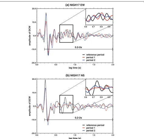
Figure 2 shows the averaged DCWs for the E−W (Fig. 2a) and N−S (Fig. 2b) components of motion in each of the three time periods. The peaks of the DCWs, which appear around a lag time of 0.23 s, represent one-way S-wave travel times from the borehole bottom to the ground surface. The S-wave travel time computed from well logging data is 0.25 s. After the arrival of the peak, we see that reverberated waves, excited in the layers between the surface and the borehole bottom KiK-net sensor, appear in the DCWs.
(a)
137.6˚ 137.8˚ 138.0˚ 138.2˚ 138.4˚
36.6˚ 36.8˚ 37.0˚
0 10 20
km
N.MKGH&NIGH17
Futagojima
-1×10⁻⁵
0 1×10⁻⁵
0
5
10
15
20
Depth (km)
εS
150m
KiK-net (surface)
KiK-net (borehole)
Hi-net N.MKGH&NIGH17
(b)
geology:
madlayer, tuff breccia,
sandy gravel, andesite
Fig. 1aHypocenter of the 2014 Northern Nagano Prefecture earthquake (focal mechanism). The location of collocated stations N.MKGH (Hi-net) and NIGH17 (KiK-net) is indicated by awhite triangle. Blue triangleindicates the location of Futagojima station, which monitors the streamflow of the Seki-river.
The waveforms of the E−W component are similar at different time periods; clear phase delays with re-spect to the reference period are recognized in pe-riods 1 and 2. On the other hand, the waveforms of the N−S component are relatively dissimilar at differ-ent time periods. The shapes of the waveforms in pe-riods 1 and 2 are considerably different from the shape of the reference period waveform. Because the recording system response and noise amplitude are almost the same for both components throughout the analyzed period, we consider that the N. Nagano
earthquake excited anisotropic damage to the
subsurface medium (e.g., Nakata and Snieder 2012), and consequently the DCW of the N−S component data changed more radically than that of the E−W component. Because the stretching technique (Wegler and Sens-Schönfelder 2007) is not applicable to a dis-similar waveform pair, we apply the stretching tech-nique only to the E−W component to estimate the
relative velocity change after the N. Nagano
earthquake.
The lag time used for stretching begins at 0.2 s and ends at 2.0 s (see Fig. 2), within which the DCW is sensi-tive mostly to the medium between the two sensors -20.0
-10.0 0.0 10.0 20.0
amplitude of DCW
0.0 0.5 1.0 1.5 2.0
lag time (s)
(a) NIGH17 EW
0.2-2s
reference period period 1 period 2
0.6 0.7 0.8 0.9
-20.0 -10.0 0.0 10.0 20.0
amplitude of DCW
0.0 0.5 1.0 1.5 2.0
lag time (s)
(b) NIGH17 NS
0.2-2s
reference period period 1 period 2
0.6 0.7 0.8 0.9
(<150 m depth). The error of the estimated relative vel-ocity change is computed using the formula proposed by Weaver et al. (2011):
err¼
ffiffiffiffiffiffiffiffiffiffiffi
1−C2
p
2C
ffiffiffiffiffiffiffiffiffiffiffiffiffiffiffiffiffiffiffiffi
6pffiffiffiffiffiffiffiffiπ=2T
ω2
Cðt32−t31Þ s
; ð1Þ
whereC,T,ωC,t1, andt2are the maximum coherence value of the correlation coefficient, the inverse of the fre-quency bandwidth, the central angular frefre-quency of the passband, and the start and end of the lag times used for the stretching technique, respectively.
Processing of Hi-net records
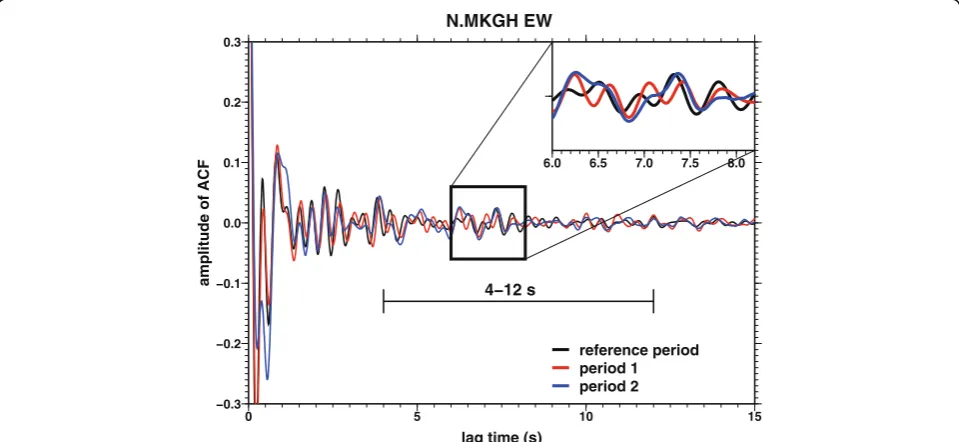
We first apply a 1–3 Hz 4-pole Butterworth bandpass filter to the E−W component of the Hi-net data, then apply one-bit normalization to suppress signals from earthquakes and other nonstationary phenomena. We then compute the autocorrelation function (ACF) using 1-hour time segments and average the ACFs obtained in each period. By applying the stretching technique to the ACFs obtained in the reference period to match the ACFs from periods 1 and 2, we compute the apparent relative velocity change after the N. Nagano earthquake. The lag time used for stretching begins at 4 s and ends at 12 s (see Fig. 3). Again, the error of the apparent rela-tive velocity change is computed using Eq. (1).
Figure 3 shows the averaged ACFs obtained for each period. The inset figure shows a small phase delay in pe-riods 1 and 2 with respect to the reference period, which can be attributed to a subsurface velocity reduction. Be-cause the ACF can be regarded as the zero-offset Green’s
function (Claerbout 1968), the ACF at 4–12 s lag is sen-sitive to the medium change within about 20 km of the Hi-net sensor if we assume VS= 3.4 km/s and single backscattering. Therefore, the velocity change near the fault zone (mostly >20 km from N.MKGH) is hardly sensed by the ACF for the range of lags considered. At this stage, we do not know how much of the change in the ACF can be attributed to the velocity changes below the installation depth (150 m) of the Hi-net sensor. It is necessary to evaluate the sensitivity of the ACF to esti-mate the velocity change below the installation depth; the procedure for this will be described later.
Correcting for seasonal velocity variations
Seismic velocity may exhibit seasonal variations (e.g., Meier et al. 2010) that are not caused by nonstationary phenomena like earthquakes. Figure 4a shows the varia-tions in apparent relative velocity change from Novem-ber 2009 to July 2015, where each point is a 1-week average of ACFs at station N.MKGH. In addition to the apparent velocity reductions after the Tohoku earth-quake (MW 9.0) on 11 March 2011, and the N. Nagano earthquake on 22 November 2014 (red arrows), the rela-tive velocity changes show clear seasonal variations. Note that the RMS noise amplitude recorded at station N.MKGH (gray dots in Fig. 4) also shows a seasonal change, where the period of large RMS noise amplitude (April to May) corresponds to that of rapid velocity re-duction and a low correlation coefficient. Because N.MKGH is located in a heavy snowfall zone, meltwater in spring induces strong streamflow and consequently may increase the amplitude of the ambient noise (e.g.,
−0.3 −0.2 −0.1 0.0 0.1 0.2 0.3
amplitude of ACF
5 1 0
1 5
0
lag time (s)
W E H G K M . N
reference period period 1 period 2
4−12 s
6.0 6.5 7.0 7.5 8.0
Burtin et al. 2008). As shown in Fig. 5, a clear correl-ation is observed between the RMS noise amplitude (gray) and the streamflow of the Seki River at Futago-jima monitoring station (blue, operated by the Ministry of Land, Infrastructure, Transport and Tourism, Japan; see Fig. 1), especially during the season of heavy stream-flow (Fig. 5b). Therefore, the primary cause of the sea-sonal velocity variations is the change of the noise source distribution due to increased streamflow, and fol-lowing changes in the groundwater system.
To separate earthquake-origin velocity changes from observed seasonal velocity changes, we fit a sine curve to the estimated seasonal velocity variations (e.g., Hobiger et al. 2012), excluding three time pe-riods: within a year of the Tohoku earthquake (11 March 2011 to 11 March 2012), a period of recording system errors (10 November 2012 to 16 May 2013), and the post-N. Nagano earthquake period (22 No-vember 2014 onward). We then subtract the sine curve from the raw data and use the subtracted data as the apparent relative velocity change (Fig. 4b). In addition to the velocity reductions due to the two large earthquakes, the corrected apparent relative vel-ocity change also shows a large velvel-ocity reduction in April to May 2015. Although similar velocity reduc-tions appear in this season every year, the 2015 case is much more significant than in other years and can-not be removed completely by subtraction of the fit-ted sine curve. One reason for this velocity reduction
could be that the strong ground shaking and
generation of cracks by the 2014 N. Nagano earth-quake made the subsurface structure more susceptible to external changes, though this hypothesis is not supported by other observations. On the other hand, we do not correct the seasonal variations in velocity change obtained from the KiK-net DCWs because the data from KiK-net records are so sparse that seasonal variations cannot be confirmed.
Sensitivity of ACF to partial velocity changes
The relative velocity changes detected by the KiK-net DCWs and Hi-net ACFs (ΔV/VKiK and ΔV/VHi, re-spectively) are sensitive to velocity changes in differ-ent zones. The former is sensitive only to the medium at <150 m depth (the “shallow zone”), while the latter is sensitive to the medium both above and below 150 m depth (the latter is herein called the “deep zone”). To extract the velocity change in the deep zone from the values of ΔV/VKiK and ΔV/VHi, we evaluate the sensitivity of the ACF to partial vel-ocity changes in the deep zone through a two-dimensional wave propagation simulation using the fi-nite difference method (FDM). We do not perform a three-dimensional simulation because of the limita-tions of computation time. The most significant dif-ference between 2D and 3D simulations that affects the sensitivity should be the S/P energy partition, which has values of 3.0 and 10.4 in an equilibrium state for the 2D and 3D cases, respectively (e.g., Sán-chez-Sesma and Campillo 2006). Therefore, we apply 100
101
102
103
104
105
rms amplitude (nm/s)
−0.03 −0.02 −0.01 0.00 0.01 0.02 0.03
V/V
Hi
2010 2011 2012 2013 2014 2015
Year
(a) before annual correction
2014/11/22 N.Nagano 2011/3/11
Tohoku
100
101
102
103
104
105
rms amplitude (nm/s)
−0.03 −0.02 −0.01 0.00 0.01 0.02 0.03
V/V
Hi
2010 2011 2012 2013 2014 2015
Year
(b) after annual correction
2014/11/22 N.Nagano 2011/3/11
Tohoku
0.0 0.5 1.0
correlation coefficient
the same velocity perturbations for both VP and VS when evaluating the sensitivity, in order not to distin-guish changes of VP and VS. The geometrical spread-ing factor is also different for the 2D and 3D cases; however, because we do not use waveform amplitude to evaluate sensitivity, these differences will not affect our outcome significantly.
We assume that the ACF of the Hi-net ambient noise records approximately represents the Green’s function (Claerbout 1968), where both the source and the receiver are located at the position of the Hi-net sensor (150 m depth). We note that the pas-sive image interferometry technique is available for time-lapse monitoring if the noise source distribu-tion is temporally stable, even though the spatial dis-tribution of the noise source may not be uniform
and the Green’s function may not be correctly
re-trieved (Hadziioannou et al. 2009). Since possible bias due to seasonal variations in the noise source distribution would be corrected by the procedure ex-plained in the previous section, using the numerical
Green’s function to approximate the observed ACF
is appropriate for our purposes. Therefore, we set a horizontal single point force at 150 m depth and re-produce the horizontal waveform at the same
loca-tion (Fig. 6a), which is regarded as the
corresponding ACF. We use a Küpper wavelet with a central frequency of 2 Hz as the source-time func-tion considering the 1 to 3 Hz bandpass filter ap-plied to the observed Hi-net record.
For the medium below 2.5 km, the background 1D velocity structure is estimated from the results of
100 101 102 103 104
rms amplitude (nm/s)
10−1 100 101 102 103
streamflow (m
3/s)
2011/01 2011/07 2012/01 2012/07 2013/01 2013/07
year/month
(a) 2011/01/01−2013/12/31
rms amplitude streamflow
100 101 102 103 104
rms amplitude (nm/s)
10−1 100 101 102 103
streamflow (m
3/s)
2012/04/01 2012/04/16 2012/05/01 2012/05/16 2012/05/31
year/month/day
(b) 2012/04/01−2012/05/31
rms amplitude streamflow
velocity tomography by Matsubara and Obara (2011). For the shallower medium, we use well log data from station NIGH17 with a deep subsurface structure model provided by J-SHIS (Fujiwara et al. 2009). We then generate five 2D velocity structures by superim-posing five seeds of exponential-type random velocity fluctuations (e.g., Sato et al. 2012) on the 1D velocity structure. For random fluctuation parameters, we set ε= 0.06 (fractional velocity fluctuation), ax= 600 m (horizontal correlation length), and az= 200 m (verti-cal correlation length), based on field measurements by Holliger and Levander (1992). The quality factor Q
is adopted from the 1D reference model provided by
J-SHIS. The mass density of the medium is ρ¼310
V0P:25 following the empirical formula of Gardner
et al. (1974), where the measurement units of ρ and
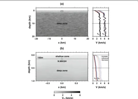
VP are kg/m3 and m/s, respectively. Figure 6 shows an example of the velocity profile used in the numer-ical simulations. The model covers a horizontal region of 100 km to a depth of 50 km (not shown fully in
Fig. 6) and is discretized in grid intervals of 25 m. Free surface and absorbing boundary conditions are employed for the top surface (z= 0 km) and the other three boundaries of the computation area, respect-ively; these conditions avoid numerical divergence and numerical dispersion. The temporal sampling interval is 0.0015 s.
To evaluate the sensitivity of the ACF to partial vel-ocity changes, the numerical waveforms are computed for the reference and perturbed velocity structures. The perturbed structures are reconstructed by apply-ing a 3% velocity reduction to the reference medium at depths of 0–150 m (above the location of the sen-sor) and 150 m to 50 km (below the location of the sensor) individually. We call these zones the “shallow” and “deep” zones, respectively, as shown in Fig. 6b. Applying the stretching technique to the reference and perturbed waveforms using lag times of 4–12 s, we compute the travel time shifts τshallow and τdeep due to the 3% velocity reductions in the shallow and
0
10
20
depth (km)
−20 −10 0 10 20
x (km)
(a)
deep zone
0 2 4 6 8
V (km/s) VP
VS
0.0
0.5
1.0
depth (km)
−0.5 0.0 0.5
x (km)
(b)
N.MKGH 150m shallow zone
deep zone
0 2 4 6 8
V (km/s) VP
VS
increase reference decrease
0 2 4 6
VS (km/s)
deep zones, respectively. The sensitivity to the deep zone α is given by
α¼ τdeep
τshallowþτdeep: ð
2Þ
We consider that the observed relative velocity change ΔV/VHi is approximately given by the weighted sum of the partial relative velocity changes,
ΔV
V Hi≈ð1−αÞ
ΔV
V shallowþα
ΔV
V deep; ð3Þ
where ΔV/Vdeep and ΔV/Vshallow represent the true relative velocity changes in the deep and shallow zones, respectively. Equation (3) is a good approximation when the relative velocity change is much smaller than unity (e.g., Snieder 2006; see also Appendix A). Because ΔV/
VHi and ΔV/Vshallow(=ΔV/VKiK) are obtained directly from the observations, we can estimate the value ofΔV/
Vdeeponce we obtain the sensitivityα.
Results and Discussion
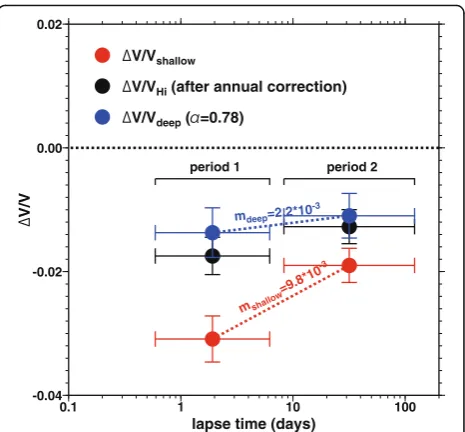
The evaluated sensitivity α is 0.78 under the reference velocity structure. This value indicates that almost 80% of the ACF energy senses changes in the medium below the Hi-net sensor installation depth of 150 m. Using this αvalue and Eq. (3), we plotΔV/Vdeepin Fig. 7 (blue cir-cles), as well as the relative velocity change detected from the DCW of the KiK-net records (ΔV/Vshallow, red circles) and from the ACF of the Hi-net records (ΔV/
VHi, black circles). In period 1, the estimated relative
vel-ocity changes are −3.1 and −1.4% in the shallow and
deep zones, respectively. In period 2, the relative velocity changes recover to −1.9 and −1.1% in the shallow and deep zones, respectively.
The value of α= 0.78 is evaluated using the reference velocity structure, which may include biases from the true velocity structure. Therefore, it is important to evaluate how much theα value could be perturbed due to uncertainty in the reference velocity structure. We verify the range of sensitivities α using different refer-ence velocity structures reproduced by decreasing and increasing the reference velocities above 2.5 km depth by up to 20%, as shown by the red and blue 1D velocity profiles in Fig. 6, respectively. The evaluatedαvalues are 0.75 and 0.82 for decreased and increased velocities, re-spectively. As the velocity of the shallow zone decreases, more of the energy of the ACF is trapped by the shallow layers; consequently, the ACF becomes more sensitive to the velocity change in the shallow zone and the αvalue decreases.
Using Eq. (3), we draw the αdependence of ΔV/Vdeep in Fig. 8, where ΔV/Vshallowand ΔV/VHiare fixed at the observed values. As derived from Eq. (3), the value of
ΔV/Vdeepis equal toΔV/VHiwhenα= 1. In this case, the ACF is sensitive only to the velocity change in the deep zone. As α becomes smaller, ΔV/Vdeep and its standard deviation increase, and both diverge to infinity whenα= 0. In this case, the ACF has no sensitivity to change in the deep zone, which means we cannot obtain any infor-mation about the velocity change below 150 m. From Fig. 8, we confirm that the value of ΔV/Vdeepdoes not change drastically within the evaluated range ofα(from 0.75 to 0.82, as indicated by the white background).
Contribution of dynamic and static strain changes to velocity change
To investigate the cause of the velocity changes observed at different depths, we now examine the contributions of dynamic and static strain changes due to the N. Nagano earthquake as the candidate of the cause.
For the N. Nagano earthquake, the maximum dynamic strains (MDS) recorded at station NIGH17 are εD
surface
¼5:310−4 and εD
borehole ¼1:410−4 at the surface
and the borehole bottom, respectively. These values can constrain the range of the MDS in the shallow zone. In the deep zone, on the other hand, we indirectly evaluate the MDS through the results of the numerical wave propagation simulation. Using the reference velocity structure shown in Fig. 6 and setting a 0.5 Hz Küpper wavelet as a source waveform (since 0.5 Hz is the
-0.04 -0.02 0.00 0.02
V/V
0.1 1 10 100
lapse time (days) V/Vshallow
V/VHi (after annual correction)
V/Vdeep ( =0.78)
mdeep=2.2*10 -3
mshallow
=9.8*10
-3
period 1 period 2
Fig. 7Relative velocity changes estimated for the shallow (red circles) and deep (blue circles) zones, whereα= 0.78 is used for the latter. Relative velocity changes detected from the Hi-net ACF are shown byblack circles. Theabscissaindicates the lapse time after the N. Nagano earthquake, plotted with a logarithmic scale. Them
dominant frequency of the observed velocity seismo-gram) to the position that corresponds to the hypocenter of the N. Nagano earthquake (x=–25.9 km, z= 4.6 km), we synthesize the numerical waveforms of the horizontal
component at positions x= 0 km, z= 150 m and x=
0 km, z= 5 km. The 5 km depth is considered because below which the ACF has almost no sensitivity, accord-ing to our numerical tests. We obtain a ratio of com-puted MDS values at 5 km depth/MDS at 150 m depth of εD
5km=εD150m¼0:091. We then calculate an MDS value
at 5 km depth of εD
5km¼0:091εboreholeD ¼1:310−5
for the N. Nagano earthquake. We note that this evalu-ation may include a large bias due to the difference
be-tween geometrical spreading factors for the 2D
(numerically simulated) and 3D (observed) media. Using these values, we evaluate the possible ranges of MDS values in the shallow and deep zones as 1:410−4≤
εD
shallow≤5:310−4 and 1:310−5≤εDdeep≤1:410−4 ,
respectively.
Next, we compute the coseismic static strain change beneath station N.MKGH using the code of Okada (1992) and a rectangular plane fault model (20 km long and 14 km width) for the N. Nagano earthquake (quadrangle in Fig. 1). Here, the focal mechanism is adopted from the CMT solution (strike = 22°, dip = 51°, rake = 62°) of F-net (the Full Range Seismograph Network of Japan, operated by NIED). A slip of 0.4 m is uniformly distributed on the rectangular fault. The corresponding seismic moment is 3.4 × 10¹⁸ (Nm) =MW 6.3, which is close to the reported value. Our computed ranges of the static volumetric strain
change (SVSC) are −3:7310−7≤εS
shallow≤−3:6810−7
and −3:710−7≤εS
deep≤−1:510−7 in the shallow (0–
150 m depth) and deep (150 m–5 km) zones, respect-ively, where the minus sign indicates contraction. The distributions of SVSC are mapped in Fig. 1a by col-ored grids.
Figure 9 compares the observed relative velocity change in period 1 and the evaluated ranges of MDS (solid circles) and SVSC (open symbols) in the shallow and deep zones. Although the evaluated SVSC has nega-tive values, we show their absolute values in Fig. 9 for the sake of discussion. The values of MDS are larger than SVSC in both the shallow and deep zones by ~102– 103. In the same figure, we also show the values of sus-ceptibility (relative velocity change with respect to the applied strain change, given by ΔV/V/ε) with gray curves. If the observed velocity reduction is caused mainly by the dynamic strain change, then the value of susceptibility should be approximately −1000 to −100 for both zones. On the other hand, if the observed vel-ocity reduction is caused mostly by the static strain change, then the susceptibility should be around−105.
We now compare these calculated values with suscep-tibilities measured in rock experiments. According to Prioul et al. (2004), the values of the third-order elastic constants (TOE), which give the variability of material with respect to the applied static stress change (e.g.,
−0.03 −0.02 −0.01 0.00 0.01
V/V
deep
0.0 0.2 0.4 0.6 0.8 1.0
period 1 period 2
reference model ( =0.78)
Fig. 8αvalue-dependence of the relative velocity change in the deep zone. Theblack and gray curvesrepresent values evaluated in periods 1 and 2, respectively.Broken curvesrepresent the ranges of the corresponding error bars. The area with awhite background
represents a range ofαvalues evaluated using the decreased (α= 0.75) and increased (α= 0.82) reference velocity structures
-0.04 -0.03 -0.02 -0.01 0.00
V/V
10-7 10-6 10-5 10-4 10-3
strain change MDS
SVSC
possible range from rock experiment
deep zone
shallow zone
sus=-100000 sus=-10000 sus=-1000 sus=-10
0
Fig. 9Relationship between the observed relative velocity change
ΔV/Vin period 1, and dynamic (solid circles) and static (open symbols) strain changes in the shallow and deep zones at station N.MKGH.
Murnaghan 1967), are c111=−11300, c123= 5800, and
c111=−3100 GPa, c123= 40 GPa under hydrostatic stresses of 5–30 and 30–100 MPa, respectively, for a rock sample of North Sea Shale (Table 2 of Prioul et al. 2004). Because hydrostatic stresses of 5–100 MPa cor-respond to depths of ~200–4000 m, these values are ap-plicable to the medium in the deep zone. Using these TOE values, the susceptibility is given by
ΔV=VS
ε ¼
1
12c44ðc111−c123Þ þ
1
2; ð4Þ
where c44 is the shear modulus. Equation (4) is derived
by modifying the second formula of Eq. (13) of Sawazaki et al. (2015), where we took the average of the relative S-wave velocity change for all three propagation direc-tions; i.e., ΔV/VS= (ΔVS12/V+ΔVS23/V+ΔVS31/V)/3.
Using Eq. (4), the TOE constants from Prioul et al. (2004) and the c44 (shear modulus) value at depths of
200 to 4000 m, we calculate a possible range of suscepti-bilities of −688 to −8 in the deep zone. This range is drawn in yellow in Fig. 9; it mostly covers the estima-tions from the MDS, but does not cover the estimates from the SVSC. Because the TOE constants measured by Prioul et al. (2004) are obtained for loading of the static strain change, we admit that these values are not necessarily applicable to loading of the dynamic strain change. Also, we note that the well log core sample at station NIGH17 is composed of a mixture of topsoil, tuff breccia, sandy gravel, and andesite (see Fig.1b), which is not necessarily similar to the North Sea Shale used by Prioul et al. (2004). Nevertheless, we think that the dy-namic strain change is more likely to be the primary cause of the velocity reduction than static strain change, because the susceptibilities evaluated from the static strain change are completely outside of the possible range of the rock experiments.
Cause of velocity recovery
The velocity recovery also appears differently in the shal-low and deep zones, as the shalshal-low zone recovers more quickly. We consider that “slow dynamics” (i.e., the be-havior of material that slowly approaches its equilibrium state; originally presented in the rock experiments such as TenCate et al. 2000) is a convincing mechanism that can explain the observed velocity recovery.
Firstly, we note that the horizontal static displacement due to 3 months of postseismic deformation is less than 4% of the estimated coseismic deformation (Yarai et al. 2015). Because the estimated coseismic static strain change is on the order of 10–7–10–6, the static strain change due to postseismic deformation is on the order of 10–8. Such a small strain change alone cannot explain an observed velocity recovery of up to 30% in the
shallow zone. Therefore, we exclude postseismic deform-ation as the primary cause of the observed velocity recovery.
According to the rock experiments of TenCate et al. (2000), the relative resonance frequency shift of a rock sample, Δf/f, recovers in proportion to the logarithm of the lapse time t after unloading a dynamic strain, as follows:
Δf tð Þ−Δf tð Þ0
f ¼mlog10
t
t0 ; ð5Þ
wheret0andmare the reference time and the parameter
that controls the speed of the recovery, respectively. This log(t)-type recovery has been widely confirmed by field data (e.g., Sawazaki et al.2009; Gassenmeier et al.2016). Applying Eq. (5) to the observed relative velocity changes shown in Fig. 7, where the relative velocity change is used instead of the relative resonance fre-quency shift because they are equivalent, we obtain m values of (9.8 ± 3.8) × 10−3 and (2.2 ± 4.4) × 10−3 in the shallow and deep zones, respectively. These values are plotted in Fig.10along with them–εDrelationship m≅ 11.1 × (|εD|−4.7 × 10⁻⁷) obtained by TenCate et al. (2000). We note that their experiment was carried out for dynamic strains ranging from 4.0 × 10⁻⁷to 2.64 × 10 −6
(gray solid curve in Fig.10), which are much smaller than the estimated MDS values in our study. Al-though the error range is large, especially for the deep zone, the m values obtained in our study seem to lie along the extrapolation curve of TenCate et al.’s (2000) empirical relationship (gray broken curve in Fig. 10). This result indicates that a similar recovery mechanism underlies both the laboratory scale (centi-meters) and field scale (hundreds of (centi-meters), and the recovery rate is controlled primarily by the strength of the applied MDS.
Other factors that control velocity change and recovery
As stated above, we consider that the observed velocity reduction is controlled mainly by damage due to the dy-namic strain change, and recovery is controlled by heal-ing of microcracks, analogous to slow dynamics. However, we note that this explanation is only applicable to areas distant from the faulting zone (>20 km). Be-cause dynamic and static strains attenuate geometrically following r–2 and r–3, respectively, where r is the dis-tance from the hypocenter (Aki and Richards 2002), the contribution of the static strain change due to coseismic deformation would be non-negligible near the fault zone. For the same reason, the static strain change due to postseismic deformation may also contribute to velocity recovery near the fault zone (e.g., Brenguier et al. 2008). Another important factor in the recovery process is af-tershocks. Because the magnitude of the largest after-shock during period 2 was only 4.4 for the N. Nagano case, we do not consider additional damage from after-shocks. However, if aftershocks are large and active, sec-ondary damage from large aftershocks could cause additional velocity reduction (Rubinstein and Beroza 2004) and recovery speed could be slowed. Thus, the contributions of dynamic and static strain changes may depend on both distance from the fault zone and after-shock activity. If these factors are contaminated, the fea-tures of the velocity change and the recovery processes will become more complex.
We also need to consider that if the damage in the medium is severe and the shapes of the DCWs and
ACFs before and after the mainshock become dissimilar, a stretching technique might be inapplicable. For such cases, an irreversible medium change would be excited and the recovery process would be different from the case of weaker damage. In fact, in this study, the peak amplitude of the DCW mostly recovers to pre-mainshock level in period 2 for the E−W component (Fig. 2a), but not for the N−S component (Fig. 2b). This indicates that the N−S component was more severely damaged by the N. Nagano earthquake than the E−W component.
Because we examined only one station for one earth-quake, it is important to collect case studies of velocity changes at different depths for different situations. In particular, a comparison between the case of significant strong motion with small crustal deformation (e.g., a large, deep earthquake) and that of large crustal deform-ation without seismic motion (e.g., a slow earthquake) is interesting. Because the susceptibility of the subsurface medium and recovery speed may each differ due to con-ditions in the medium, such as temperature, confined stress, saturation ratio, and permeability (e.g., Brenguier et al. 2014), it is also important to perform time-lapse velocity monitoring at a variety of sites.
Conclusions
We computed seismic velocity changes associated with the 2014 Northern Nagano Prefecture earthquake (MW 6.2) at different depths by applying passive image inter-ferometry to co-located seismograms from Hi-net and KiK-net stations. Using numerical wave propagation simulations, we evaluated the sensitivity of the Hi-net ambient noise ACF to velocity changes in the medium below 150 m depth. The detected relative velocity
changes are −3.1% above 150 m depth and −1.4% below
150 m depth within 1 week of the N. Nagano earth-quake. The relative velocity changes recover to−1.9 and −1.1% in the period from 1 week to 4 months after the N. Nagano earthquake. Examining the dynamic and static strain changes estimated for the N. Nagano earth-quake, and the susceptibilities measured in rock experi-ments, we conclude that the primary cause of the velocity change is dynamic strain change due to the mainshock, rather than static strain change, at a location farther than 20 km from the mainshock fault. The recov-ery speed is faster in the shallow zone than in the deep zone, probably because the healing speed of microcracks is controlled by the initial damage in the medium. This behavior is analogous to slow dynamics observed in rock experiments.
Data
Hi-net and KiK-net records are available through the NIED web portal (http://www.hinet.bosai.go.jp/?LANG=en and 10-7
10-6
10-5
10-4
10-3
10-2
10-1
m
10-7 10-6 10-5 10-4 10-3
MDS shallow zone deep zone
TenCate et al. (2000)
m=11.1*(| |-4.7*10
-7)
Fig. 10Relationship between the observed velocity recovery ratem
http://www.kyoshin.bosai.go.jp/, respectively). CMT solu-tions for F-net data are available from the NIED website (http://www.fnet.bosai.go.jp/event/search.php?LANG=en). Streamflow records are available from the webpage of the Water Information System of the Ministry of Land, Infra-structure, Transport and Tourism, Japan (http://www1.ri-ver.go.jp/; in Japanese).
Appendix
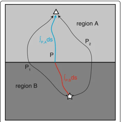
Here, we derive Eqs. (2) and (3) from the main text. The derivation is adapted in part from Snieder (2006).
The travel time tP of a seismic wave that propagates along a pathPis given by
tP¼ Z
P
1
vð Þr ds; ðA1Þ
where v(r) is the reference velocity at position r. We consider that the whole space is divided into regions A and B, as shown in Figure 11 of Appendix. Although the whole space is separated vertically in Figure 11 of Appendix for convenience, the following derivation holds for arbitrary separations. Assuming that the velocity of the medium is perturbed by a constant ratio δv0/v (|δv0/v| < < 1) in region A, we
de-fine a velocity perturbation function δvA(r) as
δvAð Þ ¼r δv0
v vð Þr inside region A 0 inside region B
(
: ðA2Þ
The travel time shift τP,A due to this velocity perturb-ation is given by
tPþτP;A ¼ Z
P
1
vð Þ þr δvAð Þrds≈ Z
P;A
1
vð Þr −
1
vð Þr δv0
v
ds
þ
Z
P;B
1
vð ÞrdsτP;A≈−
δv0
v
Z
P;A
1 vð Þr ds;
ðA3Þ
where the path integrals in regions A and B satisfy
Z
P;A
⋯ ð Þdsþ
Z
P;B
⋯ ð Þds¼
Z
P
⋯
ð Þds: ðA4Þ
The change in pathPdue to the velocity perturbation is negligible because the magnitude of the velocity per-turbation is much smaller than the reference velocity. In the same way, the travel time shift τP,B due to the vel-ocity perturbation function
δvBð Þ ¼r
0 inside region A
δv0
v vð Þr inside region B
(
ðA5Þ
is given by
τP;B≈−δv0
v
Z
P;B
1
vð Þr ds: ðA6Þ
Using Eqs. (A1), (A3), and (A6), we obtain
τP;AþτP;B≈−δv0
v
Z
P
1
vð Þr ds¼−
δv0
v tP: ðA7Þ
We now consider that the velocity of the medium is perturbed by constant ratios cAδv0/vand cBδv0/v in re-gions A and B, respectively, where cA and cB are arbi-trary constants that satisfy |cAδv0/v| < < 1 and |cBδv0/v| < < 1, respectively. The travel time shift due to these vel-ocity perturbations is given by
τP;cAAþcBB≈−cA δv0
v
Z
P;A
1 vð Þrds−cB
δv0
v
Z
P;B
1 vð Þr ds ¼cAτP;AþcBτP;B:
ðA8Þ
Because the observed wavefield is represented as a super-position of the waves that propagate along all possible paths distributed in a space (Piin Figure 11 of Appendix), the observed travel time shiftτof the wavefield is given by the weighted average of the travel time shifts for all waves (Snieder 2006), as follows:
region A
region B
P
P,B
ds
P,Ads
P
1P
2Fig. 11Schematic illustration that describes the separation of the whole medium into regions A and B. The curves Pirepresent paths
along which seismic waves propagate, whereiindicates the path number.∫P,Adsand∫P,Bdsare integrals along path P that pass
τ¼
X PτPIP X
PIP
; ðA9Þ
where IP is the intensity of the wave that propagates
along pathP.Using Eqs. (A7), (A8), and (A9), we obtain
τAþτB¼
X
P τP;AþτP;B
IP X
PIP
¼−δv0
v
X PtPIP X
PIP
¼−δv0
v t; ðA10Þ
and
τcAAþcBB ¼ X
PτP;cAAþcBBIP X
PIP≈cA X
PτP;AIP X
PIPþcB X
PτP;BIP X
PIP¼cAτAþcBτB:
ðA11Þ
Using Eqs. (A10) and (A11), we obtain
τcAAþcBBt ¼cAτAþcBτBt
¼−ð1−αÞcAδv0
v −α
cBδv0
v ; ðA12Þ
where
α¼ τB
τAþτB: ðA13Þ
In the main text, we regardedτA andτB as travel time
shifts due to 3% partial velocity reductions in the shallow (region A) and deep (region B) zones, respectively, and regardedcAδv0/vandcBδv0/vas the true relative velocity changes in the shallow and deep zones, respectively. We also consider that the apparent relative velocity change obtained from the Hi-net ACF is measured using the stretching technique, which implicitly uses
ΔV
V Hi¼−τcAAþcBBt: ðA14Þ
From Eqs. (A12), (A13), and (A14), we obtain Eqs. (2) and (3) in the main text.
Abbreviations
ACF:Autocorrelation function; DCW: Deconvolved waveform; FDM: Finite difference method; Hi-net: High-sensitivity seismograph network of Japan; KiK-net: Kiban Kyoshin strong-motion seismograph network of Japan; MDS: Maximum dynamic strain; NIED: National Research Institute for Earth Science and Disaster Resilience, Japan; PGV: Peak ground velocity; SVSC: Static volumetric strain change; TOE: Third-order elastic constants
Acknowledgements
We thank the Ministry of Land, Infrastructure, Transport and Tourism, Japan, for allowing us to use their streamflow data. Dr. T. Yano provided the relocated aftershock event catalog. We also thank Dr. T. Tanimoto, editor of
Progress in Earth and Planetary Science, and Dr. C. Hadziioannou and one anonymous reviewer for their thoughtful comments that improved the manuscript. Seismic Analysis Code (SAC; Goldstein and Snoke 2005) and
Generic Mapping Tools (GMT; Wessel et al. 2013) were used for signal processing and for constructing figures, respectively.
Funding Not applicable.
Authors’contributions
KS analyzed the data and drafted the manuscript. TS, TU, and KS provided many comments and suggestions to improve the manuscript. All authors read and approved the final manuscript.
Competing interests
The authors declare that they have no competing interests.
Received: 21 April 2016 Accepted: 7 November 2016
References
Aki K, Richards PG (2002) Quantitative seismology. Univ. Sci. Books, Sausalito, p 700
Beresnev IA, Wen KL (1996) Nonlinear soil response—a reality? Bull Seismol Soc Am 86(6):1964–1978
Brechet Y, Estrin Y (1994) The effect of strain rate sensitivity on dynamic friction of metals. Scr Metall Mater 30(11):1449–1454
Brenguier F, Campillo M, Hadziioannou C, Shapiro NM, Nadeau RM, Larose E (2008) Postseismic relaxation along the San Andreas Fault at Parkfield from continuous seismological observations. Science 321:1478–1481. doi:10.1126/ science.1160943
Brenguier F, Campillo M, Takeda T, Aoki Y, Shapiro NM, Briand X, Emoto K, Miyake H (2014) Mapping pressurized volcanic fluids from induced crustal seismic velocity drops. Science 345(6192):80–82
Burtin A, Bollinger L, Vergne J, Cattin R, Nábělek JL (2008) Spectral analysis of seismic noise induced by rivers: a new tool to monitor spatiotemporal changes in stream hydrodynamics. J Geophys Res 113:B05301. doi:10.1029/ 2007JB005034
Claerbout JF (1968) Synthesis of a layered medium from its acoustic transmission response. Geophysics 33(2):264–269
Fujiwara H, Kawai S, Aoi S, Morikawa N, Senna S, Kudo N, Ooi M, Hao KX-S, Hayakawa Y, Toyama N, Matsuyama H, Iwamoto K, Suzuki H, Liu Y (2009) A study on subsurface structure model for deep sedimentary layers of Japan for strong-motion evaluation. Technical Note of the National Research Institute for Earth Science and Disaster Prevention 337:260
Gardner GHF, Gardner LW, Gregory AR (1974) Formation velocity and
density—the diagnostic basics for stratigraphic traps. Geophysics 39:770–780. doi:10.1190/1.1440465
Gassenmeier M, Sens-Schönfelder C, Eulenfeld T, Bartsch M, Victor P, Tilmann F, Korn M (2016) Field observations of seismic velocity changes caused by shaking-induced damage and healing due to mesoscopic nonlinearity. Geophys J Int 204(3):1490–1502. doi:10.1093/gji/ggv529
Goldstein P, Snoke A (2005) SAC availability for the IRIS community, Incorporated Institutions for Seismology Data Management Center Electronic Newsletter. http://ds.iris.edu/ds/newsletter/vol7/no1/sac-availability-for-the-iris-community/
Hadziioannou C, Larose E, Coutant O, Roux P, Campillo M (2009) Stability of monitoring weak changes in multiply scattering media with ambient noise correlation: laboratory experiments. J Acoust Soc Am 125(6):3688–3695 Hobiger M, Wegler U, Shiomi K, Nakahara H (2012) Coseismic and postseismic
elastic wave velocity variations caused by the 2008 Iwate-Miyagi Nairiku earthquake, Japan. J Geophys Res 117:B09313. doi:10.1029/2012JB009402 Holliger K, Levander AR (1992) A stochastic view of lower crustal fabric based on
evidence from the Ivrea zone. Geophys Res Lett 19(11):1153–1156 Kanu C, Snieder R (2015) Time-lapse imaging of a localized weak change with
multiply scattered waves using numerical-based sensitivity kernel. J Geophys Res Solid Earth 120(8):5595–5605
Maeda T, Obara K, Yukutake Y (2010) Seismic velocity decrease and recovery related to earthquake swarms in a geothermal area. Earth Planets Space 62: 685–691. doi:10.5047/eps.2010.08.006
Meier U, Shapiro NM, Brenguier F (2010) Detecting seasonal variations in seismic velocities within Los Angeles basin from correlations of ambient seismic noise. Geophys J Int 181(2):985–996
Murnaghan FD (1967) Finite deformation of an elastic solid. Dover, New York, p. 124
Nakata N, Snieder R (2012) Time-lapse change in anisotropy in Japan’s near surface after the 2011 Tohoku-Oki earthquake. Geophys Res Lett 39:L11313 Obermann A, Planès T, Larose E, Sens-Schönfelder C, Campillo M (2013a) Depth
sensitivity of seismic coda waves to velocity perturbations in an elastic heterogeneous medium. Geophys J Int 194(1):72–382. doi:10.1093/gji/ggt043 Obermann A, Planès T, Larose E, Campillo M (2013b) Imaging preeruptive and
coeruptive structural and mechanical changes of a volcano with ambient seismic noise. J Geophys Res: Solid Earth 118(12):6285–6294
Okada Y (1992) Internal deformation due to shear and tensile faults in a half-space. Bull Seism Soc Am 82(2):1018–1040
Okada Y, Kasahara K, Hori S, Obara K, Sekiguchi S, Fujiwara H, Yamamoto A (2004) Recent progress of seismic observation networks in Japan―Hi-net, F-net, K-net and KiK-K-net―. Earth Planets Space 56:15–28
Pacheco C, Snieder R (2005) Time-lapse travel time change of multiply scattered acoustic waves. J Acoust Soc Am 118(3):1300–1310
Pacheco C, Snieder R (2006) Time-lapse traveltime change of singly scattered acoustic waves. Geophys J Int 165(2):485–500
Poupinet G, Ellsworth WL, Frechet J (1984) Monitoring velocity variations in the crust using earthquake doublets: an application to the Calaveras fault, California. J Geophys Res 89:5719–5731. doi:10.1029/JB089iB07p05719 Prioul R, Bakulin A, Bakulin V (2004) Nonlinear rock physics model for estimation
of 3D subsurface stress in anisotropic formations: theory and laboratory verification. Geophysics 69(2):415–425
Rivet D, Campillo M, Shapiro NM, Cruz-Atienza V, Radiguet M, Cotte N, Kostoglodov V (2011) Seismic evidence of nonlinear crustal deformation during a large slow slip event in Mexico. Geophys Res Lett 38:L08308. doi:10. 1029/2011GL047151
Rubinstein JL, Beroza GC (2004) Nonlinear strong ground motion in the ML5.4
Chittenden earthquake: evidence that preexisting damage increases susceptibility to further damage. Geophys Res Lett 31:L23614
Rubinstein JL, Beroza GC (2005) Depth constraints on nonlinear strong ground motion from the 2004 Parkfield earthquake. Geophys Res Lett 32:L14313. doi: 10.1029/2005GL023189
Sánchez-Sesma FJ, Campillo M (2006) Retrieval of the Green’s function from cross correlation: the canonical elastic problem. Bull Seismol Soc Am 96(3):1182–1191 Sato H, Fehler MC, Maeda T (2012) Seismic wave propagation and scattering in
the heterogeneous Earth. Springer, Berlin Heidelberg
Sawazaki K, Sato H, Nishimura T, Nakahara H (2009) Time-lapse changes of seismic velocity in the shallow ground caused by strong ground motion shock of the 2000 Western-Tottori earthquake, Japan, as revealed from coda deconvolution analysis. Bull Seismol Soc Am 99:352–366
Sawazaki K, Kimura H, Shiomi K, Uchida N, Takagi R, Snieder R (2015) Depth-dependence of seismic velocity change associated with the 2011 Tohoku earthquake, Japan, revealed from repeating earthquake analysis and finite-difference wave propagation simulation. Geophys J Int 201(2):741–763 Sens-Schönfelder C, Wegler U (2006) Passive image interferometry and seasonal
variations of seismic velocities at Merapi Volcano, Indonesia. Geophys Res Lett 33:L21302. doi:10.1029/2006GL027797
Snieder R (2006) The theory of coda wave interferometry. Pure Appl Geophys 163(2-3):455–473
Snieder R,Şafak E (2006) Extracting the building response using seismic interferometry: theory and application to the Millikan Library in Pasadena, California. Bull Seism Soc Am 96(2):586–598
Takagi R, Okada T, Nakahara H, Umino N, Hasegawa A (2012) Coseismic velocity change in and around the focal region of the 2008 Iwate-Miyagi Nairiku earthquake. J Geophys Res 117:B06315. doi:10.1029/2012GL051342 TenCate JA, Smith E, Guyer RA (2000) Universal slow dynamics in granular solids.
Phys Rev Lett 85(5):1020–1023
Ueno T, Saito T, Shiomi K, Enescu B, Hirose H, Obara K (2012) Fractional seismic velocity change related to magma intrusions during earthquake swarms in the eastern Izu peninsula, central Japan. J Geophys Res 117:B12305
Ueno T, Saito T, Shiomi K, Haryu Y (2015) Monitoring the instrument response of the high-sensitivity seismograph network in Japan (Hi-net): effects of response changes on seismic interferometry analysis. Earth Planets Space 67(1):1–10
Weaver RL, Hadziioannou C, Larose E, Campillo M (2011) On the precision of noise correlation interferometry. Geophys J Int 185(3):1384–1392 Wegler U, Sens-Schönfelder C (2007) Fault zone monitoring with passive image
interferometry. Geophys J Int 168(3):1029–1033. doi:10.1111/j.1365-246X.2006. 03284.x
Wessel P, Smith WHF, Scharroo R, Luis JF, Wobbe F (2013) Generic Mapping Tools: improved version released, EOS Trans. AGU 94:409–410
Yang W, Ge H, Wang B, Hu J, Yuan S, Qiao S (2014) Active source monitoring at the Wenchuan fault zone: coseismic velocity change associated with aftershock event and its implication. Earthq Sci 27(6):599–606. doi:10.1007/ s11589-014-0101-0
Yarai H, Yamada S, Morishita Y, Kobayashi T, Tobita M (2015) Postseismic deformation of the 2014 Northern Nagano Prefecture Earthquake. 2015 Seism Soc Japan Fall Meeting S03:P15
Submit your manuscript to a
journal and benefi t from:
7Convenient online submission
7Rigorous peer review
7Immediate publication on acceptance
7Open access: articles freely available online
7High visibility within the fi eld
7Retaining the copyright to your article