R E S E A R C H
Open Access
Developing GIS-based eastern equine
encephalitis vector-host models
in Tuskegee, Alabama
Benjamin G Jacob
1*, Nathan D Burkett-Cadena
2, Jeffrey C Luvall
3, Sarah H Parcak
4, Christopher JW McClure
5,
Laura K Estep
5, Geoffrey E Hill
5, Eddie W Cupp
6, Robert J Novak
1, Thomas R Unnasch
7Abstract
Background:A site near Tuskegee, Alabama was examined for vector-host activities of eastern equine
encephalomyelitis virus (EEEV). Land cover maps of the study site were created in ArcInfo 9.2
®
from QuickBird data encompassing visible and near-infrared (NIR) band information (0.45 to 0.72μm) acquired July 15, 2008.Georeferenced mosquito and bird sampling sites, and their associated land cover attributes from the study site, were overlaid onto the satellite data. SAS 9.1.4
®
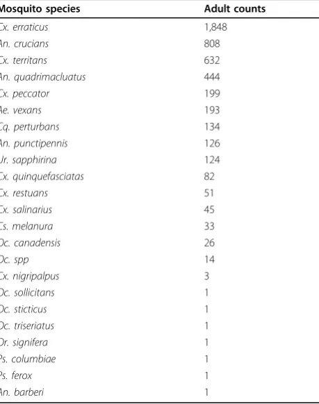
was used to explore univariate statistics and to generate regression models using the field and remote-sampled mosquito and bird data. Regression models indicated thatCulex erracticusand Northern Cardinals were the most abundant mosquito and bird species, respectively. Spatial linear prediction models were then generated in Geostatistical Analyst Extension of ArcGIS 9.2®
. Additionally, a model of the study site was generated, based on a Digital Elevation Model (DEM), using ArcScene extension of ArcGIS 9.2®
.Results:For total mosquito count data, a first-order trend ordinary kriging process was fitted to the semivariogram at a partial sill of 5.041 km, nugget of 6.325 km, lag size of 7.076 km, and range of 31.43 km, using 12 lags. For total adultCx. erracticuscount, a first-order trend ordinary kriging process was fitted to the semivariogram at a partial sill of 5.764 km, nugget of 6.114 km, lag size of 7.472 km, and range of 32.62 km, using 12 lags. For the total bird count data, a first-order trend ordinary kriging process was fitted to the semivariogram at a partial sill of 4.998 km, nugget of 5.413 km, lag size of 7.549 km and range of 35.27 km, using 12 lags. For the Northern Cardinal count data, a first-order trend ordinary kriging process was fitted to the semivariogram at a partial sill of 6.387 km, nugget of 5.935 km, lag size of 8.549 km and a range of 41.38 km, using 12 lags. Results of the DEM analyses indicated a statistically significant inverse linear relationship between total sampled mosquito data and elevation (R2 = -.4262; p < .0001), with a standard deviation (SD) of 10.46, and total sampled bird data and elevation (R2 = -.5111; p < .0001), with a SD of 22.97. DEM statistics also indicated a significant inverse linear relationship between total sampledCx. erracticusdata and elevation (R2= -.4711; p < .0001), with a SD of 11.16, and the total sampled Northern Cardinal data and elevation (R2 = -.5831; p < .0001), SD of 11.42.
Conclusion:These data demonstrate that GIS/remote sensing models and spatial statistics can capture
space-varying functional relationships between field-sampled mosquito and bird parameters for determining risk for EEEV transmission.
Introduction
Eastern equine encephalitis virus (EEEV) is the most dangerous endemic arbovirus in the United States. Up to 70% of symptomatic cases in humans are fatal [1],
and most survivors are permanently debilitated by neu-rologic sequelae [2]. Besides the endemic and economic burdens to humans, frequent equine cases and sporadic mass game bird die-offs are costly consequences of EEEV transmission [3-5]. Epornitics in wild birds are also dramatic consequences of EEEV [6], such as die-offs of the endangered whooping crane,Grus americana
[7]. Except in Florida [8,9], the ecology of EEEV is less * Correspondence: [email protected]
1
School of Medicine, Department of Infectious Diseases, University of Alabama at Birmingham, 845 19th Street South, Birmingham Alabama, USA, 35294
understood in the southeastern United States than in other endemic locations in the region. This disease is endemic in Alabama with viral activity varying between years. The summer of 2001 was a particularly active year for EEEV, with one human and over 30 veterinary cases in the central and southern regions of the state [10].
The mosquito speciesCuliseta melanurais generally believed to initiate EEEV transmission to wild birds [11,12]. Passerine birds are the major enzootic reser-voirs, and early transmission among the local avifauna is believed to be initiated by ornithophilic species, such as
Cs. melanura[11-13]. However, peaks in abundance of
Cs. melanura species do not correlate directly with peaks in EEEV transmission [14]. Differences in sampled abundance count data suggest that multiple mosquito species are necessary as vectors to account for large epi-zootics [11]. In addition toCs. melanura, several other mosquito species are likely involved as bridge vectors for EEEV transmission. These species include: Aedes vexans, Coquillettidia perturbans,Culex erraticus, while
Culex peccator, Culex territans and Uranotaenia sap-phirinaare suspected of circulating EEEV among rep-tiles and amphibians [15,16]. Of these previously listed species, it is suspected that Cx. erraticus is the most important EEEV bridge vector between birds and mam-mals in the mid-south, because of frequent virus isola-tions and its abundance in bottomland swamps, flood plains, permanent standing water, recreation areas near rivers or ponds, and water impoundments in Alabama and throughout the Tennessee Valley [10,17,18]. Under-standing the spatial distribution of this habitat-restricted species is valuable for predicting risk of EEEV infection for nearby human populations.
Despite the misnomer “equine,” EEEV transmission initiates in the avian cycle. Antibody prevalence in wild birds associated with freshwater swamps in Alabama range from 6-85% [19], which suggests that different bird species vary in attractiveness to mosquitoes and defensive behaviors against mosquito bites [20]. In Macon County, Alabama, avian species overrepresented in mosquito bloodmeals included: Yellow-Crowned Night-Heron, Carolina Chickadee, Great Blue Heron, Northern Mockingbird, and Wild Turkey [21]. There-fore, determining the spatial distribution of common bloodmeal hosts of mosquito vectors is a critical step to predicting early cycles of EEEV transmission.
Predicting foci of EEEV positive mosquitoes has been difficult, perhaps as a result of movement of human and horse populations and fluctuations in bird populations over the years [9]. Spatio-temporal distribution of arbo-viral vectors and hosts vary over short distances, based on differences in land cover and meteorological shifts. For example, human cases of West Nile Virus (WNV)
and St. Louis Encephalitis (SLE) clustered in urban/sub-urban areas in Georgia and Alabama [22,23]; whereas, EEEV transmission was restricted to freshwater swamps in Florida [9]. Compared to other arboviral diseases, EEEV transmission tends to be more spatially isolated [8,9], with the notable exception of the 1989 Atlantic and Gulf coast outbreaks, which caused 196 equine cases and 9 human cases [3]. Evidence for spatial isola-tion of EEEV foci include the lack of early warning of transmission with sentinel flocks and very low serocon-versions of both sentinel flocks (2%) and human popula-tions within EEEV foci (1.7%) [3,8,9,24], suggesting few asymptomatic cases. Therefore, untargeted or random interventions would be excessive and wasteful [25], as EEEV vectors and hosts are not randomly distributed.
Quantification of vector-host interactions, by incor-porating high resolution remotely sensed data in GIS, can help predict arbovirus transmission cycles by identi-fying site specific environmental predictors [25-32]. For example, in earlier research, Jacob et al. [31] found that land use land cover (LULC) change sites can aid in spa-tial prediction of human exposure toCulexmosquitoes using GIS-generated models. A LULC classification, based on Landsat-7 ETM+ data acquired in July 2003 and Landsat-5 TM data acquired in July 1991, was com-pared to the abundance of Culex restuans and Culex pipiens egg rafts in Urbana-Champaign, Illinois. Total LULC change, from 1991 to 2003 in the Urbana-Cham-paign study site, was relatively low (12.1%). The most frequent LULC category was maintained urban. The urban land cover was further subdivided by degree of tree canopy coverage using QuickBird visible and near infra-red (NIR) data, which revealed 73.3% of the urban area was in the category classified as high canopy cover-age, with 20% of the remotely stratified data categorized as moderate canopy coverage, and 6.7% as low coverage. The remote stratification of the urban land cover revealed that 83.3% egg raft distribution was in the high coverage areas [31].
variables [35]. Topographic derivatives generated from a DEM can also be calculated at different scales, using the linear interpolation technique built in GIS, which can accurately yield several catchment hydrological variables, including percent surface saturation and total surface runoff for identification of potential mosquito and avian sampling sites [33].
Vector-borne disease risk can also be modeled with high predictive accuracy by using geostatistical kriging algorithms in GIS. Kriging is equated with spatial opti-mal linear prediction, where the unknown random-pro-cess mean is estimated with the best linear unbiased estimator. Kriging field and remote-sampled mosquito and avian predictor variables require the use of various geostatistical techniques to interpolate the parameters of a random field (e.g., the elevation, z, of the landscape as a function of the geographic location, at an unsampled location from data at nearby sampled locations) [34]. Stochastic kriging can also be used to generate predic-tion of abundance and distribupredic-tion data, which can allow for numerical quantification of uncertainty esti-mates in arboviral explanatory covariates [31]. Addition-ally, predicting landscape classes in urban environments can reveal local spatial patterns of the physical and socio-economic factors hypothesized to be associated with arboviral transmission. For example, in northern California, kriging interpolation revealed thatCulex tar-salis was the most abundant species in ovitraps near agricultural sites; whereas, Cx. pipiens was clustered within residential areas [33].
The dynamics of transmission of any arthropod-borne infection is a complex function of many factors, which may include the intensity of infection in the vertebrate reservoir, the competence of the vector, and the degree of contact of the vector with the infected vertebrate host reservoir [37]. Thus, generating models of EEEV, using field and remote-sampled mosquito and avian data, is essential to understanding the ecology of EEEV and for developing effective means to control outbreaks. GIS/ remote sensing and spatial statistics can map interac-tions between arthropod mosquito vectors and avian amplification host populations, which can aid in spatially targeting high density foci of mosquito and avian sam-pling sites [31]. Treatments or habitat perturbations should be based on the surveillance of the most produc-tive areas of an ecosystem [25]. Therefore, the objecproduc-tives of this research were: a) to generate multiple regression models to determine predictors associated with the sampled mosquito and avian data; (b) to develop spatial linear prediction models of potential avian and mosquito sampled sites; and, c) to construct a DEM to identify terrain covariates associated with sampled mosquito and bird data in Tuskegee, Alabama.
Materials and methods
Study Site
The study site is located in the Tuskegee National Forest in Macon County, Alabama. Since the site was abandoned in the 1900s, it has undergone extensive re-encroachment of forest over depleted farmland and is characterized by forested bottomland wetlands [10]. The center of Tuske-gee, AL is located approximately 3 km from the edge of the study site, an urban center with a human population density of 3,700 persons/km2http://factfinder.census.gov. The western edge of the sampling grid abutted the City Lake, east of the center of Tuskegee, an area with a human population density of 1,100-1,600 persons/km2. The north-west portion of the sampling grid also overlapped with populated areas northeast of Tuskegee and north of high-ways US-29/AL-81, with a human population density of also 1,100-1,600 persons/km2. The geographic coordinates of the centroid of the sampling grid were 85.644444 by 32.432494 decimal degrees. The central and southern por-tions of the sampling grid had a human population density of 80 persons/km2, and the eastern edge had a human population density of 0-50 persons/km2.
Collections
Remote sensing data
QuickBird data http://www.digitalglobe.com encompass-ing the visible and near infra-red (NIR) bands was acquired on July 15, 2008 for the study site. QuickBird multispectral products provided four discrete non-over-lapping spectral bands covering a range from 0.45 to 0.72 μm, with an 11-bit collected information depth. The spatial resolution of the data was 0.61m. The clear-est, cloud-free imagery available of the contiguous sub-areas of the study site was used to identify mosquito and wild bird sampling sites.
Base mapping
Base maps of major roads and hydrological networks were created using ArcInfo 9.2
®
(Environmental Systems Research Institute, Redlands, California) from differen-tially corrected global positioning system (DGPS) ground coordinates. In this research, fixed surveillance sites were geocoded using a CSI-Wireless (DGPS) Max receiver with a real-time Omni Star L-Band satellite signal, which has a positional accuracy of 0.179 m (+/0.392 m) [31]. A 10m × 10 m grid-based matrix was overlaid on the base maps of the study site, in ArcInfo 9.2®
to generate effi-cient spatial sampling units. A unique identifier was placed in each grid cell. For remote identification of arbo-viral mosquito and avian habitats, the first step is often to construct a discrete tessellation of the region [41-48].Regression analyses
A linear regression, with statistical significance, was determined by a 95% confidence level and used to ascer-tain whether the proportions of sampled mosquito data differed by grid cell. The linear regression model assumed a random sample betweenYi, (sampled mosquito habitat count data), the regress and regressorsXi1, ...Xip. A dis-turbance term εi, which was a random variable, was added to this assumed relationship to capture the influ-ence of all habitat parameters sampled onYiother than
Xi1, ...Xip. The random error term,ε, in a regression ana-lysis of field and remote-sampledCulexaquatic model, is typically assumed to be normally distributed with mean zero and variances2 [31]. Statistical characteristics of the sampled data were examined in PROC UNIVARIATE. The PLOT option in the PROC UNIVARAITE statement generated histograms and boxplots. The NORMAL option was used to test whether the field and remote-sampled parameters had a normal distribution. The regression analyses was performed using PROC REG. The multiple linear regression model was:
Yi =0+1Xi1+2Xi2++pXip+i, i=1,, .n
It was important to distinguish the model in terms of random variables and the observed values of the random
variables. Thus, we determined p+ 1 parametersb0, ..., bp. In order to estimate the sampled mosquito aquatic habitat parameters, it was useful to use the matrix nota-tion Y = Xb + ε, where Y was a column vector that included the mosquito count values of Y1, ...,Yn, which included the unobserved stochastic componentsε1, ...,εn and the matrix X. This matrix was the observed mos-quito aquatic habitat parameter values of the regressors expressed as:
X
x x
x x
x x
p p
n np
= ⎛
⎝ ⎜ ⎜ ⎜ ⎜⎜
⎞
⎠ ⎟ ⎟ ⎟ ⎟⎟ 1
1
1
11 1
21 2
1
.
In this research, X included a column that did not vary across the sampled mosquito data, which was used to represent the intercept termb0.
The ecological-sampled data was log-transformed before analyses to normalize the distribution and minimize stan-dard error. Multicollinearity diagnostics from the COLLIN option in SAS
®
were estimated. Residual-based diagnostics for univariate and multivariate conditional heteroscedastic models, previously constructed from clustering field and remote-sampled mosquito habitat parameter estimates have revealed that errors in variance uncertainty estima-tion can substantially alter numerical predicestima-tions models due to multicollinearity [31]. The SAS COLLIN option produced eigenvalues and condition index, as well as pro-portions of variances with respect to individual-sampled predictor variables in the model. The conditional index scores indicated no significant multicollinearity with the model. It was hypothesized, however, that serial correla-tion could be a major source of time-varying heterogene-ity. In this research, the Durbin-Watson statistic was used to detect the presence of autocorrelation in the residuals from the regression analysis. The Durbin-Watson can test for first-order serial correlation [49]. Usually, the Durbin-Watson statistic is used to test the null hypothesisH0:1= 0 againstH1:1> 0 [49]. The generalized Durbin-Watson statistic is written as:DW uA A u
u u j
j j
= ˆ ′′ ˆ
ˆ ˆ
where ˆu is a vector of OLS residuals andAjis a (T-j) ×Tmatrix. In this research, the generalized Durbin-Wat-son statistic DWjwas rewritten as:
DW Y MA A MY
Y MY
Q A A Q j
j j j j
= ′ ′
′ =
′ ′ ′ ′
( 1 1)
The marginal probability for the Durbin-Watson sta-tistic was:
Pr(DWj <c)=Pr(h<0)
whereh=h’(Q’1A’jAjQ1-cI)h.
Thep-value, or the marginal probability, for the gen-eralized Durbin-Watson statistic, was computed by numerical inversion of the characteristic function j(u) of the quadratic formh=h’(Q’1A’jAjQ1- cI)h. The tra-pezoidal rule approximation to the marginal probability Pr(h< 0) was:
Pr( )
Im[ (( ) )]
( )
( ) ( )
h
k
k
K k
K
I T
< = − +
+ + +
=
∑
0 1
2
1 2 1 2 0
Δ
Δ
E E
where IM[j(·)] was part of the characteristic function and EI(Δ) and ET(K) were integration and truncation errors, respectively. The trapezoidal rule is a way to cal-culate the definite integral [49]. A numerically efficient algorithm was used to quantify the autocorrelated com-ponents in the regression model, which required O(N) operations for evaluation of the characteristic functionj (u). The characteristic function was denoted as:
( ) |u I−2iu(Q A A Q′ ′1 j j 1−cIN k− ) |−1 2/
|V|−1 2/ |X V′ −1X|−1 2/ |X X′ |1 2/ where
V = +(1 2iuc)I−2iuA A and ′j j i= −1.
By applying the Cholesky decomposition to the com-plex matrix V, we obtained the lower triangular matrix
Gthat satisfied V =GG’. Cholesky decomposition is a decomposition of a symmetric, positive-definite matrix into the product of a lower triangular matrix and its conjugate transpose [49]. The characteristic function was evaluated in O(N) operations by using the following formula:
( ) |u =G| |−1 X*′X*|−1 2/ |X X′ |1 2/
whereX* =G-1X.
We tested for serial correlation with lagged dependent variables in the model (Appendix a). When regressors contain lagged dependent variables, the Durbin-Watson statistic (d1) for the first-order autocorrelation is biased toward 2 and has reduced power [50]. If the Durbin-Watson statistic is substantially less than 2, there is evi-dence of positive serial correlation [49]. In AUTOREG,
two alternative statistics (Durbinhandt) can be used to test for time varying residuals that are asymptotically equivalent [50]. In this research, we used the hstatistic, which was written as:
h=ˆ N / (1−NVˆ )
where
ˆ ˆ ˆ / ˆ
=
∑
= V Vt t−∑
t= Vt N tN
1 1 2
2 , and Vˆ was the least
squares variance estimate for the coefficient of the lagged dependent variable.
In PROC AUTOREG, an estimation method was used to generate an autoregressive error model using the Yule-Walker (YW) method. The YW method can be considered as generalized least squares using the OLS residuals to estimate the covariances across observation [49]. In this research, we letrepresent the vector of autoregressive parameters,= (1,2,...,m)’, and we let the variance matrix of the error vector beν= (ν1, ...,νN)’beΣ,E(νν’=
Σ=s2V. If the vector of autoregressive parametersis known, the matrixVcan be computed from the autore-gressive parameters;Σis thens2V[49]. GivenΣ, the effi-cient estimates of regression parametersbwere computed using generalized least squares (GLS). The GLS estimates then yielded the unbiased estimate of the variances2.
The YW method alternated estimation ofbusing gen-eralized least squares with estimation of , which the YW equations applied to the sample autocorrelation function. The YW method started by forming the OLS estimate of b. Next, was estimated from the sample autocorrelation function of the OLS residuals by using the YW equations. Then V was estimated from, and
Σ was generated fromVand the OLS parameters ofs2. The autocorrelation corrected estimates of the regres-sion parameters,b, were then computed using GLS and the estimated matrix. The YW equations, solved to obtain ˆ and a preliminary estimate of s2, were Rj= -r. In this research, we used the equation r= (r1...,rm)’, whenriwas the lagisample autocorrelation. The matrix
R was the Toeplitz matrix, whose i, jth element was
r|i-j|. Toeplitz matrix is a matrix in which each descend-ing diagonal from left to right is constant [49]. We spe-cified a subset model. Only the rows and columns ofR andrcorresponding to the subset of lags specified were used. The BACKSTEP option was specified for purposes of significance testing. The matrix [Rr] was treated as a sum-of-squares-and-cross products matrix arising from a simple regression with N - k observations, where k was the number of estimatedCx. erraticushabitat para-meters in the model.
Digital elevation model
ArcScene extension of ArcGIS
®
. The DEM used in this research was a raster representation of a continuous sur-face, originating from the Shuttle Radar Topography Mission (SRTM) which had a spatial resolution of 92 m. The probability distribution of the soil moisture deficit, i.e., statistics of topography, was generated from the DEM data by using a multidirectional flow routing algo-rithm. The purpose of DEM construction was to extract topographic parameters that may have been associated with the field and remote-sampled EEEV mosquito and bird covariates. A flow apportioning algorithm can delineate a realistic channel network for quantifying hydrogeomorphic properties of simulated drainage pat-terns using DEMs for identifying floodwater mosquitoes [35].Spatial analyses
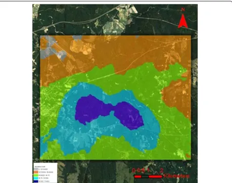
Kriging models were generated using all sampled abun-dance count data in Geostatistical Analyst Extension of ArcGIS 9.2
®
. However, based on the evidence that Cx. erraticus is likely the primary bridge vector of EEEV in Tuskegee [10] and was the most abundant species sampled in the study site, it was selected for the inde-pendent kriging analyses (Table 1). Also, kriging ana-lyses were run for total abundance counts of the sampled bird data in Tuskegee, in 2007. Frompreliminary data analyses, it was determined that North-ern Cardinals were the most abundant avian species in the study site (Table 2). Therefore, a kriged model was generated using the Northern Cardinal data sample points. All the models were created in the ArcGIS 9.3
®
Geostatistical Analyst Extension.Spatial linear prediction was performed using ordinary kriging. Geostatistical techniques were used to interpo-late the values Z(x0), at a sampled mosquito or bird habitatZ(x), for unobserved sampling sitesx0 and zi= Z (xi), i = 1... n, using data sampled at nearby sampled habitat locations (x1,...xn). The kriged-based algorithm computed the best linear unbiased estimator, Ž(xo) ofZ (x0), for the sampled habitat data, based on a stochastic model of the spatial dependence quantified by the vario-gram g(x, y), by expectationμ(x) = E[Z(x)], and by the covariance functionc(x,y) of the random field. In this research, the kriging estimator was given by a linear combination:
ˆ ( ) ( ) ( )
Z xo w x Z xi o i i
n
= =
∑
1(2:1)
for analyzing the sampled data; where, zi =Z(xi) was the weights while wi(xo) andi= 1...nwas the variance used to minimize any biased condition [35]. The depen-dent variables were the sampled adult count of mosqui-toes or bird data, which were transformed to fulfill the diagnostic normality test prior to performing the kri-ging. The kriging weights were then used to fulfill the unbiasedness condition in the spatial interpolation of the ecological-dependent variables using:
i i
n
=
∑
=1
1 (2:2)
Table 1 Adult mosquito counts for the Tuskegee study site
Mosquito species Adult counts
Cx. erraticus 1,848
An. crucians 808
Cx. territans 632
An. quadrimacluatus 444
Cx. peccator 199
Ae. vexans 193
Cq. perturbans 134
An. punctipennis 126
Ur. sapphirina 124
Cx. quinquefasciatas 82
Cx. restuans 51
Cx. salinarius 45
Cs. melanura 33
Oc. canadensis 26
Oc. spp 14
Cx. nigripalpus 3
Oc. sollicitans 1
Oc. sticticus 1
Oc. triseriatus 1
Or. signifera 1
Ps. columbiae 1
Ps. ferox 1
An. barberi 1
Table 2 Bird counts for the Tuskegee study site
Species Abundance (% of count)
Northern cardinal 119 (37.6) Carolina wren 77 (20.5) Red-eyed vireo 51 (8.2) Indigo bunting 50 (8.0) Tufted titmouse 36 (5.8) White-eyed vireo 35 (5.6) Acadian flycatcher 31 (5.0) Red-bellied woodpecker 14 (2.3) American crow 14 (2.3)
Blue jay 13 (2.1)
which was given by the ordinary kriging equation sys-tem:
1 1 1 1
1 1 1 n n
n n n
x x x x
x x x x
⎛ ⎝ ⎜ ⎜ ⎜ ⎜⎜ ⎞ ⎠ ⎟ ⎟ ⎟ ⎟⎟ = ( , ) ( , ) ( , ) ( , )) ( , ) ( , ) * * 1
1 1 0 1
1 1 ⎛ ⎝ ⎜ ⎜ ⎜ ⎜⎜ ⎞ ⎠ ⎟ ⎟ ⎟ ⎟⎟ ⎛ ⎝ ⎜ ⎜ ⎜ ⎜ ⎜ ⎞ ⎠ ⎟ ⎟ ⎟ ⎟ ⎟ − x x
xn x
The additional parameterμwas a Lagrange multiplier used in the minimization of the kriging error k2( )x to honor the unbiased condition in the ecological dataset [51]. The ordinary kriging was given by:
var( ( ) ( ))
( , ) ( , ) ( , ) * * * *
Z x Z x
x x x x x x n − = ⎛ ⎝ ⎜ ⎜ ⎜ ⎜ ⎜ ⎞ ⎠ ⎟ ⎟ ⎟ ⎟ ⎟
1 1 1
1 ( , ) ( , ) ( , ) ( , x x
x x x x
x
n
n n n
1 1 1 1 1 1
1 1 0
⎛ ⎝ ⎜ ⎜ ⎜ ⎜⎜ ⎞ ⎠ ⎟ ⎟ ⎟ ⎟⎟ − xx
xn x * * ) ( , ) 1 ⎛ ⎝ ⎜ ⎜ ⎜ ⎜ ⎜ ⎞ ⎠ ⎟ ⎟ ⎟ ⎟ ⎟
and the interpolation was given by:
ˆ ( *)
( ) ( ) Z x Z x Z x n n = ⎛ ⎝ ⎜ ⎜ ⎜ ⎞ ⎠ ⎟ ⎟ ⎟ ′ ⎛ ⎝ ⎜ ⎜ ⎜ ⎞ ⎠ ⎟ ⎟ ⎟ 1 1
with the error variables quantified using:
var Z x Z x
x x
x x
n n
ˆ ( *) ( *)
( , *) ( , *) −
(
)
= ⎛ ⎝ ⎜ ⎜ ⎜ ⎜⎜ ⎞ ⎠ ⎟ ⎟ ⎟ ⎟⎟ ′ ⎛ 1 1 1 ⎝⎝ ⎜ ⎜ ⎜ ⎜⎜ ⎞ ⎠ ⎟ ⎟ ⎟ ⎟⎟The semivariogram generated described the spatial dependence, between the sampled mosquito and bird parameters, as a function of the distance between the sampling sites. The semivariogram allowed for mosquito or bird abundance estimations at any point in the study site. The value of prevalence, Z, at the coordinate (x0,
y0) was estimated from thennearest sampling values: Zobs x y( ,1 1),Zobs x( 2,y2)Zobs x( n,yn)
by the linear formula:
ˆ ( , ) ( , )
Z x y a Zi obs x yi i i n 0 0 1 = =
∑
(2:3)Theaiwere found by the Lagrange multiplier l and solving the system:
ai hi j hi j n
i n ( ,)+ = ( , ), = ... =
∑
0 1 1under the constraint
ai i n = =
∑
1 1where hi, jdenoted the distance between any two mos-quito or bird sampled locations, located at (xi, yi), and (xj, yj), and hj,0 was the distance between the two mos-quito or bird sampled sites (x0, y0). The semivariance was defined as g (h) [50-53]. The magnitude of the semivariance in this research was dependent on the dis-tance between sampled mosquito or bird sites. Semivar-iance of the devSemivar-iance residuals of the mosquito and bird count data was calculated, and a variogram was con-structed to determine if there was evidence of latent spatial autocorrelation in the sampled data. The plot of the semivariances as a function of distance from a point is referred to as a semivariogram [53]. The empirical semivariogram and covariance can provide information on autocorrelation components in ecological-sampled datasets [49].
variance can represent noise characteristics in field and remote-sampled explanatory variables [31]. Additionally, a neighborhood distance search radius provided the mean standard errors of the interpolated values. Inter-polation accuracy can be measured by the natural loga-rithm of the mean squared interpolation error, which can reveal all main effects of parameter estimates, in an autoregressive model, while quantifying several covariate interaction terms [56-59].
Results
The regression models were able to classify sampled high and low abundance count habitats. Temperature had a significant association with Cx. erraticus adult abundance (p < 0.0002). The predictor variable precipi-tation also presented a significant relationship (p < 0.05). In this research, Durbin-Watson statistics were generated using the AUTOREG procedure in SAS
®
toestimate whether the OLS regression estimates indicated significant serial correlation with an estimated order of a lagged covariance of 1. The AUTOREG procedure corrected for serial correlation using the YW method. The Durbin-Watson statistic indicated that serial corre-lation was not significant in the YW corrected model. The YW estimates for the model indicated a R2 = 0.632, F statistics of 39.177, and Durbin-Watson score of 1.935. For total mosquito count data, a first-order trend ordinary kriging process was fitted to the semivario-gram at a partial sill of 5.041 km, nugget of 6.325 km, lag size of 7.076 km, and range of 31.43 km, using 12 lags. For total adult Cx. erracticus count, a first-order trend ordinary kriging process was fitted to the semi-variogram at a partial sill of 5.764 km, nugget of 6.114 km, lag size of 7.472 km, and range of 32.62 km, using 12 lags (Figure 1). For the total bird count data, a first-order trend ordinary kriging process was fitted to
the semivariogram at a partial sill of 4.998 km, nugget of 5.413 km, lag size of 7.549 km, and range of 35.27 km, using 12 lags. For the Northern Cardinal count data, a first-order trend ordinary kriging process was fitted to the semivariogram at a partial sill of 6.387 km, nugget of 5.935 km, lag size of 8.549 km, and a range of 41.38 km, using 12 lags (Figure 2). To evalu-ate the accuracy of the models, predictive mean stan-dard error distributions were generated, which revealed that all models were within normal statistical limita-tions (Table 3).
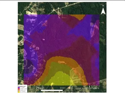
A DEM of the study site was generated in ArcGIS
®
(Figure 3). The minimum and maximum range of the elevation in the DEM models were calculated. Pearson’s correlation was used to evaluate the linear relationship between mosquito and bird count data and the sampled predictor variable elevation using the SRTM DEM. Results of the DEM analyses indicated a statistically sig-nificant inverse linear relationship between total sampled mosquito data and elevation in meters (m) (R2 = -.426; p < .0001), with a standard deviation (SD) of 104.6. The range of the elevation in the DEM had aFigure 2Predicted Northern Cardinal abundance count data in the Tuskegee study site using an Ordinary kriging algorithm.
Table 3 Residual model outputs from ordinary kriged models using mean error and root mean square error for the sampled mosquito and bird and count data in the Tuskegee study site.
Data Ordinary kriging mean error Ordinary kriging root mean square error
Total bird counts 0.055 1.821
Northern cardinal 0.163 1,642
Total mosquito counts -0.132 4.664
minimum value of 0 m, with a maximum value of 431 m. The results of the total sampled bird data and eleva-tion were (R2 = -.511; p < .0001), with a SD of 22.97. The range of the elevation in the DEM had a minimum value of 0 m, with a maximum value of 439 m. DEM statistics also indicated a significant inverse linear rela-tionship between total sampledCx. erracticusdata and elevation (R2 = -.471; p < .0001), with a SD = 111.6. The range of the elevation in the DEM had a minimum value of 0 m, with a maximum value of 487 m. The results of the total sampled Northern Cardinal data and elevation was (R2= -.583; p < .0001), with a SD = 114.2. The range of the elevation in the DEM had a minimum value of 0 m, with a maximum value of 501 m (Table 4). Discussion
Culex erraticuswas the most abundant mosquito species collected during this study in central Alabama bottom-land freshwater wetbottom-lands, which was ~6 km from the center of Tuskegee and ~1.5 km east of a populated area north of highways US-29/AL-81. This species pre-viously yielded the highest number of EEEV-infected pools in Tuskegee [21]. Habitat requirements of Cx. erraticusare shallow water [60-66], especially overgrown with surface plants or grassy margins, such as streams, lakes or impoundments [18]. This species may be col-lected in high numbers during hot weather, and even during drought, periods in July and August [10]. Blood-feeding hosts of Cx. erraticus include: birds (27-70%),
mammals (23-67%), and reptiles (2-20%), suggesting great host flexibility based on relative availability of hosts [16].
The bird communities present in the Tuskegee study site are typical of reforested areas of bottomland hard-wood [10]. The level of vector contact with different bird species in a given area is essential in identifying
Figure 3Digital Elevation Model (DEM) of the Tuskegee study site.
Table 4 Pearson correlation for mosquito and bird sampled data and the sampled predictor variable elevation in the Tuskegee study site.
Predictor variables Statistical tests Significance level
Elevation (m)
Total mosquito count data
Pearson Correlation
1 -.426
Sig. (2-tailed) <.0001 <.0001
N 141 118
Total bird count data Pearson Correlation
1 -.511
Sig. (2-tailed) <.0001 <.0001
N 141 118
Cx. erraticusdata Pearson Correlation
1 -.471
Sig. (2-tailed) <.0001 <.0001
N 141 118
Northern cardinal data Pearson Correlation
1 -.583
Sig. (2-tailed) <.0001 <.0001
those avian species that are most likely to serve as important amplifiers for arboviral enzootics [15]. Birds that frequent edge habitats are assumed most likely to transmit EEEV between localized pest mosquitoes and humans or horses [21]. Woodland and swamp birds spe-cies captured within an EEEV focus in Michigan had high antibody prevalence, but seroconversion of EEEV to other urban bird species in open areas increased dur-ing peak transmission to horses [65].
Previous research of EEEV in Alabama also has sug-gested the importance of hatch-year birds as catalysts for epidemic transmission. For example, wild birds involved in EEEV transmission in Alabama forested areas included: Yellow-Crowned Night-Heron, Carolina Chickadee, Northern Mockingbird and Great Blue Heron [21]; in Florida, the species were: Bluejay, North-ern Mockingbird, Rufus-Sided Towhee, Loggerhead Shike, Northern Cardinal, Cattle Egret and the game-birds Pheasant and Chukar Partridge [8]; and, in Louisi-ana, the species were: White-Throated Sparrow, Northern Cardinal, House Sparrow, Rufus-Sided Towhee, Carolina Chickadee and Yellow-Rumped War-bler [19]. Similarly, the House Sparrow is a primary vec-tor for WNV, EEEV and SLE in Louisiana [17]. Most of these listed birds are included on the Audubon Society checklist as very common species to Alabama for spring, summer and fall. Notably, birds involved in EEEV tend to be less urban than WNV/SLE avian hosts, though considerable host species overlap is apparent between diseases and between geographic regions [16]. Chicka-dees, Northern Cardinals, Tufted Titmice, Blue Jays, American Crows, Brown-Headed Cowbirds and Red-Billed Woodpeckers inhabit both wooded and human-populated areas [62]. American Crows may forage in wooded locations but roost at night in urban and subur-ban areas [8,46].
Culex erraticuswas the most common mosquito col-lected at the study site. Because of its density, it is likely that Cx. erraticusplays a major role in perpetuating EEEV transmission. Cx. erraticus is a member of the subgenusMelanoconion, a largely tropical group of mos-quitoes. Cx. erraticusis the most common member of that subgenous in the United States and is distributed throughout the eastern and the upper midwest and westward to California [16]. SinceCx. erraticusis a neo-tropical species which plays a major role in the trans-mission of EEEV in Tuskegee, the geographical distribution of EEEV in Alabama might resemble that seen in EEEV foci in tropical areas (e.g., South America). The probability that a mosquito will feed on a reservoir host is one of the most influential variables affecting the geographical distribution of an arthropod mosquito vec-tor [8]; therefore, determining spatial patterns of Cx. erraticushost preferences can play a significant role in
controlling the development of avian enzootics of EEEV in the Tuskegee study site.
Temperature and precipitation were important predic-tor variables in the regression model. Environmental conditions such as temperature, and precipitation, have an important effect on the distribution of the mosqui-toes that harbor arboviruses, thereby, influencing seaso-nal virus activity [3,10,11]. Previous regression aseaso-nalysis estimates derived from multiple field and remote-sampled predictor variables, collected from nine sites within Cook County, Illinois, revealed that adult Culex
population was positively associated with temperature [57]. The model output indicated that precipitation was negatively associated to mosquito abundance in 2002, 2003 and 2005 (P <0.05), but positively associated in 2004 (P <0.05). Naturally occurring outbreaks of EEEV are usually observed during periods of hot, rainy weather [3]. These weather conditions are ideal for expansion ofCs. melanuraand other mosquito popula-tions [63]. Outbreaks of EEEV in horses and humans are expected to occur from midsummer to late summer, with August being the peak month of incident cases in much of the United States [11]. An evaluation of EEEV in horses in Michigan, during five outbreaks between years 1972 and 1991, revealed an increase in Cs. mela-nura, Cq. perturbans, and Ae. vexansas vectors, wild and domestic birds as reservoir hosts, humans and com-mercial poultry flocks as incidental hosts, with an increase in the state-wide annual precipitation and an increase in region-specific precipitation [19]. Tempera-ture and precipitation is likely involved in early season enzootic transmission and late season epizootic amplifi-cation of the EEEV in wild bird populations at the Tus-kegee study site. It is possible that Cx. erraticus may become important as a bridge vector of EEEV in the southeastern United States, as human populations con-tinue to move closer to sylvatic sites, where populations of this mosquito have access to avian reservoirs and during specific time frames throughout the year, when there is fluctuation in meteorological variables. An important variable in the amplification from the enzoo-tic cycle of arboviral encephalitides is the degree of con-tact between avian hosts and mosquito vectors [21].
Culex erraticus has a minimally infection rate of 3.2, from mid-June to mid-September [16].
kilometers beyond their preferred habitats. Mosquito species differ in their overall preference for different classes of host (e.g., mammals versus birds versus rep-tiles), in the times of day that they are most active in seeking bloodmeals, and the heights at which they for-age [21]. Many of the mosquito hosts sampled were edge species, birds that are most common at the inter-face between forested and disturbed landscapes, such as cardinals, corvids, and parids. For example, Northern Cardinals were previously found six times more abun-dant in habitats surrounded by open space [11].
The semivariograms, generated in ArcGIS Spatial Analyst, modeled the structure of spatial variability in the field and remote-sampled Cx. erracticusand North-ern Cardinal habitat data. The semiovariograms were used to fit models of the spatio-temporal correlation of the sampled mosquito and bird parameters. The semi-variogram and covariance functions quantified the nearby habitats as a measure of the strength of statistical correlation and as a function of distance between sampled habitats. Linear predictors were generated by incorporating models of the covariance of the random function using a weighted moving average interpolation. The semivariogram of residuals from the regression models generated from the sampled covariates, with sta-tionary errors, were used to estimate the covariance structure of the underlying spatial structural processes in the data.
For prediction kriging, the bias of the semivariogram estimates induced, by using residuals instead of errors, has only a minor effect, as the bias is small for small lags [49]. However, in this research, error in the spatial covar-iance patterns generated from the estimated regression coefficients may have been quite substantial due to the excess land cover heterogeneity between the sampled habitats. To spatially analyze a mosquito vector, one must understand that insect populations are typically het-erogeneous in their spatial densities, responding to multi-variate habitat characteristics and environmental controls [25]. Additionally, kriging may not be widely used for predicting EEEV distribution at a local scale, because of the common finding of non-stationarity in ecological-sampled data. The violation of the stationarity assump-tion may affect the validity of kriged surfaces, since a common metric derived from the semivariogram is not enough to capture spatial variations in EEEV parameters observed at a local scale. The process of using kriged-based algorithms for mosquito and bird parameters may require estimation of the best model parameters, and an assessment of the resulting model accuracy, before it can be used as a predictive tool for evaluating EEEV mos-quito and bird habitat data. Diagnostic checking error residuals in an EEEV model may enable intervention efforts spatially targeting productive mosquito and bird
habitats based on field and remote-sampled data, by using the asymptotic distribution of parameter estimates from a residual autocovariance matrix.
The distribution of Northern Cardinals was interest-ing, as this species was by far the most abundant, preva-lent, and evenly distributed bird species detected in the Tuskegee study site. This species has also expanded range over the last century due to mild winter patterns and increased use of bird feeders for winter survival [11]. Despite the very high abundance of Northern Car-dinals, this species appeared only moderately attractive to host-seeking mosquitoes [10]. Northern Cardinals are common in both forest and urban habitats [19] Radio tracking data suggests that individual cardinals are highly territorial of small plots of land and do not typi-cally migrate more than 50 m from their roosts [14]. It is possible that the high abundance and prevalence of Northern Cardinals prevented smaller passerine EEEV hosts from reaching higher densities. The spatial pat-terns of total bird counts, Northern Cardinal counts, did not significantly differ; whereas, the spatial pattern of
Cx. erraticussignificantly differed from the overall mos-quito counts.
Broad-scale quantification of topography, using the spatial hydrological model of the study site, visually dis-criminated specific land cover features associated with the mosquito and bird-sampled data with good accu-racy. The DEM captured all hydrologic characteristics, determining the flow paths of streams, e.g., watershed boundaries in the study site. Elevation was found to be significantly associated with the sampled mosquito and bird data in the study site. Elevation is directly related to temperature, which effects mosquito survivorship [35]. Because many birds rest in trees, it can be argued that mosquitoes will search for bloodmeals in trees, where their avian hosts would be found. Therefore, mosquito preference for bird hosts influences their attraction to higher elevation. Frequent blood feeding can occur byCulex mosquitoes on abundant urban pas-serine birds [35]. Feeding, primarily on EEEV-competent avian hosts during the amplification period of the epide-miological cycle, maximizes the intensity of the epi-demic in mosquitoes [64].
generate sampling prediction error distributions that are well defined for identifying explanatory variables asso-ciated with prolific mosquito and avian habitats based on sampled count data. Therefore, GIS/remote sensing maps of mosquito and bird data associated with EEEV have a direct use in public health programs and targeted interventions. Monthly risk maps, showing the relative danger of regional EEEV transmission, based on mos-quito and bird abundance data, can be constructed. Risk maps can then be updated weekly as epidemic triggers are identified and quantified, enabling GIS/remote sen-sing-based spatial predictions of favorable future condi-tions for EEEV transmission [25].
Additionally, a graduated, systematic GIS sampling methodology can adjust for sampled ecological covari-ates, a technique that can identify more georeferenced
Cx. erraticus and wild birds habitat clustering sites within urban environments than random sampling stra-tegies. A major advantage of using GIS-based models is that the sampling prediction error distributions are well defined for identifying explanatory variables associated with prolific mosquito and avian habitats based on sampled count data. Therefore, designing and develop-ing control strategies, based on GIS/remote sensdevelop-ing data, and models can provide effective entomological tools to reduce mosquito arboviral vectors in conjunc-tion with high density foci by identifying critical features of landscape for locating productive areas in a study site. Since it is more feasible to expand surveys to tar-geted habitats, based on spatially selected potential foci [31], a systematic GIS surveillance sampling frame, using QuickBird data and geostatistical predictive algo-rithms, can focus on specific habitats, which can allow for intensified entomological surveillance at specific habitats, while not increasing overall sampling efforts. Random interventions are excessive and wasteful, as arboviral vectors are not themselves randomly distribu-ted [25] and spatio-temporal sampled abundance counts of mosquito and bird habitats fluctuate constantly [37].
Substantive variations in mosquito and bird abun-dance, in relation to arboviral infections, pose a chal-lenge for surveillance programs; yet, spatial statistics and GIS surveillance sampling strategies have not been applied in correspondence to these changes in Alabama. For example, in 2007, 24 human cases of WNV were reported to CDC ArboNET, 13 of which were in Mon-tgomery County; however, mosquito sampling has been limited to only the north quadrant of Alabama in recent years [67]. Bird data also were collected for every county in Alabama in 2002-2003 [68]; however, reporting has since stopped in most counties. Although an epidemic of SLE cases in humans occurred in 1975 in Birming-ham, Alabama (32 cases) [23], which led to formation of a SLE mosquito surveillance program, this program
no longer exists and should be replaced. The wide geo-graphical range of the 1975 epidemic [69] highlights cri-tical need for interdisciplinary surveillance in Alabama and other southeastern states. Similar epidemics in Arkansas (1991) and Louisiana (2002) revealed Culex quinquefasciatus as the primary vector of SLE and/or WNV [70]. The high seroprevalence (36%) of primates exposed outdoors during the 2002 WNV epidemic in Louisiana suggested that human exposure risks are also likely high[17]. Therefore, endemic pathogens for EEEV, WNV and SLE can be target systems used to develop surveillance models that incorporate predictive algo-rithms; as well as field-sampled and remotely sensed data.
The surveillance system described in this paper could also be incorporated to develop strategies for the detec-tion of avian influenza. The early warning signs (i.e. interaction of vector-host-virus) suggest a valid concern that Alabama is unprepared in the event of an avian flu pandemic. Low pathogenicity H5N1 strains have been detected in wild bird migratory populations in the Uni-ted States [67]. Potential routes for introduction of the H5N1 virus into Alabama include migration of infected wild birds. Recent trends suggest that H1N1 can now remain virulent in ducks for longer durations, which may allow water fowl to shed the virus as they migrate through areas of outbreaks [71]. Reports of 87 positives for H1N1 from carcasses of 19 avian species in Sweden and Denmark suggest that avian influenza is on the move [72].
Furthermore, replication of the GIS sampling techni-ques, and the statistical algorithms used in this research, can provide detailed distributions for targeting highly productive mosquito habitats in other geographic areas outside of the United States. For example, the models generated in this research can be used to control other encephalitis-type, enzootic arboviral diseases, such as Venezuelan equine encephalomyelitis virus (VEE), which is transmitted by mosquitoes endemic in Central Ameri-can and South AmeriAmeri-can countries [73]. VEE is caused by encephalitic alphaviruses in the family Togaviridae
environmental-sampled predictors may not be the only factor influencing productivity. Post-classification can include validating VEE mosquito parameters using extensive ground truthing to identify regions of highly prolific habitats.
In conclusion, regression models revealed that tem-perature and precipitation had significant association with sampledCx. erraticusadult abundance count data. Kriging techniques developed a spatial linear prediction model of potential mosquito and bird habitats for the Tuskegee study site. The application of kriging reduced constraint on the interpolated value of the sampled mosquito and bird abundance data, to take advantage of distance and direction in the interpolation process and to minimize the variance of unexpected error. Topo-graphic descriptors, derived from the DEM, supported a quantitative analysis of the spatial distribution and con-figuration of the georeferenced mosquito and bird sampled data in the study site. Mosquito indicators combined with other environmental information such as temperature and precipitation, wild bird population, and EEEV strains, may offer more precise evaluation of human EEEV disease risks. Continued development of spatio-temporal models, using GIS, remote sensing data and spatial statistics, can estimate vector and infected host distribution, which can further predict the distribu-tion of EEEV based on ecological-sampled covariates. Appendix A
Using the AUTOREG procedure for generating the Generalized Durbin-Watson Tests from the ecological sampled EEEV parameters
Initially we used the regression model: Y = Xb + ν whereXwas an N×kdata matrix,bwas ak× I coeffi-cient vector, and νwas a N× I disturbance vector. The error term ν was assumed to be generated by the j th-order autoregressive processνI=εI-jνI - jwhere |j| < I,εIwas a sequence of independent normal error terms, generated from the analyses of the EEEV data with mean 0 and variance s2. We used the Durbin-Watson statistic to test the null hypothesis H0 : 1 = 0 against H1 : -1 > 0. The generalized Durbin-Watson statistic was:
d t j Vt Vt j
N Vt t N j = − − = + ∑ = ∑ ( )2 1 2 1
where Vˆ were OLS residuals. We used the matrix notation, dj = ′ ′j j
′
Y MA A MY Y MY
whereM=IN-X(X’X)-1X’andAj
was a (N - j) × N matrix:
Aj= − − − ⎡ ⎣ ⎢ ⎢ ⎢ ⎢ ⎤ ⎦ ⎥ ⎥ ⎥ ⎥
1 0 0 1 0 0
0 1 0 0 1 0
0 0 1 0 0 1
and there were j- I zeros between -I and 1 in each row of matrix Aj. The QR factorization of the design matrix yielded a N×Northogonal matrixQ: X =QR where R was an N ×kupper triangular matrix. There existed anN× (N-k) sub-matrix ofQsuch thatQ1Q’1=
MandQ’1Q1=IN-k. Consequently, the generalized Dur-bin-Watson statistic was stated as a ratio of two quadratic forms: dj l jl l
n l l n = ∑= = ∑ 2 1 2 1
wherelj1...ljnwere the uppern
eigenvalues ofMA’jAjMandξIwas a standard normal variate, andn= min(N-k,N-j). These eigenvalues were obtained by a singular value decomposition ofQ’1A’j. The marginal probability (orp-value) fordjgivencowas
Prob( ) Prob( )
jl l ln
l l
n c qj
2 1 2 1 0 0 = ∑ =
∑ < = <
where qj jl c l
l n
= −
=
∑
( 0)2 1.
When the null hypothesis Ho:j= 0 held, the quad-ratic form qj had the characteristic function
j jl
l n
t c it
( )= ( − ( − ) )−/ =
∏
1 2 0 1 21
The distribution function was uniquely determined by this characteristic function:
F x eitx j t e
itx j t
it dt
( )= +1
∫
∞ ( )− − − ( )2 2 2 0
We testedHo:4 = 0 given1 =2 =3 = 0 against H1 : -4 > 0, using the marginal probability (p-value) and : F( )0 21 21 ( 4( )tit 4( ))t dt
0
= +
∫
∞ − −where 4 4 4 1 2
1
1 2
( )t ( ( l d it) ) / l
n
= − − −
=
∏
and dˆ4 wasthe calculated value of the fourth-order Durbin-Watson statistic from the ecological sampled EEEV data.
Author details
1
101, Rouse Life Science Building, Auburn, Alabama USA, 36849.6Department of Entomology and Plant Pathology, Auburn University, 301 Funchess Hall, Auburn, Alabama, USA 36849.7Global Infectious Disease Research Program, Department of Public Health, College of Public Health, University of South Florida, 3720 Spectrum Blvd, Suite 304, Tampa, Florida, USA 33612.
Authors’contributions
BJ conceived the study and led the drafting of this manuscript; JL and SP contributed to the interpretation and results of the remote models. NB supervised the mosquito data collection; GH supervised the bird data collection; CM, LE, EC and RN helped in the entomological analyses of the manuscript; TU is the principal investigator of the study. All authors interpreted the results and wrote the paper.
Competing interests
The authors declare that they have no competing interests.
Received: 21 April 2009
Accepted: 24 February 2010 Published: 24 February 2010
References
1. Cranes WJ, Schulze TL:Evidence incriminatingCoquillettidia perturbans
(Diptera: Culicidae) as an epizootic vector of eastern equine encephalitis. I. Isolation of EEE virus fromCq. perturbansduring an epizootic among horses in New Jersey.Bulletin of the Society of Vector Ecology1986,
11:178-184.
2. Villari P, Spielman A, Komar N, McDowell M, Timperi RJ:The economic burden imposed by a residual case of eastern encephalitis.American Journal of Tropical Medicine and Hygiene1995,52:8-13.
3. Letson GW, Bailey RE, Pearson J, Tsai TR:Eastern equine encephalitis (EEE): a description of the 1989 outbreak, recent epidemiologic trends, and the association of rainfall with EEE occurrences.American Journal of Tropical Medicine and Hygiene1993,49:677-685.
4. Faddoul GP, Fellow GW:Clinical manifestations of eastern equine encephalomyelitis in pheasants.Avian Diseases1965,9:530-535. 5. Hayes RO, Beadle LD, Hess AD, Sussman O, Bonese MJ:Entomological
aspects of the 1959 outbreak of eastern encephalitis in New Jersey.
American Journal of Tropical Medicine and Hygiene1962,11:115-121. 6. Crans WJ:Eastern Equine encephalitis in New Jersey during 1994.
Proceedings of the New Jersey Mosquito Control Association1996,82:127-131. 7. Dein FJ, Carpenter JW, Clark GG, Montali RJ, Crabbs CL, Tsai , Docherty DE:
Mortality of captive whooping cranes caused by eastern equine encephalitis virus.Journal of the American Veterinary Medical Association 1986,189:1006-1010.
8. Bigler WJ, Lassing EB, Buff EE, Prather EC, Beck EC, Hoff GL:Endemic eastern equine encephalomyelitis in Florida: a twenty-year analysis, 1955-1974.American Journal of Tropical Medicine and Hygiene1976,
25:884-890.
9. Day JF, Stark LM:Transmission pattern of St. Louis encephalitis and eastern equine encephalitis in Florida: 1978-1993.Journal of Medical Entomology1996,33:132-139.
10. Cupp EW, Klingler K, Hassan HK, Viguers LM, Unnasch TR:Transmission of eastern equine encephalomyelitis virus in central Alabama.American Journal of Tropical Medicine and Hygiene2003,68:495-500.
11. Stamm DD, Chamberlin RW, Sudia WD:Arbovirus studies in south Alabama 1957-58.American Journal of Hygiene1962,76:61-81. 12. Edman JD, Webber LA, Kale HW:Host-feeding patterns of Florida
mosquitoes II.Culiseta.Journal of Medical Entomology1972,5:429-434. 13. Pagac BB, Turrell MJ, Olsen GH:Eastern equine encephalomyelitis virus and
Culiseta melanuraactivity at the Patuxent Wildlife Research Center, 1985-90.American Journal of the Mosquito Control Association1992,8:328-330. 14. Hachiya M, Osborne M, Stinson C, Werner BG:Human eastern equine
encephalitis in Massachusetts: predictive indicators from mosquitoes collected at 10 long-term trap sites, 1979-2004.American Journal of Tropical Medicine and Hygiene2007,76:285-292.
15. Morris CD:Eastern equine encephalomyelitis.The Arboviruses: Epidemiology and EcologyBoca Raton, FL: CRC PressMonath TP 1988.
16. Cupp EW, Zhang D, Yue X, Cupp MS, Guyer C, Sprenger TR, Unnasch :
Identification of reptilian and amphibian blood meals from mosquitoes in an eastern equine encephalomyelitis virus focus in central Alabama.
American Journal of Tropical Medicine and Hygiene2004,71:272-276.
17. Gleiser RM, Mackay AJ, Roy A, Yates MM, Vaeth RH, Faget GM, Folsom AE, Augustine WF Jr, Wells RA, Perich MJ:West Nile Virus surveillance in east Baton Rouge Parish, Louisiana.Journal American Mosquito Control Association2007,23:29-36.
18. Gartrell FE, Cooney JC, Chambers GP, Brooks RH:TVA mosquito control 1934-1980- experience and current program trends and developments.
Mosquito News1981,41:302-322.
19. Stamm DD:Arbovirus studies in birds in south Alabama, 1959-1960.
American Journal of Epidemiology1968,87:127-137.
20. Hodgson JC, Spielman A, Komar N, Krahforst CF, Wallace GT, Pollack RJ:
Interrupted blood-feeding byCuliseta melanura(Diptera: Culicidae) on European starlings.Journal of Medical Entomology2001,38:59-66. 21. Hassan HK, Cupp EW, Hill GE, Katholi CR, Klingler K, Unnasch TR:Avian host
preference by vectors of Eastern Equine Encephalomyelitis virus.
American Journal of Tropical Medicine and Hygiene2003,69:641-647. 22. Gibbs SEJ, Wimberly MC, Madden M, Masour J, Yabsley MJ, Stallknecht DE:
Factor affecting the geographic distribution of West Nile virus in Georgia, USA: 2002-2004.Vector-Borne Zoonotic Diseases2006,6:73-82. 23. Maetz HM, Pate P, Sellers C, Bailey WC, Holmes R, Hardy GE:Epidemiology
and control of St. Louis encephalitis in Birmingham, Alabama, 1975.
American Journal of Public Health1978,68:588-590.
24. Goldfield M, Sussman O:The 1959 outbreak of Eastern equine encephalitis in New Jersey. 4. CF reactivity following overt and inapparent infection.American Journal of Epidemiology1968,87:23-31. 25. Gu W, Unnasch T, Katholi C, Lampman R, Novak R:Fundamental issues in
mosquito surveillance for arboviral transmission.Transaction of the Royal Society of Tropical Medicine and Hygiene2008,102:817-822.
26. Griffith DA:A comparison of six analytical disease mapping techniques as applied to West Nile Virus in the coterminous United States.
International Journal of Health Geographics2005,4:18-26.
27. Kitron U:Landscape ecology and epidemiology of vector-borne diseases: tools for spatial analysis.Journal of Medical Entomology1998,35:435-445. 28. Hay SI, Snow RW, Rogers DJ:Predicting malaria seasons in Kenya using
multitemporal meteorological satellite sensor data.Transaction of the Royal Society of Tropical Medicine and Hygiene1998,92:12-20.
29. Hay SI, Omumbo JA, Craig MH, Snow RW:Earth observation, geographic information systems andPlasmodium falciparummalaria in sub-saharan Africa.Advances in Parasitology, Remote sensing and Geographical Information Systems in EpidemiologyLondon: Academic PressHay SI, Randolph SE, Rogers DJ 2001.
30. Rogers DJ, Randolph SE, Snow RW, Hay SI:Satellite imagery in the study and forecast of malaria.Nature2002,415:710-715.
31. Jacob BG, Lampman RL, Ward MP, Muturi EJ, Morris JA, Caamano EX, Novak RJ:Geospatial variability in the egg raft distribution and abundance ofCulex pipiensandCulex restuansin Urban-Champaign, Illinois.International Journal of Remote Sensing2009,30:2005-2009. 32. Diuk-Wasser MA, Brown HE, Andreadis TG, Fish D:Modeling the spatial
distribution of mosquito vectors for West Nile virus in Connecticut, USA.
Vector-borne and Zoonotic Diseases2006,6:283-295.
33. Nielsen CF, Armijos MV, Wheeler S, Carpenter TE, Boyce WM, Kelley K, Brown D, Scott TW, Reisen WK:Risk factors associated with human infection during the 2006 West Nile virus outbreak in Davis, a residential community in Northern California.American Journal of Tropical Medicine and Hygiene2008,78:53-62.
34. Shaman J, Stieglitz M, Stark C, LeBlancq S, Cane M:Using a dynamic hydrology model to predict mosquito abundances in flood and swamp water.Emerging Infectious Diseases2002,8:6-13.
35. Jacob BG, Muturi EJ, Caamano EX, Gunter JT, Mpanga E, Ayine R, Okelloonen J, Nyeko JPM, Shililu JI, Githure JI, Regens JL, Novak RJ, Kakoma I:Hydrological modeling of geophysical parameters of arboviral and protozoan disease vectors in Internally Displaced People camps in Gulu, Uganda.International Journal of Health Geographics2008,
7:1-11.
36. Ruiz MO, Tedesco C, McTighe TJ, Austin C, Kitron U:Environmental and social determinants of human risk during a West Nile virus outbreak in the greater Chicago area, 2002.International Journal of Health Geographics 2004,3:8-14.
37. Novak RJ, Lampman RL:Public health pesticides.Handbook of Pesticide ToxicologyAcademic PressKrieger R 2001,1.
vectors of the GenusCulextargeting ecothermic host.American Journal of Tropical Medicine and Hygiene2008,79:809-815.
39. Ralph CJ, Droege S, Sauer JR:Managing and monitoring birds using point counts: standards and applications.Monitoring Bird Populations by Point CountsWashington, DC: U.S. Department of Agriculture, Forest ServiceRalph CJ, Sauer JR, Droege S 1995.
40. Robbins CS, Bystrak D, Geissler PH:The Breeding Bird Survey: Its First fifty Years, 1965-1979.Washington, DC: United States Department of the Interior 1986.
41. Wood B, Washino R, Beck L, Hibbard K, Pitcairn M, Roberts D, Rejmankova E, Paris J, Hacker C, Salute J, Sebesta P, Legters L:Distinguishing high and low anopheline-producing rice fields using remote sensing and GIS technologies.Preventive Veterinary Medicine1991,11:277-288.
42. Zou L, Miller SN, Schmidtmann ET:Mosquito larval habitat mapping using remote sensing and GIS: implications of coalbed methane development and West Nile virus.Journal of Medical Entomology43:1034-1041. 43. Thomson MC, Connor SJ, D’Alessandro U, Rowlingson B, Diggle P,
Cresswell M, Greenwood B:Predicting malaria infection in Gambian children from satellite data and bed net use surveys: the importance of spatial correlation in the interpretation of results.American Journal of Tropical Medicine and Hygiene1999,61:2-8.
44. Rejmankova E, Roberts DR, Pawley A, Manguin S, Polanco J:Predictions of adultAnopheles albimaniusdensities in villages based on distances to remotely sensed larval habitats.American Journal of Tropical Medicine and Hygiene1995,53:482-488.
45. Beck LR, Rodriguez MH, Dister SW, Rodriguez AD, Rejmankova E, Ulloa A, Meza RA, Roberts DR, Paris JF, Spanner MA:Remote sensing as a landscape epidemiologic tool to identify villages at high risk malaria transmission.American Journal of Tropical Medicine and Hygiene1994,
51:271-280.
46. Hugh-Jones M:The remote recognition of tick habitats.Journal of Agricultural Entomology1991,8:309-315.
47. McKinney DC, Tsai HL:Multigrid methods in GIS grid-cell-based modeling environment.Journal of Computing in Civil Engineering1996,10:25-30. 48. Van Ede R:Destriping and geometric correction of an ASTER level 1a
image.http://gis-lab.info/docs/aster-report-v3.pdf.
49. Cressie NAC:Statistics for spatial data.John Wiley & Sons, Inc 1993. 50. Diggle PJ, Tawn JA, Moyeed RA:Model based geostatistics.Journal of the
Royal Statistical Society C1998,47:299-350.
51. Krige DG:Two dimensional weighted moving average trend surfaces for ore-evaluation.Journal of South African Institute of Mining and Metallurgy 1966,66:13-38.
52. Silva JR, Alexandre C:Spatial variability of irrigated corn yield in relation to field topography and soil chemical characteristics.Precision Agriculture 2005,6:453-466.
53. Carrat F, Valleron AJ:Epidemiologic mapping using the‘kriging’method: application to an influenza-like illness epidemic in France.American Journal of Epidemiology1992,135:1293-300.
54. Shepard D:A two-dimensional interpolation function for irregularly spaced data.23rd ACM National Conference. Brandon Systems. Princeton 1968.
55. Hulme M, Raper SCB, Wigley TML:An integrated framework to address climate-change (ESCAPE) and further developments of the global and regional climate modules (MAGICC).Energy Policy1995,23:347-355. 56. Holdaway RN:Arrival of rats in New Zealand.Nature1996,384:225-226. 57. Jacob BG, Gu W, Muturi ET, Cammano EX, Lampman R, Novak RJ:
Developing operational algorithms using linear and non-linear least square estimation in Python for the identification of Culex pipiens and Culex restuans aquatic habitats in a mosquito abatement district (Cook County, Illinois, USA).Journal of Geospatial Health2009,3:17-24. 58. Daly C, Neilson RP, Phillips DL:A statistical-topographical model for
mapping climatological precipitation over mountainous terrain.Journal of Applied Meteorology1994,33:140-158.
59. Ashraf M, Loftis JC, Hubbard KG:Application of geostatistics to evaluate partial weather station networks.Agricultural and Forest Meteorology1997,
84:255-271.
60. Crans WJ, Downing JD, Slaff ME:Behavioral changes in the salt marsh mosquito,Aedes sollicitansas a result of increased physiological age.
Mosquito News1976,36:437-440.
61. Moore CG, McLean RG, Mitchell CJ, Nasci RS, Tsai TF, Calisher CH, Marfin AA, Moore PS, Gubler DJ:Guidelines for arbovirus surveillance programs in
the United States. Division of Vector-Borne Infectious Diseases, Centers for Disease Control and Prevention, Fort Collins, Colorado. http://wayne-health.org/pdf/arboguide-surveillance.pdf.
62. Wellings FM, Lewis AL, Pierce LV:Agents encountered during arboviral ecological studies: Tampa Bay area, Florida, 1963 to 1970.American Journal of Tropical Medicine and Hygiene1972,21:201-213.
63. Spielman A:Swamp mosquito,Culiseta melanura: occurrence in an urban habitat.Science1964,143:361-362.
64. Unnasch RS, Sprenger T, Katholi CR, Cupp EW, Hill GE, Unnasch TR:A dynamic transmission model of eastern equine encephalitis virus.
Ecological Modeling2006,192:425-440.
65. McLean RG, Frier G, Parham GL, Francy DB, Monath TP, Campos EG, Therrien A, Kerschner J, Calisher CH:Investigations of the vertebrate hosts of eastern equine encephalitis during an epizootic in Michigan, 1980.
American Journal of Tropical Medicine and Hygiene1985,34:1190-1202. 66. Cupp EW, Hassan HK, Yue X, Oldland WK, Lilley BM, Unnasch TR:West Nile
virus infection in mosquitoes in the mid-south USA, 2002-2005.Journal of Medical Entomology2007,44:117-125.
67. CDC 2007 report:West Nile Virus Activity in the United States.http:// www.cdc.gov/ncidod/dvbid/westnile/.
68. CDC:West Nile Virus avian mortality database.2004http://www.cdc.gov/ ncidod/dvbid/westnile/birdspecies.htm.
69. Day JF:Predicting St. Louis encephalitis virus epidemics: Lessons from recent, and not so recent, outbreaks.Annual Review of Entomology2001,
46:111-138.
70. Savage HM, Niebylski ML, Smith GC, Mitchell CJ, Craig GB:Hostfeeding patterns ofAedes albopictus(Diptera: Culicidae) at a temperate North American site.Journal of Medical Entomology1993,30:27-34.
71. Gaidet N, Dobmar T, Carson A, Balanca G, Desuaux S, Goutard F, Cattoli G, Larmarque F, Hagemeijer W, Monicat F:Avian influenza viruses in water birds Africa.Emerging Infectious Diseases2007,13:626-629.
72. Komar N, Olsen B:Avian influenza virus (H5N1) mortality surveillance.
Emerging Infectious Diseases2008,14:1176-1178.
73. Weaver SC, Salas R, Rico-Hesse R, Ludwig GV, Oberste MS, Boshell J, Tesh RB:Re-emergence of epidemic Venezuelan equine
encephalomyelitis in South America. VEE Study Group.Lancet1996,
17:436-440.
doi:10.1186/1476-072X-9-12
Cite this article as:Jacobet al.:Developing GIS-based eastern equine
encephalitis vector-host models in Tuskegee, Alabama.International
Journal of Health Geographics20109:12.
Submit your next manuscript to BioMed Central and take full advantage of:
• Convenient online submission
• Thorough peer review
• No space constraints or color figure charges
• Immediate publication on acceptance
• Inclusion in PubMed, CAS, Scopus and Google Scholar
• Research which is freely available for redistribution