www.geosci-model-dev.net/7/1733/2014/ doi:10.5194/gmd-7-1733-2014
© Author(s) 2014. CC Attribution 3.0 License.
Development of two-moment cloud microphysics for liquid
and ice within the NASA Goddard Earth Observing
System Model (GEOS-5)
D. Barahona1, A. Molod1,2, J. Bacmeister3, A. Nenes4, A. Gettelman3, H. Morrison3, V. Phillips5, and A. Eichmann1,6
1Global Modeling and Assimilation Office, NASA Goddard Space Flight Center, Greenbelt, MD, USA 2University of Maryland, College Park, MD, USA
3National Center for Atmospheric Research, Boulder, CO, USA
4School of Earth and Atmospheric Sciences and School of Chemical and Biomolecular Engineering,
Georgia Institute of Technology, Atlanta, GA, USA
5School of Earth and Environment, University of Leeds, Leeds, UK 6Science Systems and Applications, Inc., Lanham, MD, USA Correspondence to: D. Barahona ([email protected])
Received: 6 September 2013 – Published in Geosci. Model Dev. Discuss.: 29 October 2013 Revised: 2 June 2014 – Accepted: 1 July 2014 – Published: 20 August 2014
Abstract. This work presents the development of a two-moment cloud microphysics scheme within version 5 of the NASA Goddard Earth Observing System (GEOS-5). The scheme includes the implementation of a comprehen-sive stratiform microphysics module, a new cloud coverage scheme that allows ice supersaturation, and a new micro-physics module embedded within the moist convection pa-rameterization of GEOS-5. Comprehensive physically based descriptions of ice nucleation, including homogeneous and heterogeneous freezing, and liquid droplet activation are im-plemented to describe the formation of cloud particles in stratiform clouds and convective cumulus. The effect of pre-existing ice crystals on the formation of cirrus clouds is also accounted for. A new parameterization of the subgrid-scale vertical velocity distribution accounting for turbulence and gravity wave motion is also implemented. The new micro-physics significantly improves the representation of liquid water and ice in GEOS-5. Evaluation of the model against satellite retrievals and in situ observations shows agreement of the simulated droplet and ice crystal effective radius, the ice mass mixing ratio and number concentration, and the rel-ative humidity with respect to ice. When using the new mi-crophysics, the fraction of condensate that remains as liq-uid follows a sigmoidal dependency with temperature, which
is in agreement with observations and which fundamentally differs from the linear increase assumed in most models. The performance of the new microphysics in reproducing the observed total cloud fraction, longwave and shortwave cloud forcing, and total precipitation is similar to the oper-ational version of GEOS-5 and in agreement with satellite retrievals. The new microphysics tends to underestimate the coverage of persistent low-level stratocumulus. Sensitivity studies showed that the simulated cloud properties are ro-bust to moderate variation in cloud microphysical parame-ters. Significant sensitivity remains to variation in the disper-sion of the ice crystal size distribution and the critical size for ice autoconversion. Despite these issues, the implemen-tation of the new microphysics leads to a considerably im-proved and more realistic representation of cloud processes in GEOS-5, and allows the linkage of cloud properties to aerosol emissions.
1 Introduction
concentration of condensate) (e.g., Manabe et al., 1965) to explicit representation of the microphysics involving the for-mation, evolution, and removal of cloud droplets and ice crystals (e.g., Gettelman et al., 2010; Lohmann, 2008; Sud et al., 2013; Quaas et al., 2009). The development of sophis-ticated cloud schemes allows a more realistic description of the variability and interdependence of cloud properties, and will likely improve model predictions of climate (Lohmann and Feichter, 2005). However, their increased complexity has also brought about new challenges in the description of small-scale dynamics, cloud particle nucleation and growth, and the generation of precipitation. Most models rely on sim-plified representations of such processes.
Current GCMs typically use either single- (e.g., Del Genio et al., 1996; Bacmeister et al., 1999) or two-moment cloud microphysics schemes (e.g., Gettelman et al., 2010; Sud et al., 2013; Lohmann et al., 2008). More detailed schemes have also been developed; however, their computational costs make them unsuitable for climate studies (Khain et al., 2000). The advantage of two- and higher-moment schemes is that the characteristics of the cloud particle size distribu-tion are explicitly calculated and allowed to interact with ra-diation and influence the evolution of cloud properties. Some schemes also allow for supersaturation with respect to the ice phase, required to model ice nucleation explicitly (e.g., Gettelman et al., 2010; Wang and Penner, 2010). When cou-pled to an appropriate aerosol activation parameterization, multi-moment microphysics schemes are capable of mod-eling the modification of cloud properties by aerosol emis-sions, a key component of anthropogenic climate change (IPCC, 2007; Lohmann and Feichter, 2005; Kaufman and Koren, 2006).
Mounting evidence suggests that aerosols, both natural and anthropogenic, play a key role in many atmospheric pro-cesses. For example, the presence of ice in clouds at tem-peratures above 235 K depends on the presence of water-insoluble ice nuclei (IN) (Pruppacher and Klett, 1997). IN in turn act as precipitation-forming agents in convec-tive systems and mixed-phase clouds (Ramanathan et al., 2001; Rosenfeld and Woodley, 2000). Although IN orig-inate mostly from natural sources (i.e., dust and biogenic material), anthropogenic emissions can modify the natural IN concentration. The effect of aerosols on clouds has also been associated with planetary radiative perturbations from the modification of clouds by anthropogenic aerosol emis-sions (Twomey, 1977, 1991; Lohmann and Feichter, 2005). Emissions of cloud condensation nuclei (CCN) may also lead to the modification of the precipitation onset in convec-tive cumulus, decreasing the average size of cloud droplets (Rosenfeld et al., 2008). Recent studies suggest that the in-terplay between CNN and IN plays a significant role in the maintenance of Arctic clouds (Morrison et al., 2012; Lance et al., 2011). Accurate representation of these effects in atmospheric models is critical for reliable climate predic-tion, yet difficult due to their complexity and gaps in the
understanding of CCN and IN activation and the interactions between clouds and radiation (Stevens and Feingold, 2009).
A recent simulation of the non-hydrostatic implementation of the NASA Goddard Earth Observing System at 14 km spa-tial resolution demonstrated that as the spaspa-tial resolution in-creases, the parameterized convective transport of moisture plays a weaker role in the generation of cloud condensate. At high resolution, the simulated cloud properties are controlled by the cloud microphysics (Putman and Suarez, 2011). For typical GCM resolutions (∼2◦), the parameterization of con-vective precipitation strongly impacts the simulation of the hydrological cycle and the distribution of cloud tracers in the atmosphere (e.g., Arakawa, 2004). Most GCMs use single-moment schemes to describe the microphysics of convective systems; two-moment microphysical schemes have also been developed for convective clouds, mostly based on ideas orig-inally developed for stratiform clouds (e.g., Lohmann, 2008; Song and Zhang, 2011; Sud et al., 2013).
The NASA Goddard Earth Observing System, version 5 (GEOS-5) is a system of models integrated using the Earth System Modeling Framework (ESMF) (Rienecker et al., 2008). The operational version of GEOS-5 is regularly used for decadal predictions of climate, field campaign support, satellite data assimilation, weather forecasts and basic re-search (Rienecker et al., 2008, 2011; Molod, 2012). GEOS-5 uses a single-moment cloud microphysics scheme to pa-rameterize condensation, sublimation, evaporation, autocon-version and sedimentation of liquid and ice (Bacmeister et al., 2006). This single-moment approach captures the main climatic features related to the formation of stratocumulus decks and tropical storms (Reale et al., 2009; Putman and Suarez, 2011), but prevents the explicit linkage of aerosol emissions to cloud properties and omits subgrid variability in cloud properties. In this work, we develop a new micro-physical package for GEOS-5 that addresses these issues. The new microphysics scheme presented here explicitly pre-dicts the mass and number of cloud ice and liquid, and links the number concentration of ice crystals and cloud droplets to aerosol through the processes of cloud droplet activation and ice crystal nucleation.
2 Model description 2.1 Operational GEOS-5
scheme (Moorthi and Suarez, 1992). Generation and evapo-ration of convective, anvil and stratiform precipitation are pa-rameterized according to Bacmeister et al. (2006). Longwave radiative interactions with cloud water, water vapor, carbon dioxide, ozone, N2O and methane are treated following Chou
and Suarez (1994). The Chou et al. (1992) scheme is used to describe shortwave absorption by water vapor, ozone, carbon dioxide, oxygen, cloud water, and aerosols and scattering by cloud particles and aerosols. Cloud particle effective size is prescribed and tuned to adjust the radiative balance at the top of the atmosphere. The current version of GEOS-5 also ac-counts for the radiative effect of precipitating rain and snow according to Molod et al. (2012). Aerosol transport is cal-culated interactively using the Goddard Chemistry, Aerosol, Radiation, and Transport model, GOCART (Colarco et al., 2010), a global aerosol transport model that considers dust, sea salt, black and organic carbon, and sulfate aerosols. Scav-enging of aerosol mass is based on a convective mass flux approach; however, it is not explicitly linked to droplet and ice crystal nucleation (Colarco et al., 2010).
The calculation of large-scale condensation and cloud cov-erage in GEOS-5 follows a total-water probability distribu-tion funcdistribu-tion (PDF) approach (Smith, 1990; Rienecker et al., 2008; Molod, 2012). The total-water PDF is assumed to fol-low a uniform distribution characterized by the critical rel-ative humidity, based on the formulation of Slingo (1987). Anvil cloud fraction is parameterized following Tiedtke (1993).
2.2 New cloud variables
The cloud microphysical scheme in GEOS-5 was augmented to consider the evolution of the mass and number of ice crys-tals and cloud droplets. Four new prognostic variables were added to GEOS-5: ql, qi,nl and ni, representing the grid-average mass and number mixing ratio of liquid and ice, re-spectively. The evolution of a given tracer,η, is described by
∂η ∂t =
∂η
∂t
adv
+ ∂η
∂t
turb
+ ∂η
∂t
ls
+ ∂η
∂t
cv
, (1)
where the terms on the right-hand side of Eq. (1) represent the tendency inηdue to advective and turbulent transport and large-scale and convective cloud processes, respectively. Ad-vective transport and turbulent transport in GEOS-5 are de-scribed in Rienecker et al. (2008).∂η∂t
lsrefers to the change
inηfrom non-convective cloud processes (i.e., anvil and stra-tus clouds), whereas∂η∂t
cvdescribes the change inηfrom
processes occurring within convective cumulus. 2.3 Microphysics of stratiform and anvil clouds In GEOS-5, clouds are classified as stratiform (cirrus, anvils and stratocumulus) and convective. Stratiform clouds are
formed by in situ condensation and anvil detrainment. The stratiform scheme of Morrison and Gettelman (2008, here-after MG08) was incorporated into GEOS-5 as part of the new cloud scheme. Since MG08 allows for ice super-saturation, and accounts for activation of aerosols based on a subgrid vertical velocity, other aspects of the cloud scheme were updated. The calculation of cloud fraction and large-scale condensation was modified to account for super-saturation with respect to ice and microphysical process-ing (Sect. 2.3.1). The new scheme uses the CCN activa-tion and ice nucleaactiva-tion parameterizaactiva-tions of Fountoukis and Nenes (2005) and Barahona and Nenes (2009b), respectively (Sects. 2.3.2 and 2.3.3). A parameterization of subgrid ver-tical velocity, wsub, was also developed (Sect. 2.3.4), and MG08 was modified to account for the effect of preexist-ing ice crystals on cirrus formation (Sect. 2.3.5). A new mi-crophysical scheme for convective clouds that explicitly con-siders CCN and IN activation was implemented (Sect. 2.4). These modifications represent a complete overhaul of the cloud microphysics of GEOS-5.
The MG08 scheme includes prognostic equations for the mass and number mixing ratio of cloud ice and liquid, and diagnostically predicts the vertical profiles of rain and snow. The detailed mass and number balances leading to∂nl
∂t
ls,
∂ql
∂t
ls,
∂qi
∂t
lsand
∂ni
∂t
ls are presented in Morrison and
Gettelman (2008). The MG08 scheme is used to describe the microphysics of convective detrainment and stratiform con-densate.
The size distribution of cloud droplets, rain, ice and snow is assumed to follow a gamma distribution; i.e.,
ny(D)=N0,yD µy
y e−λ0,yDy, (2)
where the subscript y is used to represent a hydrometeor species, and N0,y and λ0,y are the intercept and slope
pa-rameters ofny(D), calculated as in Morrison and Gettelman
(2008) (cf. Eq. 3).Dyandµy are the sphere-equivalent
di-ameter and the size dispersion of the y species, respectively. A Marshall–Palmer distribution (Marshall and Palmer, 1948) is assumed for rain and snow; i.e.,µy=0.
The version of MG08 implemented in GEOS-5 follows closely the description of Gettelman et al. (2010), with some modifications as follows. MG08 also uses an exponential ap-proximation of the size distribution of ice crystals; i.e.,µi= 0. Theoretical considerations however suggest thatni(Di)in recently formed clouds is better represented by log-normal and gamma functions in which the concentration of ice crys-tals decreases steeply for very small sizes (Barahona and Nenes, 2008). Since this behavior cannot be reproduced us-ing an exponential distribution, settus-ingµi=0 may lead to
underestimation ofλ0,i and overestimation of crystal size.
This assumption is relaxed in GEOS-5, andµiis calculated
that 0.5< µi<2.5. The critical size for ice autoconversion was set toDcs=400 µm. The sensitivity of cloud ice water toµiandDcsis analyzed in Sect. 4.
The droplet autoconversion parameterization in MG08 (Khairoutdinov and Kogan, 2000) was replaced by the for-mulation of Liu et al. (2006). The latter was preferred be-cause of its greater flexibility in representing the effect of cloud droplet dispersion on the autoconversion rate. The liq-uid water content exponent in Liu’s parameterization was set to 2.0 (Liu et al., 2006). Following Liu et al. (2008), the cloud droplet size dispersion,µl, was parameterized in terms of the grid-scale mean droplet mass.
Other modifications to MG08 include the calculation of the nucleated droplet number and ice crystal concentration and the parameterization of the subgrid-scale vertical ve-locity (Sects. 2.3.2 to 2.3.4). Partitioning of total conden-sate accounts for the Bergeron–Findeisen process following Morrison and Gettelman (2008) and Gettelman et al. (2010). Ice and liquid cloud fraction are however not discriminated, and the total cloud fraction is calculated using the probability distribution function (PDF) of total water (Sect. 2.3.1). 2.3.1 Stratiform condensation and cloud fraction Cloud fraction,fc, plays a crucial role in cloud and radiative
processes, and is intimately tied to the in-cloud number and mass mixing ratios. In GEOS-5 it is calculated using a total-water PDF scheme; i.e.,
fc=(1−fcn) ∞
Z
Scritq∗
Pq(q)dq+fcn, (3)
wherePq(q)is the normalized total-water PDF in the non-convective part of the grid cell, and fcn is the convective detrainment mass fraction. Pq(q)is assumed uniform with width equal to1q(Appendix A);q∗is the weighted satura-tion mixing ratio between liquid and ice, given by
q∗=(1−fice)ql∗+ficeqi∗, (4)
whereficeis the mass fraction of ice in the total condensate,
andql∗andqi∗are the saturation specific humidities for liquid and ice, respectively. The total condensate is given by
qc=(1−fcn) ∞
Z
Scritq∗
(q−Scritq∗)Pq(q)dq+qc,det, (5)
whereqc,detis the contribution of convective detrainment to
the total condensate. The term Scrit in Eqs. (3) and (5) is
termed the critical saturation ratio. Scrit controls the
mini-mum level of supersaturation required for cloud formation within a model grid cell. Equation (3) implies that regions within the grid cell for which qt> q∗Scrit are covered with
cloud (Appendix A). The total water in the non-convective
part of the grid,qt, is calculated assuming water saturation for the convective detrainment. Note that Eqs. (3) to (5) are coupled through the energy balance (not shown), and must be solved simultaneously.
In the operational version of GEOS-5, it is assumed that
Scrit=1 for all conditions. In this work, the same
assump-tion is used for mixed-phase and liquid clouds. However, for ice clouds, linking Scrit to ice nucleation processes
in-creases the minimum relative humidity required for cloud formation, allowing for supersaturation with respect to ice.
Scritis thus controlled by the subgrid-scale dynamics and the aerosol properties. In cirrus clouds,Scritis calculated by the ice nucleation parameterization (Sect. 2.3.3, Eq. 13).
To make an initial estimate offc, the width ofPq(q)is pre-scribed and parameterized in terms of a critical relative hu-midity (Molod et al., 2012). This is fully diagnostic, since the width does not depend on state variables. However, the con-vective contribution tofcis fully prognostic and depends on the detrained mass flux parameterized using a Tiedke-style approach (Tiedke, 1993). Using this assumption, an initial estimate offcis calculated in the form (Eq. A2)
fc=(1−fcn)qmx−Scritq ∗
1q +fcn, (6)
whereqmx=qt+0.51q and1q are the upper limit and the width ofPq(q), respectively. Similarly, for total condensate (Eq. A3),
qc=(1−fcn)1
2αL
(qmx−Scritq∗)2
1q +qc,det, (7)
whereαL=
1+L cp
∂q∗ ∂T
−1
accounts for changes inq∗ due to latent heating during condensation. Equation (6) may lead to a reduction infc ifqt< Scritq∗, even ifqt> q∗(i.e., the
grid cell is on average supersaturated), which may lead to inconsistency between ice crystal growth and total conden-sate. This is resolved by assuming a proportional increase in
fcwith water vapor deposition onto preexisting ice crystals.
Cirrus clouds thus persist in supersaturated grid cells (how-ever, is not created) even ifqt< Scritq∗.
Evaporation, water vapor deposition and condensation, and sedimentation processes can modifyfc. Microphysical processes can also alterqtandPq(q)via the formation of pre-cipitation. Fully prognostic schemes parameterize these ef-fects by assuming some proportionality between changes in
the new state of the system, can be calculated, as detailed in Appendix A. Using1q0in Eq. (3), a new cloud fraction corrected for microphysical processing can be written in the form (Eq. A8)
fc0= 1+ s
1−q
0
t−Scritq∗ q0
c
!−1
. (8)
In practice, an initial estimate offc(Eq. 6) is used to calcu-lateqcandqtat the beginning of the time step. Then
assum-ing that microphysical processes proceed at a constant cloud fraction,qc0 andqt0are calculated and introduced into Eq. (8) to calculatefc0. This procedure has the limitation that micro-physical processes are calculated using an initial estimate of
fcinstead of its final value; however ensures consistency
be-tweenfc0andqc0at the end of the time step. 2.3.2 Cloud droplet activation
CCN activation into cloud droplets is parameterized follow-ing the approach of Fountoukis and Nenes (2005) (hereafter FN05). FN05 give an analytical solution of the equations of an ascending cloudy parcel using the method of population splitting (Nenes and Seinfeld, 2003). Sulfates, hydrophilic organics and sea salt are considered CCN active species. Aerosol number concentrations were derived from the pre-dicted mass mixing ratio for each species using size distri-butions obtained from the literature (Table 1). Sulfate and organics are considered internally mixed, and five separate bins are used to describe dust. Aerosol composition is pa-rameterized in terms of the hygroscopicity parameter (Petters and Kreidenweis, 2007):κ was set to 0.65, 0.2 and 1.28 for sulfate, hydrophilic organics, and sea salt, respectively. The water uptake coefficient was set to 1.0 (Raatikainen et al., 2013). In this work, the adiabatic version of the FN05 pa-rameterization is employed. However, FN05 can readily be extended to include dust activation (Kumar et al., 2009b), entrainment (Barahona and Nenes, 2007), and giant CCN (Barahona et al., 2010b). The contribution of CCN activa-tion in stratiform clouds to the droplet number concentraactiva-tion is given by
dN
l
dt
ls,act
=max(Nl,act−Nl, 0)
1t , (9)
where Nl and Nl,act are the in-cloud preexisting and
acti-vated droplet number concentrations, respectively. Nl,act is
calculated at w¯sub+ = ¯w+0.8σw (Peng et al., 2005; Foun-toukis and Nenes, 2005),w¯ andσwbeing the mean and stan-dard deviation of the subgrid distribution of vertical velocity (Sect. 2.3.4), andw¯sub+ the vertical velocity averaged over the positive side of the distribution. This approximation is valid for w¯ σw, and may introduce up to 20 % non-systematic discrepancy inNl,actwhen compared to the direct solution of
the integral in Eq. (14) (Morales and Nenes, 2010); however, it is justified for its computational efficiency.
2.3.3 Ice nucleation
The ice nucleation parameterization implemented in GEOS-5 was developed by Barahona and Nenes (2008, 2009a, b) (hereafter BN09), and is summarized in Barahona et al. (2010a). The parameterization of BN09 is derived from the analytical solution of the governing equations of an ascend-ing cloud parcel, and considers the dependency of the ice crystal concentration on cloud formation conditions, subgrid-scale dynamics, and aerosol properties. At cirrus levels (T <
235 K), both homogeneous and heterogeneous ice nucleation and their competition are considered; i.e.,
Nis,nuc=[Nhom+Nhet]Si,max, (10)
whereNis,nuc is the ice crystal concentration nucleated in a single parcel ascent,Nhom andNhet the ice crystal
concen-trations produced by homogeneous and heterogeneous ice nucleation, respectively, andSi,maxthe maximum saturation
ratio reached within the cloudy parcel. In BN09,Si,maxis
ex-plicitly calculated, accounting for the competition between water vapor deposition onto ice crystals and supersaturation generation by expansion cooling.Si,max(henceNis,nuc) thus
depends on dynamics, temperature and the concentration of ice nuclei; i.e.,Si,max=Si,max(wsub, T , Nhet) (Barahona and Nenes, 2009b). Since homogeneous freezing quickly depletes supersaturation,Si,max is limited, so that Si,max≤ Shom,Shom being the saturation threshold for homogeneous freezing (Ren and Mackenzie, 2005; Koop et al., 2000). For
T >235 K andSi,max< Shom, only heterogeneous ice
nucle-ation takes place.
Nhom is determined by the homogeneous ice nucleation
rate of sulfate solution droplets, parameterized in terms of the water activity following Koop et al. (2000). Hetero-geneous ice nucleation is described through a generalized ice nucleation spectrum, Nhet=Nhet(Si, T , m1...n), so that Nhet=Nhet(Si,max), withSi being the saturation ratio with
respect to ice, andm1...nthe moments of the aerosol num-ber distribution. Nhet depends on the aerosol composition,
and in principle can have any functional form (Barahona and Nenes, 2009b). The usage ofNhet(Si, T , m1...n)also obviates the need for prescribing fixed nucleation thresholds, which may carry uncertainty (Barahona, 2012). In this work,Nhet
is described using the formulation of Phillips et al. (2013) (hereafter Ph13), considering immersion and deposition ice nucleation on dust, black carbon, and soluble organics. In simplified form, the Ph13 spectrum can be written as
Nhet= (11)
1 2
X
x Nxerfc
ln0D.1 µmg,x √
2σg,x
1−exp[−ϕx(Si, T ,s¯p,x)] ,
whereNx,Dg,x,σg,x, ands¯p,xare the total number
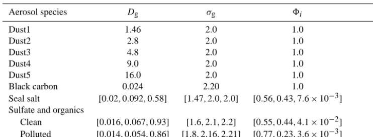
Table 1. Log-normal size distribution parameters used in this study (Lance et al., 2004).Dg(µm) andσgare the geometric mean diameter
and dispersion, respectively.8iis the particle number fraction in modei. The “polluted” size distribution parameters for sulfate and organics are used when the total aerosol mass exceeds 5.0 µg m−3.
Aerosol species Dg σg 8i Dust1 1.46 2.0 1.0 Dust2 2.8 2.0 1.0 Dust3 4.8 2.0 1.0 Dust4 9.0 2.0 1.0 Dust5 16.0 2.0 1.0 Black carbon 0.024 2.20 1.0
Seal salt [0.02,0.092,0.58] [1.47,2.0,2.0] [0.56,0.43,7.6×10−3]
Sulfate and organics
Clean [0.016,0.067,0.93] [1.6,2.1,2.2] [0.55,0.44,4.1×10−2]
Polluted [0.014,0.054,0.86] [1.8,2.16,2.21] [0.77,0.23,3.6×10−3]
species, respectively, andϕx(Si, T ,s¯p,x)is the number of
ac-tive nucleation sites per particle (Phillips et al., 2013, 2008). The summation in Eq. (11) is carried out over five log-normal modes for dust, and single log-log-normal modes for black carbon and organics (Table 1). Primary biological par-ticles are not predicted by GEOS-5 and are not considered in this work. However, on a global scale, their effect on ice cloud formation may be small (Hoose et al., 2010). Since dust and soot aerosol are typically irregular aggregates rather than spherical particles, sp¯,x was obtained from the mean
sphere-equivalent particle volume, assuming a bulk surface area density of 10 m2g−1for dust (Murray et al., 2011) and
50 m2g−1for soot (Popovitcheva et al., 2008).
The BN09 parameterization also allows the calculation of
Scrit for cirrus (Eq. 6, Sect. 2.3.1). According to BN09, the
ice saturation ratio at which most IN freeze in a polydisperse aerosol population, Shet, is given by (Barahona and Nenes,
2009b)
Shet=max
"
1+Si,max−Nhet
∂N
het ∂Si
−1
,1 #
. (12)
If no IN are present, then Shet approaches the saturation
threshold for homogeneous freezing, Shom (Barahona and
Nenes, 2009b). Shet andShom represent the minimum
satu-ration ratio required for cloud formation by heterogeneous and homogeneous freezing, respectively. They thus have the same meaning as the critical saturation ratio of Eq. (6).Scrit
is then calculated as
Scrit=fhetShet+(1−fhet)Shom, (13)
wherefhet=Nhet/(Nhom+Nhet)is the fraction of ice crystals
produced by heterogeneous ice nucleation.
The grid cell averaged nucleated ice crystal concentration,
Ni,nuc, is calculated by weightingNis,nucover the distribution
of updrafts within each grid cell (Sect. 2.3.4):
Ni,nuc= wmax
R
0
Nis,nuc(wsub)φ (w, σ¯ w2)dwsub wmax
R
0
φ (w, σ¯ 2 w)dwsub
, (14)
whereφ (w, σ¯ w2)is the normal distribution andwmax= ¯w+
4σw (Sect. 2.3.4). The latter is used as an upper limit to the integral to avoid numerical instability. Note that, for ice nu-cleation, using the approximation Ni,nuc≈Ni,nuc
w¯+
sub
may introduce a much larger bias than for cloud droplet activation (Sect. 2.3.2). This is because the competition between ho-mogeneous and heterogeneous nucleation introduces strong nonlinearity in Ni,nuc (Barahona and Nenes, 2009a). The
characteristic value ofwsubforNi,nuctherefore generally
dif-fers from the average vertical velocity. PDF averaging is also applied forScritandSi,max.
The contribution of ice nucleation in cirrus to the ice crys-tal number concentration is given by
dNi dt
cirrus,nuc
= (15)
max[Ni,nucPq(qt> Scritqi∗)−Ni, 0]
1t .
The factor Pq(qt> Scritqi∗)accounts for the probability of finding an air mass leading to cloud formation within the grid cell. This term was proposed by Barahona and Nenes (2011) to account for the effect of prior nucleation events on current cloud formation.
For the mixed-phase regime (T >235 K), Eq. (11) is ap-plied directly by assuming saturation with respect to liquid water, to find the contribution of deposition and condensa-tion heterogeneous nucleacondensa-tion to Ni. In this regime, cloud
treated as follows. The tendency inNifrom immersion freez-ing of cloud droplets is parameterized in the form
dN i dt imm =X x
Nxsp¯ ,xγc dns,x
dT exp(− ¯sp,xns,x), (16)
where γc= − ¯wsubddTz is the average cooling rate (Sect. 2.3.4). Nx and ns,x are the number concentration
and the active site surface density for species x, respectively. The latter is calculated according to Niemand et al. (2012) for dust and Murray et al. (2012) for black carbon.
Contact ice nucleation is parameterized as the product of the collection flux of aerosol particles by the cloud droplets and the ice nucleation efficiency in contact mode. Young (1974) suggested that phoretic effects and Brownian motion are responsible for collection scavenging of ice nu-clei. Baker (1991) however showed that Brownian motion is the dominant factor, although phoretic effects may be signifi-cant in deep convective clouds (Phillips et al., 2007). Consid-ering only Brownian collection, the contribution of contact ice nucleation to the ice crystal formation tendency is written in the form
dN i dt cont = (17) X x dNx dt Brw
1−exp[− ¯sp,xns,x(Tcont)] ,
where dNx dt
Brw is the Brownian collection flux of the
x aerosol species (Young, 1974). Consistent with laboratory studies (e.g., Fornea et al., 2009; Ladino et al., 2011), the active site density in the contact mode is assumed to be the same as for immersion freezing shifted towards a higher tem-perature; i.e.,Tcont≈T−3 K.
The in-cloud contribution of ice nucleation in mixed-phase clouds to the ice crystal number concentration tendency is given by
dN
i
dt
mixed,nuc
= (18) min " dNi dt cont + d Ni dt imm + d Ni dt dep ,Nd
1t
#
,
where the subscripts cont, imm, and dep refer to contact, im-mersion, and deposition/condensation ice nucleation, respec-tively. The term Nd
1t is used to limit the nucleated ice crystal concentration to the existing concentration of cloud droplets. 2.3.4 Subgrid-scale dynamics
Besides information on the aerosol composition and size, pa-rameterization of cloud droplet and ice crystal formation re-quires knowledge of the vertical velocity,wsub, on the spatial
scale of individual parcels (typically under 100 m), which is
not resolved by GEOS-5.wsubdepends on radiative cooling (Morrison et al., 2005), turbulence (Golaz et al., 2010), grav-ity wave dynamics (e.g., Barahona and Nenes, 2011; Kärcher and Ström, 2003; Jensen et al., 2010; Joos et al., 2008) and local convection. To account for these dependencies, we em-ploy a semi-empirical formulation as follows.
In situ measurements (e.g., Peng et al., 2005; Bacmeister et al., 1999; Conant et al., 2004) suggest thatwsubis
approx-imately normally distributed. The mean vertical velocity of the distribution is written as (Morrison et al., 2005)
¯
w=wls− cp g ∂T ∂t rad , (19)
wherewls is the grid-scale vertical velocity, cp is the heat capacity of air,gis the acceleration of gravity, and ∂T∂tradis the diabatic heating due to radiative transfer. Variance inwsub
for stratiform clouds results from subgrid-scale eddy motion,
σw,2turb, and gravity wave dynamics,σw,2gw; i.e.,
σw2=σw,2turb+σw,2gw. (20)
A first-order closure is used to diagnoseσw,2turb (Morrison and Gettelman, 2008):
σw,2turb=KT
lm , (21)
whereKT is the mixing coefficient for heat (Louis et al., 1983) andlmis the mixing length. MG08 prescribed a fixed
lm=300 m. To account for the spatial variation of lm, the formulation of Blackadar (1962) is used instead; i.e.,
lm= kz
1+ kz λm
, (22)
wherekis the von Kármán constant,zis the altitude andλm
is the value oflmin the free troposphere (Blackadar, 1962). The latter is estimated as 10 % of the boundary layer height from the previous time step (Molod, 2012). This approach also takes into account the vertical variation of lm within the planetary boundary layer (PBL). The minimum value of
σw,2turbis set to 0.01 m2s−2within the PBL.
Small-scale gravity waves strongly affect the formation of cirrus and mixed-phase clouds (e.g., Haag and Kärcher, 2004; Jensen et al., 2010; Joos et al., 2008; Barahona and Nenes, 2011; Dean et al., 2007). In situ measurements sug-gest that the dynamics of the upper troposphere are charac-terized by the random superposition of gravity waves from different sources (e.g., Jensen and Pfister, 2004; Bacmeister et al., 1999; Sato, 1990; Herzog and Vial, 2001). Random wave superposition results in a Gaussian distribution of ver-tical velocities (e.g., Bacmeister et al., 1999; Barahona and Nenes, 2011). Using this, a semi-empirical parameterization forσw,2gwis derived in the form (Eq. B5)
σw,2gw=0.0169min
"
4π U|τ0| ρaLcN
,
2π U2 N Lc
2#
whereτ0is the surface stress (Lindzen, 1981),Uthe horizon-tal wind,ρathe air density,N the Brunt–Väisälä frequency, andLcthe wavelength of the highest-frequency waves in the spectrum, also referred to as the characteristic cirrus scale (here assumed to be 100 m). Equation (23) is obtained by relating|τ0|to the equivalent perturbation height at the
sur-face. This is scaled to obtain the maximum wave amplitude at each vertical level (Joos et al., 2008; McFarlane, 1987) and then used to compute σw,2gw (Barahona and Nenes, 2011). This approach parameterizes orographically generated grav-ity waves. In practice, both the background and the oro-graphic surface stress are used in Eq. (23) to avoid underesti-mation ofσw,2gwin marine regions. The second term in brack-ets on the right-hand side of Eq. (23) limitsσw,gwto account
for wave saturation and breaking (Eq. B3). The derivation of Eq. (23) is detailed in Appendix B. Only activation pro-cesses are modified by subgrid vertical velocity variability; i.e.,φ (w, σ¯ w2)is assumed to be uncorrelated with the subgrid distribution of condensate.
2.3.5 Preexisting ice crystals
Ice nucleation can be inhibited by water vapor deposition onto preexisting ice crystals (i.e., ice crystals present in the grid cell from previous nucleation events). Their impact on cirrus properties may be significant at low temperatures, where ice crystals are small and have low sedimentation rates (Barahona and Nenes, 2011). The effect of preexisting crys-tals on ice nucleation can be parameterized by reducing the vertical velocity for ice nucleation in cirrus by a factor de-pendent on the preexisting ice crystal concentration and size (Eq. C5); i.e.,
wsub,pre= (24)
wsubmax
1−Ni,preπβcρiAi(Shom−1) 2λ0,i,preαwsubShom
,0
,
where Ni,pre is the preexisting ice crystal concentration, λ0,i,preis the slope of the size distribution of preexisting ice
crystals,cis a shape factor (here assumed to be equal to 1),
ρiis the bulk density of ice, andAi,αandβare temperature-dependent parameters (Appendix D). wsub,pre represents a
corrected vertical velocity accounting for the effect of pre-existing ice crystals limiting expansion cooling. Water vapor deposition onto preexisting crystals acts against the increase in ice supersaturation from expansion cooling. Thus, by en-hancing water vapor deposition within cloudy parcels, preex-isting ice crystals tend to decreaseSi,max(Eq. 10), leading to
a reduction inNi,nuc. To account for this,Si,maxis calculated
using wsub,preinstead ofwsub; i.e.,Si,max=Si,max(wsub,pre, T,Nhet). A similar approach was proposed by Kärcher et al.
(2006), who used a numerical integration technique instead of the analytical approach presented here. The derivation of Eq. (24) is detailed in Appendix C. The effect of preexisting ice crystals on cirrus properties is analyzed in Sect. 4.
2.4 Microphysics of convective cumulus
While all the main features of RAS are preserved in the new scheme, the removal of condensate is reformulated to ac-count for the effect of IN and CCN emissions on the genera-tion of convective precipitagenera-tion. RAS calculates the convec-tive cloud condensate and mass flux at each model level by averaging over an ensemble of ascending parcels, each one lifted from the top of the PBL (Molod et al., 2012; Rienecker et al., 2008). Each ascending parcel is characterized by its detrainment level and entrainment rate (Moorthi and Suarez, 1992), and saturation adjustment is used to find the amount of condensate present in each parcel. In the current RAS imple-mentation in GEOS-5, a single parcel detrains at each model level, so that the tendency of the tracerηdue to cloud con-vective processes is given by
∂η
∂t
cv
=Dη−gW∂η
∂p, (25)
whereDis the detrainment rate andW the convective mass flux. In the operational GEOS-5, a prescribed fraction of con-densate is assumed to precipitate from each parcel before reaching the cloud top. The remaining condensate is then linearly partitioned between ice and liquid as a function of
T and detrained at the neutral buoyancy level.
Each convective parcel is assumed to develop indepen-dently, and the detrained condensate from different parcels is weighted by the convective mass flux. The subscript “cp” in the following equations refers to processes occurring within each parcel. A detailed description of the GEOS-5 convective scheme is presented elsewhere (Moorthi and Suarez, 1992; Rienecker et al., 2008). The balance of a tracer,η, within a convective parcel is written as
1
W
d(ηW )
dt =
dη dt
cp
+λwcp(η0−η), (26)
whereddηt
cpis the rate of change inηfrom microphysical
processes occurring within convective parcels,wcpis the par-cel vertical velocity,λis the per-length entrainment rate, and
η0is the value of ηin the cloud-free environment. Detrain-ment of condensate is assumed to occur only at the cloud top.
The rate of change inηfrom microphysical processes oc-curring within a convective cloud parcel is given by
dη dt
cp
= dη
dt
source
+ dη
dt
precip
+ dη
dt
freezing , (27)
anvil; i.e.,hW1 d(ηW )dt i
cloud top
=Dη. The initial condition for Eq. (26) depends on the tracer. At cloud base, the concentra-tion of ice crystals and the ice mass mixing ratio are assumed to be zero, whereas the activation of cloud droplets at cloud base is explicitly considered (Sect. 2.4.2).
Solution of Eq. (26) requires knowledge of the vertical ve-locity within each parcel, wcp, which is also necessary for driving the droplet activation and ice nucleation parameter-izations. This is calculated by solving (Frank and Cohen, 1987)
1 2
dw2cp
dz = g
1+γ
Tv−Tv0 T0
v
−λw2cp−gqcn, (28)
where γ=0.5 (Sud and Walker, 1999), Tv and Tv0 are the virtual temperature of the cloud and the environment, re-spectively, andqcnis the mixing ratio of total condensate in the convective parcel. The first term on the right-hand side of Eq. (28) represents the increase in the convective par-cel’s kinetic energy by buoyancy, whereas the second and third terms account for the entrainment of stagnant air into the parcel and the drag from the weight of the condensate, respectively. Equation (28) is forward-integrated from the level below cloud base to cloud top usingwcp,in=0.8 m s−1
as an initial condition (Guo et al., 2008; Gregory, 2001); the vertical profilewcp is not very sensitive to this
assump-tion (Sud and Walker, 1999). Note that wcp,in differs from
the vertical velocity used for cloud droplet activation. The latter depends on the local buoyancy; i.e., wcp,cloudbase= wcp,in+
dwcp
dz 1zbase, where1zbase is the model layer thick-ness at the cloud base.
2.4.1 Partitioning of convective condensate
Total condensate is partitioned between liquid and ice as fol-lows. Nucleated ice crystals are assumed to grow by accre-tion of water vapor in an environment saturated with respect to liquid water. That is, the coexistence of liquid water favors a high concentration of water vapor available for deposition onto the ice crystals, and the ice and liquid phases remain in quasi-equilibrium within the convective parcel. Hydrometeor species are assumed to follow a gamma distribution (Eq. 2). The growth rate of ice crystals within convective cumulus is given by (Pruppacher and Klett, 1997; Korolev and Mazin, 2003)
d
qi
dt
dep
=min n
i,cpπ cρiAi(Si,wsat−1)
2λ0,i,cp
,dqcn
dt
, (29)
where dqcn dt
is the rate of generation of total condensate calculated by the convective parameterization,c is a shape factor (assumed equal to 1),ρithe bulk density of ice,Aiis a
temperature-dependent growth factor (Appendix D),ni,cpis
the ice crystal concentration within the convective parcel,λ0,i
is the slope parameter of the ice size distribution within the
convective parcel, andSi,wsatis the value ofSi at saturation
with respect to liquid water. Using Eq. (29), and sinceqcn=
ql+qi, the source term for liquid water within convective cumulus is given by
d
ql
dt
cond
= d
qcn
dt
−
d
qi
dt
dep
, (30)
where dql dt
cond is the rate of generation of liquid water
within convective parcels.
2.4.2 Droplet activation and ice crystal nucleation in convective cumulus
Explicit activation of CCN into cloud droplets is only con-sidered at cloud base and used as an initial condition to Eq. (26) (Sect. 2.4). Entrained aerosols (sulfate, sea salt, and organics) above cloud base are assumed to activate instan-taneously as they enter the cloud parcel. Dust and soot IN lead to the heterogeneous freezing of cloud droplets in the immersion and contact modes, described using Eqs. (16) and (17). Since soot and dust particles would likely adsorb water within convective parcels (Wiacek et al., 2010; Kumar et al., 2009a), ice nucleation in the deposition mode within convec-tive cumulus is not considered. Cloud droplets freeze homo-geneously at 235 K. Frozen droplets rapidly quench supersat-uration within convective cumulus. The homogeneous nucle-ation of deliquesced sulfate, which requires high supersatu-ration (Si∼145–170 %, Koop et al., 2000), is thus not likely
to occur within convective parcels. Homogeneous freezing of interstitial aerosol is therefore not considered within convec-tive cumulus.
2.4.3 Generation of convective precipitation
Precipitation is generated within each convective parcel and assumed to reach the surface during each time step. The re-maining condensate is then detrained into anvil clouds fol-lowing Eq. (25). Ice water in convective cumulus is likely to exist as graupel, snow and ice crystals with different size distributions and falling velocities, affecting the formation of precipitation. Following Del Genio et al. (2005), a simplified treatment is proposed, where total ice is partitioned between ice and snow (assumed as a single species) and graupel. The two species are differentiated by their terminal velocity. This partitioning is prescribed as a function of temperature and used to calculate the formation of ice precipitation within convective clouds. For ice crystal growth and detrainment a single ice species is assumed.
Total ice water within convective parcels is assumed to partition between ice/snow (taken as a a single species) and graupel, and differentiated by their terminal velocity (Ta-ble 2). The fraction of total ice existing as graupel is approx-imated by (Del Genio et al., 2005)
fgr=0.25{3.0+exp[0.1 min(T−273,0)]}. (31) The particle sizes of ice/snow and graupel are assumed to follow an exponential distribution (µg=µi/s=0.0)
(McFar-quhar and Heymsfield, 1997). The number precipitation rate of ice/snow within convective parcels is given by the number flux across the critical size for the ice/snow species,Dc,i/s
(Seinfeld and Pandis, 1998), dni
/s
dt
precip,cp
= (32)
ni/sAi(Si,wsat−1) Dc2,i/s
[1−exp(−λ0,i/sDc,i/s)],
where ni/s=(1−fgr)ni,cp is the number concentration of
ice/snow particles, and λ0,i/s is the slope parameter of the
ice/snow size distribution. The mass precipitation rate of ice/snow is calculated as
dqi /s
dt
precip,cp
=qi/sξi/s
ni/s
dni /s
dt
precip,cp
, (33)
where qi/s=(1−fgr)qi,cp is the mixing ratio of ice/snow
within the convective parcel, and ξi/s=16[(λ0,i/sDc,i/s)3+ 3(λ0,i/sDc,i/s)2+6λ0,i/sDc,i/s+6] is the ratio of the
vol-ume to number fraction aboveDc,i/s in the size distribution
of ice/snow. The term ξi/s is introduced to account for the
preferential precipitation of the largest particles of the pop-ulation, which tends to enhance the mass over the number precipitation rate. The critical size for precipitation, Dc,i/s,
is calculated by equating the hydrometeor terminal velocity,
wterm, towcp(Table 2).
Equations (32) and (33) assume that ice and snow grow mainly by diffusion within the convective parcel. The same assumption cannot be applied to graupel since it also grows by collection of cloud droplets. The precipitation rate of graupel is therefore calculated by removing the fraction of the size distribution above the graupel critical size,Dc,g, at
each model level (Ferrier, 1994) dngr
dt
precip,cp
=ngrexp(−λ0,gDc,g)
1tL
, (34)
where ngr=fgrni,cp is the graupel number mixing ratio, λ0,gthe slope parameter of the graupel size distribution and 1tL=1zw¯cv−1 is the time spent by the parcel in a given
model layer. Similarly forqgr, dqgr
dt
precip,cp
= (35)
qgrexp(−λ0,gDc,g)[(λ0,gDc,g)3+3(λ0,gDc,g)2+6λ0,gDc,g+6]
61tL
,
whereqgr=fgrqi,cpis the graupel mass mixing ratio.
The total mass precipitation rate for ice within convective parcels is given by
dqi dt
precip,cp
= dqi
/s
dt
precip,cp
+ dqgr
dt
precip,cp
. (36)
Similarly for the ice crystal number concentration, dn
i
dt
precip,cp
= dn
i/s
dt
precip,cp
+ dn
gr
dt
precip,cp . (37)
Equations (36) and (37) are used into Eq. (27), which then is used to solve Eqs. (25) and (26). Since graupel is not ex-plictly detrained, only the total ice (ice/snow plus graupel) is used in Eq. (27).
3 Model evaluation
Model evaluation is carried out by comparing cloud prop-erties against satellite retrievals and in situ observations. Satellite data sets included level 3 products from the NASA MODIS (http://modis.gsfc.nasa.gov/) combined TERRA and AQUA data product (Platnick et al., 2003), and the Interna-tional Satellite Cloud Climatology Project (ISCCP) (Rossow and Schiffer, 1999) and CloudSat (Li et al., 2012, 2014) projects. Level 3 MODIS monthly output for the years 2003– 2009 was used. CloudSat data spanned over the years 2007– 2008 and a climatology for the years 1983–2008 was used for ISCCP data (Rossow and Schiffer, 1999). When possi-ble, the Cloud Feedback Model Intercomparison Project Ob-servation Simulator Package, COSP (Bodas-Salcedo et al., 2011), was used to compare model output against satellite re-trievals. COSP uses the model output to simulate the retrieval of satellite platforms, minimizing in this way errors from the sampling of the model output when comparing against satel-lite observations.
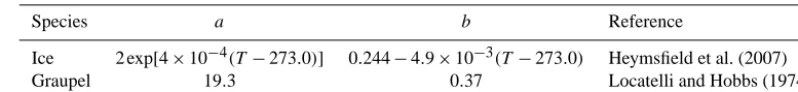
Table 2. Parameters of the terminal velocity relationwterm=aDyb(1000/p)0.4(SI units) for convective ice species.
Species a b Reference
Ice 2 exp[4×10⁻⁴(T−273.0)] 0.244−4.9×10⁻³(T−273.0) Heymsfield et al. (2007) Graupel 19.3 0.37 Locatelli and Hobbs (1974)
two years were enough to elucidate the first-order effect of variation in microphysical parameters on cloud properties. All simulations were forced with observed sea surface tem-peratures (Reynolds et al., 2002). Initial conditions were ob-tained from the Modern-Era Retrospective Analysis for Re-search and Applications (MERRA; Rienecker et al., 2011). The aerosol concentration was calculated interactively using the GOCART model (Colarco et al., 2010), with emissions as described in Diehl et al. (2012). Results obtained with the op-erational version of GEOS-5 and using the new microphysics are referred to as the CTL and NEW runs, respectively. 3.1 Cloud fraction
The parameterization of cloud fraction in GEOS-5 was mod-ified to account for the effect of microphysical processing on
Pq(q) (Sect. 2.3.1) and allow supersaturation with respect to the ice phase. Figure 1 shows the effect of these modifi-cations on the low (CLDLO), middle (CLDMD), and high (CLDHI) cloud fraction in GEOS-5. In general the CTL and NEW simulations present similar distributions of cloud frac-tion. However, in NEW, fc tends to be higher and in bet-ter agreement with ISCCP retrievals. The new cloud fraction scheme resulted in higher CLDLO in the remote Atlantic and Pacific oceans and reduced the cloud bias over South Amer-ica and Asia. CLDLO associated with the low-level stratocu-mulus decks on the western coasts of North and South Amer-ica and South AfrAmer-ica is still underpredicted in the NEW simu-lation. This feature is common in climate models (Kay et al., 2012); in GEOS-5 it is likely caused by the absence of an ex-plicit shallow cumulus parameterization. The overprediction of CLDLO at the high latitudes of the NH in CTL is also sig-nificantly reduced in the NEW simulation. Overall, the global mean bias in CLDLO is significantly lower in NEW (−3 %) than in CTL (−5 %).
The global mean bias in CLDMD is also lower in NEW (−9 %) than in CTL (−15 %). The overestimation of CLDMD at the low and middle latitudes of the South-ern Hemisphere (SH) and the NorthSouth-ern Hemisphere (NH) in CTL is largely removed in NEW, which results from a more realistic distribution of ice water content in NEW than in CTL (Sect. 3.6). The underestimation in CLDMD at the middle latitudes (∼30◦) of NH is also smaller in NEW than in CTL, particularly over land. However, NEW tends to increase the overestimation in CLDMD at the high lati-tudes of the SH. Similarly, although the CTL and the NEW simulations present similar distributions of high-level clouds
Figure 1. Annual mean differences in low- (CLDLO), middle-(CLDMD) and high- (CLDHI) level cloud fraction between GEOS-5 and ISCCP (Rossow and Schiffer, 1999) for the CTL and NEW runs using the COSP simulator.
(CLDHI), in general CLDHI tends to be overestimated at the marine high latitudes and underestimated over the continents. The NEW simulation also tends to underpredict CLDHI over the Tropical Warm Pool. The global mean bias in CLDHI is about 1 and 4 % in the CTL and NEW run respectively. Bi-ases in CLDHI and CLDMD at the high latitudes (above 60◦) of the SH and the NH tend to be more pronounced in NEW than in CTL. Although the source of these biases is not clear, they may be related to a low value ofq∗ (Eq. 4) in mixed phase clouds. Note that ISCCP retrievals tend to be uncertain in those regions as well (Rossow and Schiffer, 1999). 3.2 Supersaturation over ice
Restricting cloud formation toSi> Scrit implies that
super-saturation must be built before new ice clouds can form. The termPq(qt> Scritqi∗)in Eq. (15) also restricts ice nucleation
to supersaturated regions and reduces the nucleated ice crys-tal concentration and the water vapor relaxation time scale. Furthermore, MG08 allows for supersaturation within cirrus since it does not apply saturation adjustment for ice clouds. These factors lead to sustained supersaturation at cirrus lev-els (T <235 K).
Cloud formation and ice crystal nucleation are controlled in part byScrit, which provides an internal link between ice nucleation,fc andqi. Scrit depends on T and on the local
vertical velocity at the scale of individual cloudy parcels (∼100 m to 1 km).Scrit is also determined by the
availabil-ity of IN: in general, high IN concentration leads to lowScrit
(Barahona and Nenes, 2009b). The global distribution ofScrit
Figure 2. Annual zonal mean (left panel) and global frequency distribution (right panel) of the critical saturation ratio,Scrit(%),
for the cirrus regime (T <235 K), obtained from 6 h instantaneous GEOS-5 output over a 3-year subset (2002–2004) of the NEW run. Solid bold lines (left panel) represent the annual mean tropopause pressure.
120 %) and homogeneous (Scrit∼150 %) ice nucleation. The
peak at 150 % and the highest Scrit values correspond to
lowT regions with high vertical velocities and low aerosol concentration, common around the tropopause (Fig. 2, left panel). Values ofScrit as low as 105 % are also not
uncom-mon, and are associated with high concentrations of active IN (e.g., dust). These are often located aroundT ∼230–240 K, where deposition/condensation IN are active and abundant enough to impact supersaturation (Sect. 3.5). For lower T, the concentration of active IN is too low to decrease supersat-uration substantially, andScritincreases towardsShom(Fig. 2, left panel).
The global mean value ofScrit(∼144 %) is close toShom, which would in principle indicate a strong predominance of homogeneous nucleation (Fig. 2, left panel). This however depends on whether a cloud is actually formed under those conditions. Although high values of Scrit are very frequent
for p <50 hPa, most cirrus clouds form between 100 and 300 hPa (Sect. 3.6), whereScrit∼110–130 %. At these
ver-tical levels,Scritis relatively high (∼130 %) in the Southern
Hemisphere, but lower in the Northern Hemisphere. Homo-geneous freezing would thus tend to be more predominant in the Southern Hemisphere. This behavior is further analyzed in Sect. 3.5.
The distribution of clear sky saturation ratio,Si,c=(qv− fcq∗)/(1.0−fc), is shown in Fig. 3. In-cloudSiis assumed to be 100 %. In reality, supersaturation relaxation may be slow in cirrus clouds, particularly at low T (Krämer et al., 2009; Barahona and Nenes, 2011). However, it is expected that for
p >200 hPa most supersaturation is relaxed inside clouds over the time step of the simulation (∼1800 s) (Barahona and Nenes, 2008). Figure 3 also shows data from the AIRS (Atmospheric Infrared Sounder) (Gettelman et al., 2006) and MOZAIC (Measurement of ozone and water vapor by Airbus in-service aircraft) (Gierens et al., 1999) projects. The un-certainty in the retrieval increases with Si,c. However, both
MOZAIC and AIRS data show an exponential decrease in
Figure 3. Global frequency distribution of clear sky saturation ratio with respect to ice obtained from 6 h instantaneous GEOS-5 output over a 3-year subset (2002–2004) of the NEW run (left panel, black dots). Filled areas correspond to the frequency distributions from AIRS (solid area) satellite retrievals (Gettelman et al., 2006) and the MOZAIC (hatched area) data set (Gierens et al., 1999), respec-tively, for the years 2002–2004. Uncertainty in the observations was calculated as one standard deviation around the mean value within a 2◦×2◦grid cell and introducing a 10 % perturbation inSialong
thexaxis. The center and right panels show the zonal mean fre-quency (%) of clear sky supersaturation from GEOS-5 and AIRS, respectively.
P (Si,c)with increasingSi,c(Fig. 3, left panel). GEOS-5 also
shows this exponential decrease and is in agreement with AIRS and MOZAIC data. The peak P (Si,c)in the model is shifted towardsSi,c∼100 % since retrievals tend to avoid
zones withSi,c∼100 % near the cloud edges (Gettelman and
Kinnison, 2007). The frequency ofSi,c>101 % in GEOS-5
distributes almost symmetrically around the tropics (Fig. 3, middle panel), with a slightly higher probability of supersat-uration in SH than in NH. This is in part due to lower IN con-centrations in SH (Fig. 7), although differences in the dynam-ics of SH and NH also play a significant role. In agreement with AIRS data (Fig. 3, right panel), GEOS-5 predicts about 10 % supersaturation frequency in the upper tropical lev-els. GEOS-5 seems to slightly overpredictP (Si,c>100 %)
above 300 hpa at the high latitudes of the NH and SH and near the TTL; however, the uncertainty in the retrieval in these regions is also high (Gettelman and Kinnison, 2007). 3.3 Subgrid-scale vertical velocity
The nucleation of ice crystals and cloud droplets is strongly influenced by the subgrid-scale vertical velocity, wsub.
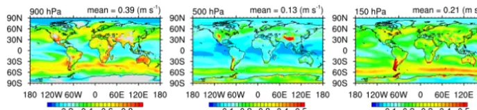
Figure 4. Annual mean subgrid vertical velocity standard deviation,σw, for the NEW run.
Figure 5. Annual vertically integrated droplet number concentration (106cm−2) from GEOS-5 using the Fountoukis and Nenes (2005) (FN05) and Abdul-Razzak and Ghan (2000) (ARG) CCN activation parameterization, and from the MODIS retrieval, calculated using Eq. (38). Data for latitudes higher than 60◦have been excluded from the analysis.
cloud base in marine stratocumulus (Peng et al., 2005; Guo et al., 2008), and continental regions (Fountoukis et al., 2007; Tonttila et al., 2011), showing σw mostly between 0.2 and 1 m s−1. However, global measurements ofσ
whave not been reported. Compared to similar schemes (e.g., Golaz et al., 2010) Eq. (21) results in higher velocities within the PBL since the characteristic length decreases near the surface, consistent with the vertical momentum balance within the PBL (Blackadar, 1962). σw2 thus rarely hits the prescribed minimum (∼0.01 m s−1) within the PBL.
Gravity wave motion dominates the global distribution of
σw at 500 and 150 hPa, being typically larger over land than over the ocean (Fig. 4). Air flowing over orographic fea-tures produces high-frequency waves that propagate to the free troposphere (Bacmeister et al., 1999; Herzog and Vial, 2001).σw is thus highest over the mountain ranges of Asia, South America, and the Antarctic. At 500 hPa,σw is about 0.1 m s−1 over land, and may reach up to 0.5 m s−1 over
mountain ranges. These values are in good agreement with in situ measurements (Gayet et al., 2004). A similar distribu-tion ofσwis found at 150 hPa, with values over land slightly higher than at 500 hPa. Over the ocean,σwis typically larger at 150 hPa than at 500 hPa, particularly over the tropics, since gravity waves in these regions can reach larger amplitudes before breaking. Figure 4 shows thatσwin the upper tropo-sphere varies by up to three orders of magnitude around the globe. Such variability has important implications for the ef-fects of IN emissions on cloud formation (Sect. 3.5). 3.4 Cloud droplet number concentration
Comparison of cloud droplet number concentration against satellite retrievals is typically challenging. Retrieval
algorithms generally introduce assumptions on the droplet size distribution that may bias the cloud droplet number concentration. To compare satellite retrievals and model data over the same basis, we take advantage of the output generated by the COSP MODIS simulator to obtain a “model retrieved” column-integrated droplet concentration, Nl,cum,
in the form (Han et al., 1998)
Nl,cum=
τ
2π R2eff,liq(1−b)(2−b), (38)
whereτ is the liquid cloud optical depth, b=0.193 (Han et al., 1998), and Reff,liq is the effective radius of cloud
droplets. To apply Eq. (38),Reff,liqandτ are obtained either
from the GEOS-5 COSP output or from the MODIS retrieval. This procedure does not aim to produce an accurate retrieval ofNl,cum, but rather to compare GEOS-5 and MODIS data
equally. Equation (38) is applied between 60◦S and 60◦N, where the MODIS retrieval is more reliable (Platnick et al., 2003).
Figure 5 shows the global distribution of Nl,cum from
GEOS-5 (NEW run, FN05) and MODIS. GEOS-5 is able to capture the highNl,cumfound in regions of high sulfate
emissions i.e., Europe, Central and Southeast Asia and the eastern coast of North America. There is also agreement be-tween MODIS and GEOS-5 in regions with high biomass burning emissions like Subsaharan Africa and South Amer-ica. However, the model tends to slightly underpredictNl,cum
in the remote Atlantic and Pacific Oceans. There is also underprediction ofNl,cumoff the western coasts of North and
South America and Africa. This is due to underprediction of shallow stratocumulus in GEOS-5 (Fig. 1) and becausewsub
Nl,cum in GEOS-5 (1.68 cm−2) is slightly lower than with
MODIS results (1.96 cm−2).
Droplet concentration is influenced by the CCN activation parameterization and the aerosol size distribution. The GO-CART model uses a single moment aerosol microphysics, and some uncertainty may result from assuming a fixed size distribution to obtain the aerosol number concentration. The impact of this assumption is discussed in Sect. 5. The sensi-tivity ofNl,cumto the CCN activation parameterization was
studied by implementing the Abdul-Razzak and Ghan (2000) activation parameterization (Fig. 5, middle plot) and is ana-lyzed in Sect. 4.
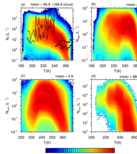
3.5 Ice crystal number concentration
At any givenT,Nivaries by up to four orders of magnitude, although mostly within a factor of 10 (Fig. 6a). The mean
Nipeaks around 200 L−1at 225 K, decreasing to∼20 L−1
at 190 K, and below ∼1 L−1 at 180 K. For T >245 K Ni
remains mostly below ∼10 L−1. Global meanNi is around
66 L−1 for all clouds and around 166 L−1 for cirrus (T <
235 K). Figure 6 shows agreement of GEOS-5 values with in situ measurements ofNi over the wholeT interval (Krämer
et al., 2009; Gultepe and Isaac, 1996). There is good agree-ment of GEOS-5 with field campaign data at T <200 K, where most models show a large positive bias (e.g., Barahona et al., 2010a; Salzmann et al., 2010; Gettelman et al., 2012). This results from the proper consideration of the effect of prior nucleation events on ice crystal nucleation (Section 2.3.3).Ni is also influenced by the presence of preexisting ice crystals; their effect is analyzed in Sect. 4.
The relative contribution of different mechanisms to the source of Ni is shown in Fig. 6. To facilitate comparison against in situ measurements, integrated variables, instead of number tendencies, are used. Thus, the ice crystal concen-tration from ice nucleation in the deposition and condensa-tion modes,Ndep, is calculated using Eq. (11) and the BN09
parameterization.Nifrom immersion freezing,Nimm, is
cal-culated by integration of Eq. (16) over the model time step. The concentration of detrained ice crystals,Ncnv, is given by
the ice crystal concentration at the cloud top calculated by Eq. (26).
Ndep varies mostly within the range from 0.1 to 50 L−1, and is largest around 240 K, where the aerosol concentra-tion is large enough to result in significant IN concentraconcentra-tion (Fig. 6b). There is however large variability inNdeparound the globe. Most deposition IN come from dust, although the concentration of black carbon IN may be significant, reach-ing 2 L−1 atT ∼230 K (not shown). A few deposition IN (∼1 L−1) are found atT as high as 260 K, mostly in regions of large dust concentration.
Nimm reaches up to 40 L−1 around 240 K, but decreases
rapidly for lower T, where it is prevented by the homoge-neous freezing of cloud droplets (Fig. 6c). In agreement with in situ observations of mixed-phase clouds (e.g., DeMott
Figure 6. Global frequency of in-cloud ice crystal number concen-tration as a function of temperature from 6 h instantaneous GEOS-5 output over a 3-year subset (2002–2004) of the NEW run. (a) Ice crystal concentration, Ni. Solid lines represent the 25 and 75 %
quantiles from the field campaign data analysis of Krämer et al. (2009). Solid-dotted lines represent the typical range of meanNi
found in mixed-phase clouds (Gultepe and Isaac, 1996). (b) Ice crystal concentration from deposition/condensation ice nucleation, Ndep. (c) Ice crystal concentration from immersion ice nucleation, Nimm. (d) Ice crystal concentration from convective cumulus
de-trainment,Ncnv.
et al., 2010), immersion freezing IN are scarce above 250 K, with typical concentrations below 0.1 L−1. Dust is the most important source of immersion IN, whereas black carbon IN typically contribute less than 2 L−1toNi. Contact freezing
IN are not explicitly shown in Fig. 6, but they follow a sim-ilar tendency as immersion freezing IN, although with lower concentrations.
Ncnv remains below 50 L−1 for T >240 K, characteris-tic of heterogeneous ice nucleation. For T >250 K, Ncnv
reaches up to 10 L−1 mostly from immersion and contact freezing of supercooled droplets within the convective cumu-lus (Fig. 6d). Homogeneous freezing of cloud droplets is evi-dent in the strong increase inNcnvaroundT ∼240 K, which in some instances may reach up to 10 cm−3. Such very high
Nncv is responsible for the highest values of Ni in Fig. 6.
Along with immersion freezing, detrainment from convec-tive cumulus determinesNiforT >240 K.
Figure 7. Annual mean ice crystal concentration nucleated in cirrus (T <235 K) weighted by cloud fraction for the NEW run (left panel). Also shown are the weighted average (center panel) and zonal mean (right panel) fractions of ice crystal production by homogeneous freezing in cirrus.
Figure 8. Zonal mean non-convective ice water mass mixing ratio (mg kg−1) (upper panels) and total ice condensate (ice and snow, bottom panels) for non-convective clouds from the CTL and NEW runs and the CloudSat retrieval (Li et al., 2012). Model results span over 10 years of simulation, whereas CloudSat retrievals are plotted for the period 2007 to 2008.
weighted by cloud fraction) and zonal mean of the contri-bution of heterogeneous ice nucleation toNi,nuc are shown
in the middle and right panels of Fig. 7, respectively. Glob-ally, about 70 % of the production of ice crystals in cirrus proceeds by homogeneous freezing, with a clear contrast between the Northern Hemisphere (NH) and the Southern Hemisphere (SH). Homogeneous freezing is most prevalent in the SH, and only on the western coasts of South America and Africa is the contribution of heterogeneous freezing sig-nificant (∼30 %; Fig. 7, middle panel). By contrast, most of the NH is influenced by IN emissions, which in some cases dominate the ice crystal production.
Part of the higher predominance of heterogeneous ice nu-cleation in NH than SH is explained by the greater abundance of dust in NH. However, comparison of Figs. 4 (right planel) and 7 (left panel) also reveals a marked effect ofσw onNi.
Low σw tends to enhance the effect of IN on Ni because
of the greater residence time of the heterogeneously frozen ice crystals in the parcel before the onset of homogeneous freezing, and the lower rate of increase of supersaturation
Figure 9. Zonal mean non-convective liquid water mass mixing ra-tio (mg kg−1) (upper panels) and total liquid condensate (water and rain, bottom panels) for non-convective clouds from the CTL and NEW runs and the CloudSat retrieval (Li et al., 2014). Model re-sults span over 10 years of simulation, whereas CloudSat retrievals are plotted for the period 2007 to 2008.
(Barahona and Nenes, 2009a). Heterogeneous freezing thus tends to dominate ice crystal production in regions of lowσw and lowNi,nuc like Sub-Saharan Africa, the Arctic, and the
3.6 Cloud liquid and ice water
The implementation of the new microphysics resulted in sig-nificant improvement of the representation of ice and liquid water content in GEOS-5. Figure 8 shows the zonal mean ice mass mixing ratio,qi, from the NEW and CTL
simula-tion compared to the CloudSat retrieval for non-convective, non-precipitating ice (Li et al., 2012). The global distribution ofqiin the NEW simulation is in better agreement with the
satellite retrieval than that obtained in CTL. The excessive freezing around T =240 K, characterized by the bulls-eye pattern around 600 hPa in the CTL run, is not present in the NEW simulation. In absolute terms,qiin the NEW and CTL runs is generally lower than CloudSat data, although mostly within the intrinsic error of the retrieval, about a factor of 2 (Li et al., 2012; Eliasson et al., 2011). Including snow in the comparison (Fig. 8, bottom panels) still results in lower ice and snow concentration than in CloudSat, although within the error of the retrieval.
Figure 9 shows the zonal mean liquid mass mixing ra-tio, ql, from GEOS-5 for the CTL and NEW runs
com-pared against the CloudSat retrieval for convective, non-precipitating liquid water (Li et al., 2014). There is far lower
ql in the NEW than in the CTL run, particularly over the
tropics and the subtropics of the NH. Above 900 hPa, the spa-tial distribution ofql in the NEW run is in better agreement than CTL. In absolute termsql in NEW is closer to Cloud-Sat than in CTL. However, this must be taken with caution as CloudSat may not retrieve liquid water close to the ground (Devasthale and Thomas, 2012). The NEW and CTL simula-tions however show that most liquid water is held below the 850 hPa level in GEOS-5. The bottom panels of Fig. 9 also suggest that the rain mass mixing ratio is lower in NEW than in the CTL simulation and CloudSat. Still, the spatial distri-bution of the concentration of liquid and rain from NEW and from the CloudSat retrieval shows similar characteristics.
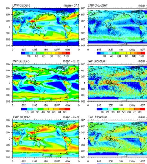
The spatial distribution of the liquid water path (LWP) (Fig. 10) in the NEW simulation is similar to that observed by CloudSat, although in general LWP is larger in the NEW simulation that in CloudSat, particularly over marine regions. Comparison against other retrievals reveals uncertainty in ex-perimental observations of LWP. Annual average LWP from MODIS is 144 g m−2, about twice as much as the GEOS-5 output when using COSP to simulate the MODIS retrieval (60 g m−2). MODIS however tends to predict higher LWP in polar regions than in the tropics, pointing to an artifact of the retrieval (Platnick et al., 2003). SSMI data (Spencer et al., 1989) is also typically used for model evaluation, although it is restricted to oceanic regions. Annual mean LWP from SSMI is about 84 g m−2, which is higher than predicted by GEOS-5 over the ocean (∼48 g m−2, not shown).
Figure 10 shows the annual mean IWP (non-precipitating, non-convective) from GEOS-5 and CloudSat (Li et al., 2012). In general there is reasonable agreement in IWP between CloudSat and GEOS-5, with and slightly higher
Figure 10. Liquid (LWP), ice (IWP), and total (TWP) water paths (g m−2) for non-convective, non-precipitating clouds from GEOS-5 output using the new microphysics and from the CloudSat retrieval (Li et al., 2012, 2014).
IWP in GEOS-5 (27.1 g m−2, NEW run) than in Cloud-Sat (25.8 g m−2). There is also uncertainty in IWP obtained
by different retrievals; however, a recent intercomparison showed agreement between the ISCCP and CloudSat re-trieved IWP (Eliasson et al., 2011). GEOS-5 is able to cap-ture the high IWP observed in the Tropical Warm Pool, Cen-tral Asia, and over the mountain ranges of Africa, and North and South America. The high IWP of the latter regions re-sults in part from strong ice crystal production over mountain ranges (Sect. 3.5). GEOS-5 however underestimates IWP in the tropical western Pacific Ocean. The spatial distribution of the total-water path (liquid and ice) is similar to that obtained with CloudSat, although the global mean TWP is higher in GEOS-5 (∼64 g m−2) than in the retrieval (∼49 g m−2) due to the larger LWP in GEOS-5.
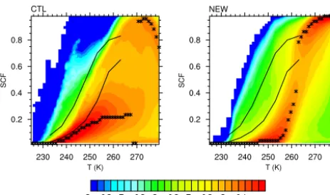
3.7 Supercooled cloud fraction