R E S E A R C H
Open Access
Proteobacteria explain significant
functional variability in the human gut
microbiome
Patrick H. Bradley
1and Katherine S. Pollard
1,2*Abstract
Background: While human gut microbiomes vary significantly in taxonomic composition, biological pathway abundance is surprisingly invariable across hosts. We hypothesized that healthy microbiomes appear functionally redundant due to factors that obscure differences in gene abundance between individuals.
Results: To account for these biases, we developed a powerful test of gene variability called CCoDA, which is applicable to shotgun metagenomes from any environment and can integrate data from multiple studies. Our analysis of healthy human fecal metagenomes from three separate cohorts revealed thousands of genes whose abundance differs significantly and consistently between people, including glycolytic enzymes, lipopolysaccharide biosynthetic genes, and secretion systems. Even housekeeping pathways contain a mix of variable and invariable genes, though most highly conserved genes are significantly invariable. Variable genes tend to be associated with Proteobacteria, as opposed to taxa used to define enterotypes or the dominant phyla Bacteroidetes and Firmicutes.
Conclusions: These results establish limits on functional redundancy and predict specific genes and taxa that may explain physiological differences between gut microbiomes.
Keywords: Human gut microbiome, Proteobacteria, Bacteroidetes, Firmicutes, Variance, Shotgun metagenomics, Statistical methods, Functional redundancy, Enterotypes, Human gut microbiome
Background
The microbes that inhabit the mammalian gut encode a wealth of proteins that contribute to a broad range of biological functions, from modulating the immune sys-tem [1–3] to participating in metabolism [4, 5]. Shotgun metagenomics is revolutionizing our ability to identify protein-coding genes from these microbes and associate gene levels with disease [6], drug efficacy [7] or side-effects [8], and other host traits. For instance, human gut microbiota associated with a traditional high-fiber agrar-ian diet encoded gene families involved in cellulose and xylan hydrolysis, which were absent in age-matched con-trols eating a typical Western diet [9]. The functional capabilities of the human gut microbiome go beyond sta-tistical associations. A number of microbial genes have
*Correspondence: [email protected] 1Gladstone Institutes, San Francisco, CA, USA
2Division of Biostatistics, Institute for Human Genetics, and Institute for Computational Health Sciences, University of California, San Francisco, CA, USA
now been causally linked to host physiology. Examples include the colitis-inducing cytolethal distending toxins of Helicobacter hepaticus[10] and the enzymes of commen-sal bacteria that protect against these toxins by producing anti-inflammatory polysaccharide A [11].
It is therefore surprising that healthy human gut micro-biomes have been characterized as functionally stable, with largely redundant gene repertoires in different hosts. We refer to these metagenomic gene families with very low variance in abundance across hosts as “invariable.” Several lines of evidence support this conclusion. First, biological pathway abundance tends to be less variable across metagenomes than it is between isolate genomes [12], suggesting strong selection for microbes that encode functions necessary for adaptation to the gut environ-ment. Second, the relative abundances of pathways are strikingly invariable compared to the relative abundances of bacterial phyla in the same metagenomes [12, 13]. Thus, it appears that humans harbor phylogenetically distinct
gut communities that all do more or less the same things, except in the context of disease or other extreme host phenotypes.
Functional redundancy deserves a closer look, however, because physiologically meaningful differences in gene abundances between healthy human microbiomes could easily have been missed. One primary factor may be that prior work did not look at quantitative abundances of indi-vidual genes but instead mainly summarized function at the level of Clusters of Orthologous Groups (COG) cat-egories (e.g., “carbohydrate metabolism and transport”) and KEGG modules (e.g., “citrate cycle”) [12–14]. This strategy lacks the power to detect one component of a pathway or protein complex that varies in abundance across hosts if other components are less variable. This masking of variable genes (i.e., genes with high variance) is likely because the presence and abundance of most COG categories and KEGG modules will be dominated by core components (i.e., housekeeping genes) that are widely distributed across the tree of life and abundant in metagenomes. The only previous analyses of individ-ual genes asked whether they were universally detected across all individuals sampled [12, 14]. However, uni-versally detected genes may still vary substantially in abundance, and conversely, lower-abundance invariable genes may not be universally detected merely due to sam-pling. This approach is also sensitive to read depth [12] and sample size [14]. Based on these observations, we were motivated to quantitatively investigate functional redundancy at the level of individual sets of orthologs (or “gene families”).
To enable high-resolution, quantitative analysis of func-tional stability in the microbiome, we developed a sta-tistical test that identifies individual gene families whose abundances are either significantly variable or invari-able across samples. We named this test CCoDA, for Covariate-Corrected Dispersion Analysis. The inputs to the method are gene abundance values (e.g., normalized counts of metagenomic reads mapping to a particular gene), and the outputs are lists of genes whose abundances differ significantly more or less than expected across sam-ples, which can be summarized by pathways and by the taxonomic groups contributing reads.
The study of variability, in addition to the more com-mon study of average abundances, is becoming more popular in other areas of genomics, such as gene expres-sion across tissues [15], epigenetic variation [16], and, especially, individual cells [17–21]. However, there are still few existing statistical approaches for determining whether a given observed amount of biological variabil-ity exceeds or falls beneath expectations, and the existing methods require the use of spike-ins to decompose tech-nical and biological variability [19, 20]. Our method does not require these additional data, which are often not
available in existing studies of the microbiome. Addi-tionally, it incorporates solutions to three major chal-lenges to studying functional redundancy with shotgun metagenomics data.
The first key innovation of our approach is using a test statistic that captures residual variability after accounting for the overall gene abundance. Like modern approaches for RNAseq analysis [22, 23] and proteomics analysis [24], we use the negative binomial distribution to directly model the sequencing count data and account for the mean-variance relationship. However, instead of using this distribution to more accurately detect genes with differences in abundance between groups, we use it to dis-cover genes whose variances are unexpected given their mean values. This modeling choice is important because abundant genes will be variable just by chance due to the correlation between mean and variance in any sequencing experiment. Conversely, phylogenetically restricted genes will have relatively low variance due to being less abun-dant. Furthermore, gene abundances can be sparse (i.e., zero in many samples). For all of these reasons, simply ranking genes based on their variances would yield many false positives and false negatives.
A second benefit of our modeling approach is that we can adjust for systematic differences in a gene’s mea-sured level between studies to allow for quantitative integration of data from multiple sources. Meta-analysis is essential for gaining sufficient power to detect vari-able genes across the range of mean abundance levels. It also ensures robustness and generalizability of discov-ered inter-individual differences, which occur by chance in small sets of metagenomes. Our modeling approach is also flexible enough to account for factors such as aver-age genome size that can affect measurements of gene abundances.
Finally, our method does not require predefined cases and controls but instead enables discovery of genes that explain functional differences between microbiomes with-out prior knowledge of which groups of samples to com-pare. This is critical for the current phase of microbiome research, when many factors influencing microbial com-munity composition are unknown. Gene families that contribute to survival in one particular type of healthy gut environment should emerge as variable between hosts and their functions may point to factors influencing com-munity composition, mechanisms of microbe-host inter-actions, and biomarkers of presymptomic disease (e.g., pre-diabetes).
across gut microbiota (e.g., central carbon metabolism and secretion), included significantly variable gene fami-lies. Phylogenetic distribution (PD) correlated overall with variability in gene family abundance, and exceptions to this trend highlight functions that may be involved in adaptation, such as two-component signaling and special-ized secretion systems. This approach to discovering func-tions that distinguish microbial communities is applicable to any body site or environment.
Finally, the human gut is normally dominated by the bacterial phyla Bacteroidetes and Firmicutes [13]. Clades within these phyla (especially Bacteroides, Prevotella, andRuminococcaceae) are the most commonly used to cluster individuals together into “enterotypes” [25–28] because they explain the most taxonomic variation. The Bacteroidetes-to-Firmicutes ratio has also been measured as a potential biomarker of interest in its own right [29–31]. In contrast, we show that the less abundant phy-lum Proteobacteria, and not Bacteroidetes or Firmicutes, is a major source of genes with the greatest variabil-ity in abundance across hosts. Thus, while Bacteroidetes and Firmicutes may contribute most to taxonomic varia-tion between hosts, the abundance of Proteobacteria may capture more of the functional variation. This has implica-tions for the interpretation of taxonomic data from human gut microbiota and, because of the link between Pro-teobacteria and dysbiosis [32], also suggests a potential relationship between inflammation and gene-level differ-ences in gut microbial functions.
Results
To describe variation within healthy gut microbiota across different human populations, we randomly selected 123 metagenomes of healthy individuals from the Human Microbiome Project (HMP, n = 42) [13], controls in a study of type II diabetes (T2D,n= 44) [33], and controls in a study of glucose control (GC, n = 37) [34]. These span American, Chinese, and European populations, respectively (see the “Methods” section). We mapped these metagenomes to KEGG Orthology (KO) families with ShotMAP [35] and counted reads for 17,417 gene families.
Accurately normalizing gene read counts so that they are comparable across samples and studies is critical to our meta-analytical approach and any quantitative eval-uation of shotgun metagenomes. We therefore quanti-fied gene family abundance using reads per kilobase of genome equivalents (RPKG) [36]. This method of calcu-lating abundances takes into account differences in the average genome size within different metagenomes, as well as factors such as gene length, that can also bias counts (long genes will generally have a greater proportion of reads).
Unadjusted calculation of gene variability yields misleading results
One straight-forward approach to determining gene fam-ily variability, which has previously been employed in the literature [13], would simply be to calculate the variance of gene family abundances across all datasets. The tails of this distribution—for example, the top and bottom 10%— could then be termed “variable” and “invariable” gene families. However, by this metric, the most “variable” gene families would actually be enriched for pathways such as the ribosome (FDR-correctedpvalueq = 2.4×10⁻¹⁰), DNA replication (q=0.07), and aminoacyl-transfer RNA (tRNA) biosynthesis (q=1.2×10⁻⁶). These results con-tradict biological intuition: it would be very surprising for genes within the best-conserved “housekeeping” path-ways to be among the most variable, since they appear in most microbial genomes. (Here, we define “house-keeping” gene families as those involved in fundamental, highly conserved cellular processes such as translation, DNA replication, and central metabolism). Indeed, out of a recent list of 74 protein-coding genes that were uni-versally present and single-copy in bacterial genomes, 14 were ribosomal genes and 10 were tRNA synthetases or tRNA modification enzymes [37]; “housekeeping” path-ways also dominated previous lists of bacterial universal and single-copy genes [38].
Furthermore, according to this same straight-forward metric, the least variable gene families would include those involved in disease signatures such as “salmonella infection” (q = 0.027), “pertussis” (q = 1.4×10⁻³), and
“legionellosis” (q=4.9×10⁻³). The presence of genes in
these disease signatures does not necessarily indicate the presence of that disease or an active infection. However, it seems unlikely for genes involved in pathogenicity to be among the most stable components of the healthy human microbiome.
The explanation for this counterintuitive result can be visualized by plotting the mean vs. variance for each mea-sured gene family (Fig. 1): in shotgun metagenomic data, mean and variance are tightly correlated over the entire range of means. This phenomenon is robust to the num-ber of samples assessed (Additional file 1: Figure S1). Similar mean-variance relationships are actually observed in other high-throughput sequencing applications, such as RNAseq [39, 40] (which is why standard hypothesis tests based on assuming normality are inappropriate for RNAseq data, if the correct variance-stabilizing transfor-mations are not applied [40]).
Fig. 1Shotgun metagenomic data show a very strong mean-variance relationship. The log10(mean) is plotted against log10(variance) for each gene family (points) in each study (headings). Bacterial ribosomal proteins (green), aminoacyl-tRNA charging genes (orange), and genes annotated to the T3SS-dependentSalmonellapathogenesis signature in KEGG (blue) are highlighted.Trend linesshow a Poisson (dashed blue line) and a negative binomial (dashed red line) fit to the count data. Negative binomial provides a better fit in all three data sets
will appear to be invariable when in reality they are sim-ply very infrequently observed. For example, three out of five of the invariable gene families annotated to pertussis only have one read each in a single sample, which con-stitutes extremely weak evidence for their presence in the metagenome, let alone invariability. This approach also leaves us unable to detect gene families that are variable but relatively abundant, as well as the opposite (Fig. 2a–d). Gene family abundances can also vary by study, because of both biological differences between populations and technical factors including library preparation, amplifica-tion protocol, and sequencing technology. However, gene families with large study effects may or not be variable within each study, and vice versa (see, e.g., Fig. 2e–h). Our method should therefore also take this potential con-founder into account.
Finally, to assess statistical significance, we need to assess the range of variances we would expect for a partic-ular gene family given its mean abundance, requiring us to model the overall mean-variance relationship. Figure 1 shows that this mean-variance relationship cannot be ade-quately captured by a Poisson distribution (blue dashed line), in which the mean and variance are equal; however, a better fit can be obtained by using the negative binomial distribution (red dashed line), a count-based distribution that allows for overdispersion, i.e., variance that exceeds
the mean. Indeed, simply based on this negative binomial best-fit, ribosomal proteins are likely less variable than expected since they fall well below the trend line in all three datasets (Fig. 1). The negative binomial is commonly used in other sequencing applications, such as RNAseq [21], which has similar overdispersion.
A new test, CCoDA, captures the variability of microbial gene families
We present a model that enables gene family abundance to be quantitatively compared across metagenomes for thou-sands of microbial genes. To account for study effects, we fit a linear model of log abundanceDg,sfor genegin sam-plesas a function of the overall mean abundanceμgand a termβg,ythat quantifies the offset for each studyy:
Dg,s=μg+
y∈Y
Iy,sβg,y+g,s (1)
where Iy,s is an indicator variable that is 1 if sample s belongs to studyyand 0 otherwise. In this simple model, βg,yis simply the mean of genegin studyyafter subtract-ing the overall meanμg, andg,sare the residuals left after these study-specific meansβg,yare subtracted out.
A
B
C
D
E
F
G
H
Fig. 2The residual variance statistic captures variation in gene families after accounting for between-study variation. Theleft-hand panels(“original abundances") showfilled circlesrepresenting log-RPKG abundances for gene families from the KEGG Orthology (KO), with per-study means shown in solid horizontal linesand the distance from these means shown asdashed vertical lines. Theright-hand panels(“residuals") show the same gene families after fitting a linear model that accounts for these per-study means, with an accompanying density plot showing the distribution of these residuals.Vgvalues in bold underneath density plots are the calculated variances of these residuals. These gene families are sets of orthologs corresponding to the genesatatA,bdevR,cwaaW,dthrC,egspA,ftssB,gdctS, andhecnB. Panelsa,bshow two invariable gene families with relatively high (a) and low (b) average abundance; similarly, panelsc,dshow two variable gene families with relatively low (c) and high (d) average abundances. Panelse,fshow two gene families involved in secretion with similar abundances, but low (e) vs. high (f) variability. Finally, panels
g,hshow that both invariable (g) and variable (h) gene families can have substantial study-specific effects. (All gene families displayed were significantly (in)variable using CCoDA, FDR≤5%)
across samples in the same study as s. We denote the variance of the residuals across samples by Vg. When this statistic is small, the gene has similar abundance across samples after accounting for study effects. A large value of Vg indicates that samples have very different abundances.
To assess the statistical significance of gene family ability, as suggested above, we compare the residual vari-anceVg to a data-driven null distribution based on the negative binomial distribution (see the “Methods” section and Additional file 2: Figure S2). This approach is nec-essary because there is no straight-forward formula for thepvalue ofVg. Our method looks for deviations from the null hypothesis that gene families in the dataset have the same mean-variance relationship. This relationship is
captured by the overdispersion parametersky, such that the variance for a genegin a studyyis given by:
σ2
g,y=βg,y+
β2
g,y ky
(2)
We validated this approach further and assessed type I and type II error rates with simulated data (see the “Methods” section, Additional file 4: Figure S4), find-ing that CCoDA has high power and good control over the false positive rate when the overdispersion param-eter k used in the null distribution is accurately esti-mated. To make the test more robust to factors affecting the estimation of k (Additional file 5: Figure S5), we also used simulation to control the false discovery rate empirically (Table 1).
CCoDA can be applied to shotgun metagenomes to sen-sitively and specifically identify variable genes in any envi-ronment without prior knowledge of factors that stratify relatively high versus low abundance samples.
Thousands of variable gene families in the gut microbiome Using CCoDA, we found 2357 gene families with more variability than expected and 5432 with less (leaving 9628 non-significant) at an empirical FDR of 5% (Additional file 3: Figure S6A). Restricting the analysis to gene families with at least one annotated representative from a bacterial or archaeal genome in KEGG, we obtained 1219 sig-nificantly variable and 3813 sigsig-nificantly invariable gene families (and 2194 non-significant). The differences in the residual variation of these gene families can be visual-ized using a heatmap of the residualg,svalues (Additional file 6: Figure S7 and Additional file 7: Figure S8). The large number of genes that were less variable than expected given their means supports the hypothesis of some func-tional redundancy in the gut microbiome, potentially due to selection for core functions that make microbes more successful in the gut environment. Notably, the HMP cohort tended to have overall lower variance in their metagenomes than the GC and T2D cohorts; this may be because the exclusion criteria for HMP, which explic-itly studied only healthy individuals, were particularly stringent [41]. Nevertheless, our discovery of thousands of significantly variable genes across a range of abun-dance levels demonstrates that the gut microbiome is less invariable than prior work suggested.
This result highlights the importance of a quantitative, gene-level evaluation of functional stability. Importantly, the magnitude of the residual variance statisticVgis not the sole determinant of significance, as illustrated by the
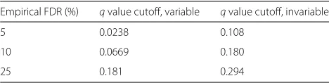
Table 1qvalue cutoffs to reach a given empirical FDR, estimated from simulation
Empirical FDR (%) qvalue cutoff, variable qvalue cutoff, invariable
5 0.0238 0.108
10 0.0669 0.180
25 0.181 0.294
overlap in distributions ofVgbetween the variable, invari-able, and non-significant gene families. For example, both low-abundance gene families with many zero values and high-abundance but invariable gene families will tend to have low residual variance, but the evidence for invari-ability is much stronger for the second group. Our test accurately discriminates between these scenarios, tending to call the second group significantly invariable and not the first (Additional file 3: Figure S6A, inset), whereas an approach that simply thresholdedVgwould be unable to distinguish between them.
Biological pathways contain both invariable and variable components
To test our hypothesis that the appearance of pathways and functional categories with similar abundance across samples can be explained by a subset of core compo-nents, we examined individual gene variability within KEGG modules. As expected, we observed an overall signal of stability at this broad level of gene groupings. Many of the pathways previously identified as invari-able (e.g., aminoacyl-tRNA metabolism, central carbon metabolism) indeed have more invariable than variable genes. However, individual genes show a much more complex picture. Even the most invariable pathways also include significantly variable genes (Fig. 3). For exam-ple, the highly conserved KEGG module set “aminoacyl-tRNA biosynthesis, prokaryotes” included one variable gene at an empirical FDR of 5%, sepRS. sepRS is an O-phosphoseryl-tRNA synthetase, which is an alternative route to biosynthesis of cysteinyl-tRNA in methanogenic archaea [42]. Methanogen abundance has previously been noted to be variable between individual human guts: while DNA extraction for archaea may be less reliable than for bacteria, even optimized methods showed large standard deviations across individuals [43]. Another gene in this category was variable at a weaker level of significance (10% empirical FDR): poxA, a variant lysyl-tRNA synthetase. Recent experimental work has shown that this protein has a diverged, novel functionality, lysinylating the elongation factor EF-P [44, 45].
By comparison, 77% of the tested prokaryotic gene families in the KEGG module set “central carbohy-drate metabolism” were significantly invariable, and 5.6% (five genes) were significantly variable (Additional file 8: Figure S9) at an empirical FDR of 5%. In this case, the vari-able gene families highlight the complexities of microbial carbon utilization (see Additional file 9 for details).
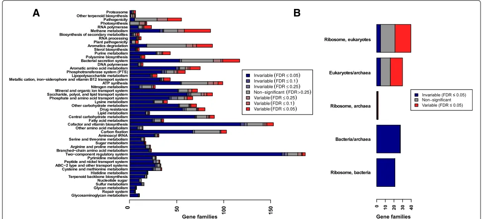
A B
Fig. 3Most pathways include a mixture of both variable and invariable gene families.aStacked bar plots show the fraction of invariable (blue), non-significant (gray), and variable (red) gene families annotated to KEGG Orthology pathway sets (rows), at different false discovery rate (FDR) cutoffs (color intensity). Only gene families with at least one annotated bacterial or archaeal homolog were counted.bFraction of strongly invariable, non-significant, and strongly variable gene families within the ribosomes of different kingdoms. Row labels with only one kingdom indicate gene families unique to that kingdom, and rows with multiple kingdoms (e.g., “Eukaryotes/archaea”) indicate gene families shared between these two kingdoms. As expected, the bacterial ribosome was completely invariable
Gram-negative bacteria and are often involved in spe-cialized cell-to-cell interactions, between microbes and between pathogens or symbionts and the host. They allow the injection of effector proteins, including virulence fac-tors, directly into target cells [46, 47]. Type VI secretion systems are also determinants of antagonistic interactions between bacteria in the gut microbiome [48, 49].
In contrast, gene families in the Sec (general secre-tion) and Tat (twin-arginine translocasecre-tion) pathways were nearly all significantlyinvariableat an empirical FDR of 5%, with only one gene in each being found to be sig-nificantly variable. This contradicts previous suggestions that the Sec and Tat pathways were some of the most variable in the human microbiome [13]. This discrepancy is probably due to our accounting for the mean-variance relationship in shotgun data. The Sec and Tat sys-tems are abundant and phylogenetically diverse [50] and will therefore have greater variance than low-abundance genes just by chance. Our test adjusts for this feature of sequencing experiments and shows that these genes are in fact less variable than expected given their mean abundance.
Our results further demonstrate that analyzing func-tional variability at the level of pathways can obscure gene-family-resolution trends of potential biomedical importance. The variability of individual gene families involved in lipopolysaccharide (LPS) metabolism may exemplify such a case. LPS (also known as “endotoxin”) is a macromolecular component of the Gram-negative
bacterial outer membrane, consisting of a lipid anchor called “lipid A,” a “core oligosaccharide” moiety, and a polysaccharide known as the “O-antigen” (which may be absent). Lipid A is sensed directly by the human innate immune system via the Toll-like receptor TLR4. Furthermore, lipid A variants with different covalent modifications (e.g., differentially acylated [51], phos-phorylated [52], and palmitoylated [53] variants) have been shown to have different immunological properties (see Additional file 9: Supplementary information).
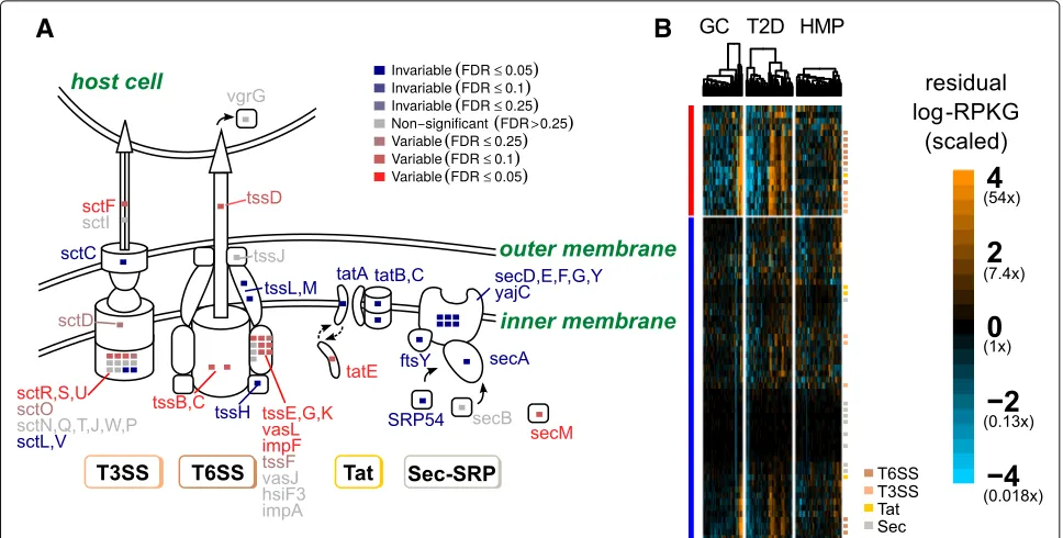
A
B
Fig. 4Variable and invariable gene families involved in bacterial secretion separate by gene function.aSchematic diagram showing the type III (T3SS), type VI (T6SS), Sec, and Tat secretion system gene families measured in this dataset. Gene families are color-coded by whether they were variable (red), invariable (blue), or neither (gray), with strength of color corresponding to the FDR cutoff (color intensity).Insetsshow a summary of how many gene families in KEGG modules corresponding to a particular secretion system were variable or invariable and at what level of significance.bHeatmaps showing scaled residual log-RPKG for gene families (rows) involved in bacterial secretion. Variable (red) and invariable (blue) gene families were clustered separately, as were samples within a particular study (columns). log-RPKG values were scaled by the expected variance from the negative binomial null distribution. Genes in specific secretion systems are annotated withcolored squares(T6SS:red-orange; T3SS: orange; Tat:yellow; Sec:grey)
of TLR4-dependent inflammation. Importantly, since the majority of gene families annotated to LPS biosynthesis were invariable, this result would have been missed by considering the pathway as a unit.
Many invariable gene families are deeply conserved Conservation of gene families across the tree of life is one factor we might expect to affect gene variability. For instance, ribosomal proteins should appear to be invari-able merely because they are shared by all members of a given kingdom of life. To explore the relationship between gene family taxonomic distribution and variabil-ity in abundance across hosts, we constructed trees of the sequences in each KEGG family using ClustalOmega and FastTree. We then calculated phylogenetic distribution (PD), using tree density to correct for the overall rate of evolution (Dongying Wu, personal communication, 2015) (Fig. 6a).
Overall, invariable gene families with below-median PD tended to be involved in carbohydrate metabolism and signaling. Specifically, these 2046 gene families were enriched for the pathways “two-component signaling” (q = 1.5 × 10⁻¹⁵), “starch and sucrose metabolism” (q = 1.8× 10⁻³), “amino sugar and nucleotide sugar
metabolism” (q = 0.063), “ABC transporters” (q =
2.4×10⁻⁵), and “glycosaminoglycan [GAG] degradation” (q = 0.053), among others (Additional file 10). Enriched modules included a two-component system involved in sporulation control (q=0.018), as well as transporters for rhamnose (q = 0.14), cellobiose (q = 0.14), andα- and β-glucosides (q=0.14 andq=0.19, respectively). These results are consistent with the hypothesis that one func-tion of the gut microbiome is to encode carbohydrate-utilization enzymes the host lacks [55]. Additionally, recent experiments showed that the major gut commensal Bacteroides thetaiotaomicroncontains enzymes adapted to the degradation of sulfated glycans including GAGs [56, 57] and that many Bacteroides species can in fact use the GAG chondroitin sulfate as a sole carbon source [58].
A
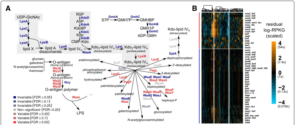
B
Fig. 5Central Kdo and lipid A biosynthesis is invariable, but many genes involved in covalent modifications to LPS are variable.aPathway schematic showing a selection of measured gene families involved in lipopolysaccharide metabolism. Gene families are color-coded by whether they were variable (red) or invariable (blue), with strength of color corresponding to the FDR cutoff (color intensity). Central Kdo and lipid A metabolism is highlighted inlight gray. Abbreviated metabolites are (GlcNAcN-acetylglucosamine), (Kdoketodeoxyoctonate), (R5Pribose-5-phosphate), (S7P sedoheptulose-7-phosphate), (GMHglyceromannoheptose), (aminoarabinose4-amino-4-deoxy-L-arabinose).bHeatmaps showing scaled residual log-RPKG for gene families (rows) involved in lipopolysaccharide metabolism, as in Fig. 4
strain-specific manner, using a wholly separate set of data [59]. Finally, gene families described as “hypothetical” were enriched in the high-PD but variable gene set (p = 2.4×10⁻⁸, odds ratio = 2.2) and depleted in the low-PD
but invariable set (p=5.4×10⁻¹³, odds ratio = 0.41).
Transporters show strain-specific variation in copy number across different human gut microbiomes [59], and analyses by Turnbaugh et al. identified membrane transporters as enriched in the “variable” set of func-tions in the microbiome [12]. However, we mainly found transporters enriched among gene families with simi-lar abundance across hosts, despite being phylogeneti-cally restricted (low-PD but invariable genes; Additional file 11). Part of this difference is likely due to our strati-fying by phylogenetic distribution, a step previous studies did not perform.
Proteobacteria are the major source of variable genes To assess which taxa contributed these variable and invariable genes, we first computed correlations between phylum relative abundances (predicted using MetaPhlAn2 [60]) and gene family abundances. Specifically, we used a permutation test based on partial Kendall’sτ correlation. This test is rank-based and thus distribution-agnostic, handles ties (unlike Spearman’sρ), and accounts for study-to-study variation by using partial correlation (see the “Methods” section). The resultingpvalues were corrected for multiple testing using theqvalue method and thresh-olded at an FDR ofq ≤ 0.05. Based on these results, we then determined whether phyla were enriched for variable
or invariable genes by Fisher’s exact test (Bonferroni-correctedp ≤ 0.05). This analysis revealed that the pre-dicted abundance of Proteobacteria was strongly enriched for correlations with variable gene families (Bonferroni-corrected p ≤ 10−8): Fig. 7b). The abundance of the
archaeal phylum Euryarchaeota was also enriched for cor-relations with variable gene families, to a lesser extent (Bonferroni-correctedp≤10−4).
Fig. 6Phylogenetic distribution (PD) of gene families partially explains gene family variability. Scatter plot shows log10PD (x-axis) vs. log10residual variance statistic (y-axis).Red pointswere significantly variable andblue pointswere significantly invariable. Gene families in specific functional groups are also highlighted in different colors, specifically the bacterial ribosome (green), the type VI secretion system (or “T6SS”;orange), the KinABCDE-Spo0FA sporulation control two-component signaling system (yellow), and hypothetical genes (tan squares). Gene families that were significantly invariable (ribosome and sporulation control) or significantly variable (hypothetical genes and the T6SS) at an estimated 5% FDR are outlined in black. The bacterial ribosome, as expected, had very high PD and was strongly invariable. The type VI secretion system genes, in contrast, were conserved but variable, and some genes involved in the Kin-Spo sporulation control two-component signaling pathway had low PD but were invariable. Only gene families with at least one annotated bacterial or archaeal homolog are shown
It has been proposed that a small number of “enterotypes” may exist in the human gut microbiome, each with distinct taxonomic composition [25, 26]. Most recently, abundances of the taxaRuminococcaceae, Bacteroides, and Prevotella were found to explain the most taxonomic variation across individuals [28]. These enterotypes appeared to be linked to long-term diet, with Prevotellahighest in individuals with the most carbohy-drate intake andBacteroidescorrelating with protein and animal fat. However, while these clades contributed most to taxonomic variation, in our study, all were actually depletedfor associations with variable genes. In contrast, the Proteobacterial familyEnterobacteriaceae(Additional file 13: Figure S12B), and to a lesser extent, Gammapro-teobacteria in general (Additional file 13: Figure S12C) were much more likely to be associated with variable gene families. Similar results were also obtained using the cen-tered log-ratio (clr) transform to correct potential com-positionality artifacts (see Additional file 14: Figure S16). This suggests that compared to previously identi-fied enterotype marker taxa, levels of Proteobacteria,
and potentially Euryarchaeota, better explain person-to-person variation in gut microbial gene function. These less abundant phyla were missed in enterotype studies, likely because enterotypes were identified by methods that will tend to weight higher-abundance taxa more, and enterotypes were identified from taxonomic, not func-tional data.
Because Proteobacteria are a relatively well-annotated yet low-abundance phylum, we explored whether either of these characteristics explain their association with variable genes. Importantly, genes correlated with Actinobacteria did not tend to be variable, even though Proteobacteria and Actinobacteria had similar levels of abundance (Additional file 12: Figure S10). Also, while they were comparatively low abundance compared to Bacteroidetes or Firmicutes, Proteobacteria were also generally not close to the limit of detection when present: Proteobacterial relative abundance was more than 0.18 in 90% of samples, whereas MetaPhlAn2 was able to detect taxa with relative abundances of only 0.0004% in our data. Low abundance therefore does not appear to explain this association.
The number of phyla present in our data was not enough to determine whether there was any trend for low-prevalence or low-abundance taxa to be more cor-related with variable genes. To answer this question, we conducted the same analysis with bacterial and archaeal taxa at the family level. However, when considering the 30 families with significant enrichments for (in)variable or non-significant gene families, there was no signifi-cant association between the degree of enrichment for variable genes and either prevalence (r = −0.07, p = 0.72) or abundance (r = −0.1, p = 0.58) (Additional file 13: Figure S12D-E). In fact,Enterobacteriaceae, a Pro-teobacterial family, was significantly enriched for corre-lations with variable genes despite a prevalence of 86%, in the top 25% of all families detected. Thus, preva-lence and abundance do not explain the variability of Proteobacterial genes.
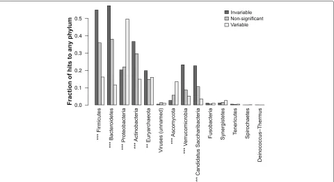
Fig. 7Variable gene families correlate with the predicted abundance of Proteobacteria.Bar plotsgive the fraction of gene families in each category (significantly invariable, non-significant, and significantly variable, 5% FDR) that were significantly correlated to predicted relative abundances of phyla, as assessed by MetaPhlAn2, using partial Kendall’sτto account for study effects and a permutation test to assess significance.Asterisksgive the level of significance by chi-squared test of non-random association between gene family category and the number of significant associations. (***p≤10−8by chi-squared test after Bonferroni correction; **p≤10−4)
repeated the entire statistical test on a subset of genes, sampling one part phylum-specific genes drawn equally from Proteobacteria, Actinobacteria, Firmicutes, and Eur-yarchaeota, and one part genes annotated to all four phyla (see the “Methods” section). Again, Proteobacteria-and Euryarchaeota-specific genes were significantly vari-able more often than those from either Actinobacteria or Firmicutes (Additional file 15: Figure S13B). We there-fore concluded that phylum abundance and annotation bias do not explain the enrichment of variable genes in Proteobacteria.
Finally, variable genes also do not appear to be biomark-ers for either taxonomic statistics or measured host char-acteristics. To explore this question, we used the same two-sided partial Kendall’sτ test as above. With regard to taxonomic statistics, we testedα-diversity (measured by Shannon entropy), the Bacteroidetes/Firmicutes ratio, and average genome size (AGS): however, all of these correlated more often with invariable gene families (see Additional file 9, Additional file 13: Figure S12A). For host characteristics, we selected body mass index, sex, and age, which were measured in all three studies we ana-lyzed. None of these variables correlated significantly with anyvariable gene family abundances, even at a 25% false discovery rate.
One study (GC) measured blood levels of three inflam-matory markers, TNFα, IL-1, and CD163, which did not correlate with Proteobacterial abundance in this study (Holm-corrected p value >0.2, Kendall’s τ). However, other inflammatory markers directly linked to changes in Proteobacterial abundance (e.g., IgA, 10, and IL-17, reviewed in [32]) were not measured in this panel. These results suggest that major correlates of variation in microbiota gene levels, possibly including diet and specific inflammatory markers, remain to be measured.
Bacterial phyla have unique sets of variable genes
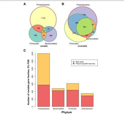
agree, but the reverse was true for variable gene families: 19.4% of gene families that were invariable in one phy-lum were invariable in all, compared to just 0.34% (eight genes) in the variable set (Fig. 8a, b). This trend was robust to the FDR cutoff (Additional file 16: Figure S14A–B). Gene families invariable in all four phyla were enriched for basal cellular machinery, as expected (Additional file 17: C–D).
The relationship between phylum-specific and over-all gene family abundance variability differed by phylum. Proteobacteria-specific variable gene families tended to be variable overall (59%), whereas the proportions of
gene families that were also variable overall were much lower for Bacteroidetes- (12%), Firmicutes- (29%), and Actinobacteria-specific (18%) gene families (Fig. 8c). This supports the hypothesis that Proteobacterial abundance is a dominant factor influencing functional variability in the human gut microbiome. It further suggests that many overall-variable gene families are not only merely markers for the amount of Proteobacteria (or some other phylum) but are also variable at finer taxonomic levels, such as the species or even the strain level [59, 65].
Comparing the two dominant phyla in the gut, Bac-teroidetes and Firmicutes, we further observe that the
A
C
B
overall proportions of variable and invariable fami-lies were similar across pathways, with some inter-esting exceptions. For example, LPS biosynthesis had more invariable gene families in Bacteroidetes than in Firmicutes, which we expected given that LPS is pri-marily made by Gram-negative bacteria. Conversely, both two-component signaling and the PTS system had many more invariable gene families in Firmicutes than in Bac-teroidetes (Additional file 16: Figure S14C). However, phylum-specific variable gene families tended not to over-lap (median overover-lap, 0%, compared to 46% for invari-able gene families). This was even true for pathways where the overall proportion of variable and invariable gene families was similar, such as cofactor and vita-min biosynthesis and central carbohydrate metabolism (Additional file 16: Figure S14D). Thus, unique genes within invariable pathways vary in their abundance across microbiome phyla.
Furthermore, the enriched biological functions of the phylum-specific variable gene families differed by phylum (Additional file 18). For instance, Proteobacterial-specific variable gene families were enriched (Fisher’s test enrich-mentq=0.13) for the biosynthesis of siderophore group nonribosomal peptides, which may reflect the importance of iron scavenging for the establishment of both pathogens (e.g.,Yersinia) and commensals (e.g.,Escherichia coli) [66]. Another phylum-specific variable function appeared to be the type IV secretion system (T4SS) within Firmi-cutes (q =0.021). Homologs of this specialized secretion system are involved in a wide array of biochemical interac-tions, including the conjugative transfer of plasmids (e.g., antibiotic-resistance cassettes) between bacteria [67]. We conclude that our approach enables the identification of substantial variation within all four major bacterial phyla in the gut, much of which is not apparent when data are analyzed at broader functional resolution or without stratifying by phylum.
Discussion
This study presents a novel test for genes whose abun-dances are significantly more or less variable across indi-viduals than expected. This test, which we call CCoDA, provides a finer resolution and more statistically grounded estimate of “functional redundancy” [68] than was pre-viously possible in the human microbiome. CCoDA dif-fers from earlier approaches to quantifying variability in microbiome function in several key ways. First, we focus explicitly on the variability of gene family abun-dance, not differences in mean abundance between prede-fined groups, as has been done to reveal pathways whose abundance differs between body sites [69] or disease states [6].
Second, by using a null distribution based on the nega-tive binomial, our model accounts for stochastic variation
in gene family abundance between individuals caused by sampling. This parametric bootstrap null is more compu-tationally intensive than previous approaches. However, the use of such a null allows us much better control over the false discovery rate than previous approaches that dichotomized gene families based on binary pres-ence/absence [12]. Dichotomizing in this way may be acceptable for small datasets. However, based on the data used here, dichotomizing would classify 12% of sig-nificantly invariable (FDR ≤ 0.05) gene families and, more problematically, 85% of non-significant gene fam-ilies (q ≥ 0.25) as part of the “variable” metagenome. This problem is not easily avoided by picking a dif-ferent presence/absence cutoff (see Additional file 19: Figure S15).
A third important aspect of our method is that the underlying model accounts for the mean-variance rela-tionship in count data and corrects for systematic biases between studies. While estimating this mean-variance relationship accurately requires a significant sample size (the best results in simulations were obtained withn≥40 per study), CCoDA can identify individual gene families as well as pathways that break this overall trend. Because we account for the mean-variance relationship, we iden-tify different variable pathways than the previous studies that relied on the sample variance only [13]. Additionally, our major findings are robust when we apply the cen-tered log-ratio transform (see Additional file 14: Figure S16). Importantly, unlike previous work, CCoDA tends to call pathways that are well-conserved across prokaryotes invariable (for example, the Sec general secretory system; see Fig. 6). This suggests that this method better captures biological intuition about meaningful variation. Fourth, the null distribution is estimated from the shotgun data and does not require comparisons to sequenced genomes [12]. Finally, unlike previous approaches, CCoDA can be used for meta-analysis, integrating data from multiple different populations.
source [56], and the metabolism of resistant starch in general is thought to be a critical function of the omnivo-rous mammalian microbiome [55]. These results suggest that our method identifies protein-coding gene families that contribute to fitness of symbionts within the gut. Finally, we found a number of invariable gene families whose function is not yet annotated. These gene families may represent functions that are either essential or pro-vide advantages for life in the gut and may therefore be particularly interesting targets for experimental follow-up (e.g., assessing whether strains in which these gene fam-ilies have been knocked out in fact have slower growth rates, either in vitro or in the gut).
We also identified significantly variable gene fami-lies, including enzymes involved in carbon metabolism, specialized secretion systems such as the T6SS, and LPS biosynthetic genes. Proteobacteria, rather than Bac-teroidetes or Firmicutes, emerge as a major source of variable genes, including some genes whose abundance also varied within the Proteobacteria (e.g., T6SS). Since Proteobacteria have been linked to inflammation and metabolic syndrome [32], we speculate that inflamma-tion may be one variable influencing funcinflamma-tions in the gut microbiome. Some variable genes, including many of unknown function, had surprisingly broad phylogenetic distributions.
Variable gene families have a variety of ecological inter-pretations, e.g., first-mover effects, drift, host demogra-phy, and selection within particular gut environments. Computationally distinguishing among these possibilities is likely to present challenges. For example, distinguishing selection from random drift will probably require longi-tudinal data and appropriate models. Separating effects of host geography, genetics, medical history, and lifestyle will be possible only when richer phenotypic data is available from a more diverse set of human populations. To con-trol for study bias and batch effects, it will be important to include multiple sampling sites within each study.
While statistical tests focused on differences in vari-ances are not yet common throughout genomics, there is recent precedent using this type of test to quantify the gene-level heterogeneity in single-cell RNA sequenc-ing data [19, 20] and to identify variance effects in genetic association data [70]. Like Vallejos et al. [20], we model gene counts using the negative binomial distribu-tion and identify both significantly variable and invariable genes. In contrast, we frame our method as a frequen-tist hypothesis test as opposed to a Bayesian hierarchical model. Our method also accounts for study-to-study vari-ation. Also, unlike previous approaches in this domain, CCoDA does not require biological noise to be explic-itly decomposed from technical noise. Thus, our method does not require the use of experimentally spiked-in con-trols, which are not present in most experiments involving
sequencing of the gut microbiome. Instead, we detect differences from the average level of variability using a robust non-parametric estimator, which we show through simulation leads to correct inferences under reasonable assumptions.
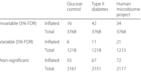
Our null model does not explicitly account for zero-inflation, that is, the presence of more zeros than predicted by the negative binomial model; models incor-porating zero-inflation have been proposed for taxo-nomic microbiome data [71–73]. However, only 1–2% of gene families showed significant zero-inflation, and our method tended to call these genes non-significant (Table 2). This suggests that zero-inflation may not be as severe a problem for measuring gene family abun-dance as it is for measuring microbial species. However, if applied to a dataset where measurements were expected to be more sparse, the method could be modified to generate the null from a zero-inflated negative binomial distribution.
A statistical method for detecting significant (in)variability similar to the one we present here could also be applied to other biomolecules measured in counts, such as metabolites, proteins, or transcripts. Performing such analyses on human microbiota would reveal pat-terns in the variability in the usage of particular genes, reactions, and pathways, which would expand on our investigation of potential usage based on presence in the DNA of organisms in host stool. Integrating the results of these analyses could also further help to validate or inter-pret the functional variability we observe in this dataset. For example, mass spectrometry methods that can resolve differently modified LPS molecules could reveal whether the variation we observe at the metagenomic level is also seen across LPS molecules with different immunogenic properties. Of course, we would also expect that key functions provided by the microbiome would be highly regulated at the level of transcript or protein abundance. Integrating transcript and/or protein variability with
Table 2Number of genes (with at least one bacterial/archaeal representative) with significant zero-inflation in each dataset, q≤0.05
Glucose control
Type II diabetes
Human microbiome project
Invariable (5% FDR) Inflated 16 42 34
Total 3768 3768 3768
Variable (5% FDR) Inflated 6 11 21
Total 1218 1218 1215
Non-significant Inflated 55 67 72
DNA variability would allow us to come up with more precise hypotheses about which functions are effectively constitutive and which are more strongly modulated by the gut environment.
Another important extension will be to generalize our method for comparing hosts from different predefined groups (e.g., disease states, countries, diets) to identify gene families that are invariable in one group (e.g., healthy controls) but variable in another (e.g., patients), analo-gously to recent methods for the analysis of single-cell RNAseq [21] and GWAS [70] data. In particular, gene families whose variance differs between case and control populations could point to heterogeneity within com-plex diseases, interactions between the microbiome and latent variables (e.g., environmental or genetic), and/or differences in selective pressure between healthy and diseased guts. Investigating group differences in func-tional variability could thereby allow the detection of different trends from the more common comparison of means.
Conclusions
We present a statistical test for variability called CCoDA that can integrate data from multiple studies to identify individual variable and invariable gene families. Simula-tions reveal CCoDA has high accuracy and power across a range of realistic scenarios. Applying this test to shot-gun metagenomes from healthy human gut microbiota, we uncovered thousands of variable gene families whose abundances were more variable than expected. In general, more conserved genes tended to be less variable, but sig-nificantly variable genes also included some with relatively broad phylogenetic distributions. Finally, while the phyla Bacteroidetes and Firmicutes varied substantially between healthy individuals, consistent with previous studies of the human gut microbiome, we found that these phyla were actually depleted for associations with variable genes. The same was true for genera and families used to define “enterotypes.” Instead, a less abundant phylum, Proteobac-teria, contributed most to functional variation in this population. These results argue that gene function in the healthy human gut microbiome may be more variable than previously assumed and that the major axes of taxo-nomic variation in microbiota do not necessarily capture the most variation in function.
Methods
Overview
CCoDA takes as input reads that have been mapped to a reference library of gene families, yielding counts of gene families in each sample (see “Data collection and pro-cessing” in the “Methods” section). The following general process is then applied (see also Additional file 2: Figure S2 for a graphical depiction):
• Counts are normalized for genome size and gene length, yielding reads per kilobase of genome
equivalent (RPKG) (the “Data normalization” section)
• Confounding factors, like study-to-study variation, are regressed out using a linear model (the “Model fitting to correct for covariates” section)
• The variance of the resulting residuals is calculated per gene (the “Model fitting to correct for covariates” section);
• A null distribution is generated (the “Modeling residual variances under the null distribution” section):
– An overdispersion parameterkygiving the mean-variance relationship is fit (per studyy) – This parameter, along with the estimated
means of each gene, is used to generate null count data via parametric bootstrap – The first four steps are repeated on the null
count data to obtain null residual variances for each gene
– Repeat until the desired number of bootstrap samples is reached
• Based on the resulting null distribution,p-values are calculated and corrected for multiple testing.
Data collection and processing
Stool metagenomes from healthy human guts were obtained from three sources:
1. Two American cohorts from the Human
Microbiome Project [13],n=42samples selected, 2. A Chinese cohort from a case-control study of type II
diabetes (T2D) [33],n=44samples from controls with neither type II diabetes nor impaired glucose tolerance, and
3. A European cohort from a case-control study of glucose control [34],n=37samples from controls with normal glucose tolerance.
These studies were chosen because they contained large cohorts of healthy individuals and were publicly available at the time at which we began this study. Samples (see Additional file 20 for SRA IDs) were chosen to have at least 1.5×10⁷reads and mode average quality scores≥20
(estimated via FastQC [74]). For consistency, each sample was rarefied to a depth of 1.5×10⁷ reads, and as reads
from HMP were particularly variable in length, they were trimmed to a uniform length of 90 bp.
After downloading these samples from NCBI’s
a particular protein family were selected based on the average read length of each sample as described [35]. The KEGG Orthology database was chosen because it annotates a large number of bacteria and archaea, including many species observed in the human gut, and covers a wide range of gene families, including metabolic enzymes, signaling proteins, and virulence factors.
Data normalization
The gene family counts were normalized for two con-founders:
1. Average family length (AFL) or the average length of the matched genes within a gene family
2. Average genome size (AGS) or the estimated average genome length based on single-copy universal marker genes (estimated using MicrobeCensus: [36] http://github.com/snayfach/MicrobeCensus).
Normalization for these two factors yielded abundance values in units of RPKG or reads per kilobase of genome equivalents [36].
These RPKG abundance values were strictly positive with a long right tail and highly correlated with the vari-ances (Spearman’sr = 0.99). This strong mean-variance relationship is likely simply because these abundances are derived from counts that are either Poisson or negative binomially distributed. We therefore took the natural log of the RPKG values as a variance-stabilizing transforma-tion. Because log 0 is infinite, we added a pseudocount before normalizing the counts and taking the log trans-form. Since there is no AFL when there are no reads for a given gene family in a given sample, we imputed it in those cases using the average AFL across samples.
Model fitting to correct for covariates
We fit a linear model to the data matrix of log-RPKGD of log-RPKG described above, withngene families bym samples. The purpose of this linear model is to regress out variation caused by factors we were not interested in (here, study-to-study variation and per-gene-family mean values):
Dg,s=μg+
y∈Y
Iy,sβg,y+g,s (3)
whereg ∈[1,n] is a particular gene family,s ∈[1,m] is a particular sample,μgis estimated by the grand (i.e.,
over-all) mean of log-RPKG
sDg,s
m for a given gene family g, Y is the set of studies, Iy,s is an indicator variable val-ued 1 if samplesis in studyyand 0 otherwise,βg,y is a mean offset for gene familyg in study y, and the resid-ual for a given gene family and sample are given by g,s. For each gene family, the variance across samples of these g,s, which we term the “residual variance” orVg, was our
statistic of interest. In this case, residuals can be obtained simply by subtracting the per-dataset means from each gene family.
Overall trends in these data are explained well by this model, with an R2 = 0.20. The residuals, which are approximately symmetrically distributed around 0, repre-sent variation in gene abundance not due to study effects.
Modeling residual variances under the null distribution Having calculated this statistic Vg for each gene family g, we then needed to compare this statistic to its distri-bution under a null hypothesisH0. This required us to
model what the data would look like if in fact there were no surprisingly variable or invariable gene families. To do this, we used the negative binomial distribution to model the original count data (before adding pseudocounts and normalization to obtain RPKG).
The negative binomial distribution is commonly used to model count data from high-throughput sequencing. It can be thought of as a mixture of Poisson distributions with different means (themselves following a Gamma distribution). Like the Poisson distribution, the negative binomial distribution has an intrinsic mean-variance rela-tionship. However, instead of a single parameter control-ling both mean and variance as in the Poisson, the negative binomial has two, a mean parameter μ and a “size” or “overdispersion” parameterk.kis defined byk = σ2μ−2μ.
(If the sample mean is plugged into μ and the sample variance into σ2, this equation also gives a
method-of-moments estimator for k.) k ranges from (0,∞), with smaller values corresponding to more overdispersion (i.e., higher variance given the mean) and larger values approaching, in the limit, the Poisson distribution.
To model the case where no gene family has unusual variance given its mean value (i.e., our null hypothesis), we assumed that the data were negative binomially dis-tributed with the observed means μg,y for each gene g and study y, but where the amount of overdispersion was modeled with a single size parameter ky for each study y. This has similarities to previous approaches to model RNAseq distributions [22, 39, 76] and to identify (in)variable genes from single-cell RNAseq data [20] (see also the “Discussion” section).
H0: Vg =Vg|Dg,s∼NB
μg,y, ky
Halt: Vg=Vg|Dg,s∼NB
μg,y, ky
kernel density estimate to the log-transformedkg,yvalues, and then finding thekyvalue that gave the highest density. (From simulations, we found that the mode method-of-moments was more robust than the median or harmonic mean; see Additional file 21: Figure S3. We use the har-monic mean here because the arithmetic mean ofkg,y is highly unstable, probably because the distribution ofkhas a long right-hand tail [77]).
Having estimated ky and the per-gene means μg, we can now easily generate count data under this null distri-bution, yielding a parametric bootstrap null. These null count data are then treated identically to the real data: we add a pseudocount and normalize by AFL and AGS, fit the above linear model, and obtain null residual variancesV0
g exactly as before.
Once the null is generated, statistical significance was obtained by a two-tailed test:
pg=
# V
0
g −Vg0 Vg0
2
≥ Vg−Vg0 Vg0
2
+1
B+1
Here,Brefers to the number of null test statisticsV0
g (in this case,B = 750), and the overlined test statistics refer to their mean across the null distribution.
The resultingpvalues were then corrected for multiple testing by converting to FDR q-values using the proce-dure of Storey et al. [78] as implemented in theqvalue package in R [79].
An alternative approach to determining significance is based on the bootstrap. While using a parametric null distribution allows us to explicitly model the null hypoth-esis, it also breaks the structure of covariance between gene families, which may be substantial because genes are organized into operons and individual genomes within a metagenome. This structure can, optionally, be restored using a strategy outlined by Pollard and van der Laan [80]. Instead of using the test statisticsV0
g obtained under the parametric null as is, we can use these test statistics to cen-ter and scale non-parametric bootstrap test statisticsVg, which we derive from applying a cluster bootstrap with replacement from the real data and then fitting the above linear model (3) to the resampled data to obtain bootstrap residual variances:
V0
g =
⎛ ⎝ ⎛
⎝Vg−Vg sd
Vg
⎞
⎠×sdV0
g
⎞ ⎠+V0
g
A similar non-parametric bootstrap approach has pre-viously been successfully applied to testing for differences in gene expression [80].
Visualization
As expected, when the residuals are plotted in a heatmap as in Additional file 6: Figure S7, variable gene fami-lies were generally brighter (i.e., more deviation from the mean) than invariable gene families, though not exclu-sively: this is because our null distribution, unlike the visualization, models the expected mean-variance rela-tionship. We visualized this information by scaling each gene family by its expected standard deviation under the negative binomial null (i.e., by the mean root variance
b∈[1,B]
V0
gb/B) (Additional file 7: Figure S8).
In Fig. 4, for comparability with existing literature, gene families in the T6SS were named by mapping to the COG IDs used in Coulthurst [47], except when multiple KOs mapped to the same COG ID; in these cases, the original KO gene names were kept. Schematics of the T3SS, T6SS, Tat, and Sec pathways were modeled on previous reviews [47, 81, 82] and on the KEGG database [75]. The pathway diagram in Fig. 5 is based on representations in the KEGG database [75], MetaCyc [83], and reviews by Wang and Quinn [84] and Whitfield and Trent [85]. These reviews were also used to identify KEGG Orthology gene families that were involved in lipopolysaccharide metabolism but not yet annotated under that term.
Power analysis
Statistical tests should have reasonable power (also called “recall”) and controlα, the false positive or type I error rate, at the desired level (e.g., 5% for apvalue cutoff of 0.05). Our test controlsα as expected if the correct size parameterkis estimated from the data (Additional file 21: Figure S3a-b). Estimating this parameter accurately is dif-ficult, however, particularly for highly over-dispersed data [77], and in this case, we must also estimate this param-eter from a mixture of true positives and nulls. We found that the mode of per-gene-family method-of-moments estimates was more robust to differences in the ratio of variable to invariable true positives (Additional file 21: Figure S3e–g) than the median or harmonic mean (the harmonic mean mirrors the approach in Yu et al. [76]).
(i.e., false positive and false negatives) were calculated by comparing to the known gene family labels from the simulation. Using similar parameters to those estimated from our real data, we saw thatα decreased and power approached 1 with increasing sample size (see Additional file 4: Figure S4) and thatn=120 appeared to be sufficient to achieve control overα.
Calculation of an empirical FDR
Atn = 120, we also noted thatα appeared to be greater for variable vs. invariable gene families (Additional file 5: Figure S5). This could be because accurately detecting additional overdispersion in already over-dispersed data may be intrinsically difficult. Instead of using a single q value cutoff for both variable and invariable genes, we per-formed additional simulations to determine whatqvalue cutoff corresponded to an empirical FDR of 5%. We cal-culated appropriate cutoffs based on datasets with 43% true positives and a variable to invariable gene family ratio ranging from 0.1 to 10, taking the median cutoff value across these ratios (Additional file 10). Using these cutoffs, the overall dataset had 45% true positives and a variable to invariable gene family ratio of 0.43, indicating that these simulations were realistic.
Estimating the phylogenetic distribution of gene families To obtain estimates of the PD of KO gene families, we first obtained sequences of each full-length protein annotated to a particular KO. These sequences were then aligned using ClustalOmega [86]. The resulting multiple align-ments were then used to generate trees via FastTree [87]. For both the alignment and tree building, we used default parameters for homologous proteins.
For all gene families represented in at least five dif-ferent archaea and/or bacteria (6703 families total), we then computed tree densities, or the sum of edge lengths divided by the mean tip height. Using tree density instead of tree height as a measure of PD corrects for the rate of evolution, which can otherwise cause very highly con-served but slow-evolving families like the ribosome to appear to have a low PD (Dongying Wu, personal commu-nication, 2015). Empirically, this measure is very similar to the number of protein sequences (Additional file 22: Figure S11) but is not as sensitive to high or variable rates of within-species duplication: for example, families such as transposons, which exhibit high rates of duplica-tion as well as copy number variaduplica-tion between species, have a larger number of sequences than even very well-conserved proteins such as RNA polymerase, but have similar or even lower tree densities, indicating that they are not truly more broadly conserved.
Many protein families (8931 families) did not have enough observations to reliably calculate tree density, with almost all of these being annotated in only a single
bacterial/archaeal genome. For these, we predicted their PD by extrapolation. To predict PD, we used a linear model that predicted tree density based on the total num-ber of annotations (including annotations in eukaryotes). In fivefold cross-validation, this model actually had a rel-atively small mean absolute percentage error (MAPE) of 13.1%. We also considered a model that took into account the taxonomic level (e.g., phylum) of the last common ancestor of all organisms in which a given protein family was annotated, but this model performed essentially iden-tically (MAPE of 13.0%). Predicted tree densities are given in Additional file 23. The PD of gene families varied from 1.2 (an iron-chelate-transporting ATPase only annotated inHelicobacter pylori) to 434.9 (therpoEfamily of RNA polymerase sigma factors).
Gene family enrichment
We were interested in whether particular pathways were enriched in several of the gene family sets identified in this work. For subsets of genes (such as those with specifically low PD), a two-tailed Fisher’s exact test (i.e., hypergeomet-ric test) was used instead to look for cases in which the overlap between a given gene set and a KEGG module or pathway was significantly larger or smaller than expected. The background set was taken to be the intersection of the set of gene families observed in the data with the set of gene families that had pathway- or module-level annota-tions.pvalues were converted toqvalues as above. Finally, enrichments were enumerated by selecting all modules or pathways belowq≤0.25 that had positive odds ratios (i.e., enriched instead of depleted).
Associations with clinical and taxonomic variables
We used a general, non-parametric approach to detect association of residual RPKG with clinical and taxonomic variables (e.g., the inferred abundance of a particular phy-lum or other clade via MetaPhlAn2). To take into account potential study effects in clinical and taxonomic vari-ables without using a parametric modeling framework, we used partial Kendall’sτ correlation as implemented in the ppcor package for R [88], coding the study effects as binary nuisance variables.
Kendall’s τ was used instead of Spearman’sρ because while both are correlations based on ranks, Kendall’s τ performs better when many observations have the same rank. This is a particular problem with taxonomic data because many taxa have zero abundance in some samples, making their ranks equal.