www.earth-syst-sci-data.net/7/47/2015/ doi:10.5194/essd-7-47-2015
© Author(s) 2015. CC Attribution 3.0 License.
Global carbon budget 2014
C. Le Quéré1, R. Moriarty1, R. M. Andrew2, G. P. Peters2, P. Ciais3, P. Friedlingstein4, S. D. Jones1, S. Sitch5, P. Tans6, A. Arneth7, T. A. Boden8, L. Bopp3, Y. Bozec9,10, J. G. Canadell11, L. P. Chini12, F. Chevallier3, C. E. Cosca13, I. Harris14, M. Hoppema15, R. A. Houghton16, J. I. House17, A. K. Jain18,
T. Johannessen19,20, E. Kato21,22, R. F. Keeling23, V. Kitidis24, K. Klein Goldewijk25, C. Koven26, C. S. Landa19,20, P. Landschützer27, A. Lenton28, I. D. Lima29, G. Marland30, J. T. Mathis13, N. Metzl31,
Y. Nojiri21, A. Olsen19,20, T. Ono32, S. Peng3, W. Peters33, B. Pfeil19,20, B. Poulter34, M. R. Raupach35,†, P. Regnier36, C. Rödenbeck37, S. Saito38, J. E. Salisbury39, U. Schuster5, J. Schwinger19,20, R. Séférian40,
J. Segschneider41, T. Steinhoff42, B. D. Stocker43,44, A. J. Sutton45,13, T. Takahashi46, B. Tilbrook47,
G. R. van der Werf48, N. Viovy3, Y.-P. Wang49, R. Wanninkhof50, A. Wiltshire51, and N. Zeng52
1Tyndall Centre for Climate Change Research, University of East Anglia, Norwich Research Park,
Norwich NR4 7TJ, UK
2Center for International Climate and Environmental Research – Oslo (CICERO), Oslo, Norway 3Laboratoire des Sciences du Climat et de l’Environnement, Institut Pierre-Simon Laplace,
CEA-CNRS-UVSQ, CE Orme des Merisiers, 91191 Gif sur Yvette Cedex, France
4College of Engineering, Mathematics and Physical Sciences, University of Exeter, Exeter EX4 4QF, UK 5College of Life and Environmental Sciences, University of Exeter, Exeter EX4 4QE, UK 6National Oceanic & Atmospheric Administration, Earth System Research Laboratory (NOAA/ESRL),
Boulder, CO 80305, USA
7Karlsruhe Institute of Technology, Institute of Meteorology and Climate Research/Atmospheric
Environmental Research, 82467 Garmisch-Partenkirchen, Germany
8Carbon Dioxide Information Analysis Center (CDIAC), Oak Ridge National Laboratory, Oak Ridge, TN, USA 9CNRS, UMR7144, Equipe Chimie Marine, Station Biologique de Roscoff, Place Georges Teissier,
29680 Roscoff, France
10Sorbonne Universités (UPMC, Univ Paris 06), UMR7144, Adaptation et Diversité en Milieu Marin,
Station Biologique de Roscoff, 29680 Roscoff, France
11Global Carbon Project, CSIRO Oceans and Atmosphere Flagship, GPO Box 3023, Canberra,
ACT 2601, Australia
12Department of Geographical Sciences, University of Maryland, College Park, MD 20742, USA 13National Oceanic & Atmospheric Administration/Pacific Marine Environmental Laboratory (NOAA/PMEL),
7600 Sand Point Way NE, Seattle, WA 98115, USA
14Climatic Research Unit, University of East Anglia, Norwich Research Park, Norwich NR4 7TJ, UK 15Alfred Wegener Institute Helmholtz Centre for Polar and Marine Research, Postfach 120161,
27515 Bremerhaven, Germany
16Woods Hole Research Center (WHRC), Falmouth, MA 02540, USA
17Cabot Institute, Department of Geography, University of Bristol, Bristol BS8 1TH, UK 18Department of Atmospheric Sciences, University of Illinois, Urbana, IL 61821, USA
19Geophysical Institute, University of Bergen, Allégaten 70, 5007 Bergen, Norway 20Bjerknes Centre for Climate Research, Allégaten 55, 5007 Bergen, Norway
21Center for Global Environmental Research, National Institute for Environmental Studies (NIES),
16-2 Onogawa, Tsukuba, Ibaraki 305-8506, Japan
22Institute of Applied Energy (IAE), Minato-ku, Tokyo 105-0003, Japan 23University of California, San Diego, Scripps Institution of Oceanography, La Jolla,
CA 92093-0244, USA
25PBL Netherlands Environmental Assessment Agency, The Hague/Bilthoven and Utrecht University,
Utrecht, the Netherlands
26Earth Sciences Division, Lawrence Berkeley National Lab, 1 Cyclotron Road, Berkeley,
CA 94720, USA
27Environmental Physics Group, Institute of Biogeochemistry and Pollutant Dynamics, ETH Zürich,
Universitätstrasse 16, 8092 Zurich, Switzerland
28CSIRO Oceans and Atmosphere Flagship, P.O. Box 1538 Hobart, Tasmania, Australia 29Woods Hole Oceanographic Institution (WHOI), Woods Hole, MA 02543, USA 30Research Institute for Environment, Energy, and Economics, Appalachian State University, Boone,
NC 28608, USA
31Sorbonne Universités (UPMC, Univ Paris 06), CNRS, IRD, MNHN, LOCEAN/IPSL Laboratory,
4 Place Jussieu, 75252 Paris, France
32National Research Institute for Fisheries Science, Fisheries Research Agency 2-12-4 Fukuura, Kanazawa-Ku,
Yokohama 236-8648, Japan
33Department of Meteorology and Air Quality, Environmental Sciences Group, Wageningen University,
P.O. Box 47, 6700AA Wageningen, the Netherlands
34Department of Ecology, Montana State University, Bozeman, MT 59717, USA 35ANU Climate Change Institute, Fenner School of Environment and Society, Building 141,
Australian National University, Canberra, ACT 0200, Australia
36Department of Earth & Environmental Sciences, CP160/02, Université Libre de Bruxelles,
1050 Brussels, Belgium
37Max Planck Institut für Biogeochemie, P.O. Box 600164, Hans-Knöll-Str. 10, 07745 Jena, Germany 38Marine Division, Global Environment and Marine Department, Japan Meteorological Agency,
1-3-4 Otemachi, Chiyoda-ku, Tokyo 100-8122, Japan
39Ocean Processes Analysis Laboratory, University of New Hampshire, Durham, NH 03824, USA 40Centre National de Recherche Météorologique–Groupe d’Etude de l’Atmosphère Météorologique
(CNRM-GAME), Météo-France/CNRS, 42 Avenue Gaspard Coriolis, 31100 Toulouse, France
41Max Planck Institute for Meteorology, Bundesstr. 53, 20146 Hamburg, Germany
42GEOMAR Helmholtz Centre for Ocean Research Kiel, Düsternbrooker Weg 20, 24105 Kiel, Germany 43Climate and Environmental Physics, and Oeschger Centre for Climate Change Research, University of Bern,
Bern, Switzerland
44Imperial College London, Life Science Department, Silwood Park, Ascot, Berkshire SL5 7PY, UK 45Joint Institute for the Study of the Atmosphere and Ocean, University of Washington, Seattle, WA, USA
46Lamont-Doherty Earth Observatory of Columbia University, Palisades, NY 10964, USA 47CSIRO Oceans and Atmosphere and Antarctic Climate and Ecosystems Co-operative Research Centre,
Hobart, Australia
48Faculty of Earth and Life Sciences, VU University Amsterdam, Amsterdam, the Netherlands 49CSIRO Ocean and Atmosphere, PMB #1, Aspendale, Victoria 3195, Australia
50National Oceanic & Atmospheric Administration/Atlantic Oceanographic & Meteorological Laboratory
(NOAA/AOML), Miami, FL 33149, USA
51Met Office Hadley Centre, FitzRoy Road, Exeter EX1 3PB, UK
52Department of Atmospheric and Oceanic Science, University of Maryland, College Park, MD 20742, USA †deceased
Correspondence to: C. Le Quéré ([email protected])
Received: 5 September 2014 – Published in Earth Syst. Sci. Data Discuss.: 21 September 2014 Revised: 18 March 2015 – Accepted: 20 March 2015 – Published: 8 May 2015
Abstract. Accurate assessment of anthropogenic carbon dioxide (CO2) emissions and their redistribution
fuel combustion and cement production (EFF) are based on energy statistics and cement production data,
re-spectively, while emissions from land-use change (ELUC), mainly deforestation, are based on combined
ev-idence from land-cover-change data, fire activity associated with deforestation, and models. The global at-mospheric CO2 concentration is measured directly and its rate of growth (GATM) is computed from the
an-nual changes in concentration. The mean ocean CO2sink (SOCEAN) is based on observations from the 1990s,
while the annual anomalies and trends are estimated with ocean models. The variability inSOCEAN is
eval-uated with data products based on surveys of ocean CO2 measurements. The global residual terrestrial CO2
sink (SLAND) is estimated by the difference of the other terms of the global carbon budget and compared to
results of independent dynamic global vegetation models forced by observed climate, CO2, and
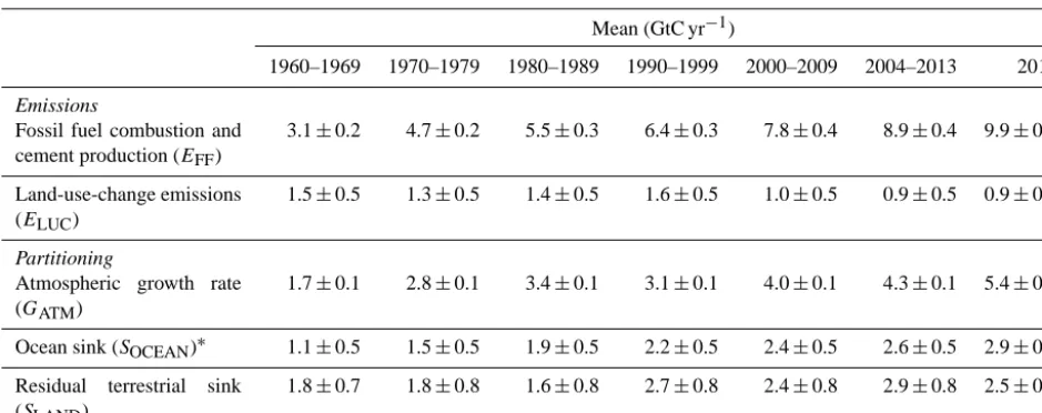
land-cover-change (some including nitrogen–carbon interactions). We compare the mean land and ocean fluxes and their variability to estimates from three atmospheric inverse methods for three broad latitude bands. All uncertain-ties are reported as±1σ, reflecting the current capacity to characterise the annual estimates of each component of the global carbon budget. For the last decade available (2004–2013), EFF was 8.9±0.4 GtC yr−1,ELUC
0.9±0.5 GtC yr−1,GATM 4.3±0.1 GtC yr−1,SOCEAN 2.6±0.5 GtC yr−1, andSLAND2.9±0.8 GtC yr−1. For
year 2013 alone,EFFgrew to 9.9±0.5 GtC yr−1, 2.3 % above 2012, continuing the growth trend in these
emis-sions,ELUCwas 0.9±0.5 GtC yr−1,GATMwas 5.4±0.2 GtC yr−1,SOCEANwas 2.9±0.5 GtC yr−1, andSLAND
was 2.5±0.9 GtC yr−1.G
ATMwas high in 2013, reflecting a steady increase inEFFand smaller and opposite
changes betweenSOCEANandSLANDcompared to the past decade (2004–2013). The global atmospheric CO2
concentration reached 395.31±0.10 ppm averaged over 2013. We estimate thatEFFwill increase by 2.5 % (1.3–
3.5 %) to 10.1±0.6 GtC in 2014 (37.0±2.2 GtCO2yr−1), 65 % above emissions in 1990, based on projections
of world gross domestic product and recent changes in the carbon intensity of the global economy. From this pro-jection ofEFFand assumed constantELUCfor 2014, cumulative emissions of CO2will reach about 545±55 GtC
(2000±200 GtCO2) for 1870–2014, about 75 % fromEFFand 25 % fromELUC. This paper documents changes
in the methods and data sets used in this new carbon budget compared with previous publications of this living data set (Le Quéré et al., 2013, 2014). All observations presented here can be downloaded from the Carbon Dioxide Information Analysis Center (doi:10.3334/CDIAC/GCP_2014).
1 Introduction
The concentration of carbon dioxide (CO2) in the
atmo-sphere has increased from approximately 277 parts per mil-lion (ppm) in 1750 (Joos and Spahni, 2008), the beginning of the Industrial Era, to 395.31 ppm in 2013 (Dlugokencky and Tans, 2014). Daily averages went above 400 ppm for the first time at Mauna Loa station in May 2013 (Scripps, 2013). This station holds the longest running record of direct measure-ments of atmospheric CO2 concentration (Tans and
Keel-ing, 2014; Fig. 1). The atmospheric CO2increase above
pre-industrial levels was initially, primarily, caused by the release of carbon to the atmosphere from deforestation and other land-use-change activities (Ciais et al., 2013). While emis-sions from fossil fuel combustion started before the Industrial Era, they only became the dominant source of anthropogenic emissions to the atmosphere from around 1920 and their rel-ative share has continued to increase until present. Anthro-pogenic emissions occur on top of an active natural carbon cycle that circulates carbon between the atmosphere, ocean, and terrestrial biosphere reservoirs on timescales from days to millennia, while exchanges with geologic reservoirs occur at longer timescales (Archer et al., 2009).
The global carbon budget presented here refers to the mean, variations, and trends in the perturbation of CO2in the
atmosphere, referenced to the beginning of the Industrial Era. It quantifies the input of CO2to the atmosphere by emissions
from human activities, the growth of CO2in the atmosphere,
and the resulting changes in the storage of carbon in the land and ocean reservoirs in response to increasing atmospheric CO2levels, climate and climate variability, and other
anthro-pogenic and natural changes (Fig. 2). An understanding of this perturbation budget over time and the underlying vari-ability and trends of the natural carbon cycle are necessary to understand the response of natural sinks to changes in cli-mate, CO2and land-use-change drivers, and the permissible
emissions for a given climate stabilisation target.
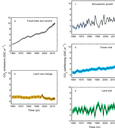
The components of the CO2budget that are reported
an-nually in this paper include separate estimates for (1) the CO2emissions from fossil fuel combustion and cement
pro-duction (EFF; GtC yr−1), (2) the CO2 emissions resulting
from deliberate human activities on land leading to land-use change (LUC;ELUC; GtC yr−1), (3) the growth rate of CO2
in the atmosphere (GATM; GtC yr−1), and the uptake of CO2
by the “CO2sinks” in (4) the ocean (SOCEAN; GtC yr−1) and
(5) on land (SLAND; GtC yr−1). The CO2 sinks as defined
here include the response of the land and ocean to elevated CO2and changes in climate and other environmental
1960 1970 1980 1990 2000 2010 300
310 320 330 340 350 360 370 380 390 400 410
Time (yr)
Atmospheric CO
2
concentration (ppm)
NOAA/ESRL (Dlugokencky & Tans, 2014)
Scripps Institution of Oceanography (Keeling et al., 1976)
Figure 1. Surface average atmospheric CO2 concentration,
de-seasonalised (ppm). The 1980–2014 monthly data are from NOAA/ESRL (Dlugokencky and Tans, 2014). The 1980–2014 esti-mate is an average of direct atmospheric CO2measurements from
multiple stations in the marine boundary layer (Masarie and Tans, 1995). The 1958–1979 monthly data are from the Scripps Institu-tion of Oceanography, based on an average of direct atmospheric CO2measurements from the Mauna Loa and South Pole stations
(Keeling et al., 1976). To take into account the difference of mean CO2between the NOAA/ESRL and the Scripps station networks
used here, the Scripps surface average (from two stations) was har-monised to match the NOAA/ESRL surface average (from multiple stations) by adding the mean difference of 0.542 ppm, calculated here from overlapping data during 1980–2012. The mean seasonal cycle was removed from both data sets.
EFF+ELUC=GATM+SOCEAN+SLAND. (1) GATM is usually reported in ppm yr−1, which we convert
to units of carbon mass, GtC yr−1, using 1 ppm=2.120 GtC (Prather et al., 2012; Table 1). We also include a quantifica-tion of EFFby country, computed with both territorial and
consumption based accounting (see Methods).
Equation (1) partly omits two kinds of processes. The first is the net input of CO2to the atmosphere from the chemical
oxidation of reactive carbon-containing gases from sources other than fossil fuels (e.g. fugitive anthropogenic CH4
sions, industrial processes, and changes of biogenic emis-sions from changes in vegetation, fires, wetlands), primar-ily methane (CH4), carbon monoxide (CO), and volatile
or-ganic compounds such as isoprene and terpene. CO emis-sions are currently implicit inEFF, while anthropogenic CH4
emissions are not and thus their inclusion would result in a small increase inEFF. The second is the anthropogenic
per-turbation to carbon cycling in terrestrial freshwaters, estuar-ies, and coastal areas, which modifies lateral fluxes from land ecosystems to the open ocean, the evasion CO2 flux from
rivers, lakes and estuaries to the atmosphere, and the net air– sea anthropogenic CO2flux of coastal areas (Regnier et al.,
Figure 2.Schematic representation of the overall perturbation of the global carbon cycle caused by anthropogenic activities, av-eraged globally for the decade 2004–2013. The arrows represent emission from fossil fuel burning and cement production (EFF),
emissions from deforestation and other land-use change (ELUC),
the growth of carbon in the atmosphere (GATM), and the uptake of
carbon by the “sinks” in the ocean (SOCEAN) and land (SLAND)
reservoirs. All fluxes are in units of GtC yr−1, with uncertainties re-ported as±1σ (68 % confidence that the real value lies within the given interval) as described in the text. This figure is an update of one prepared by the International Geosphere-Biosphere Programme for the GCP, first presented in Le Quéré (2009).
2013). The inclusion of freshwater fluxes of anthropogenic CO2would affect the estimates of, and partitioning between, SLANDandSOCEAN in Eq. (1) in complementary ways, but
it would not affect the other terms. These flows are omitted in absence of annual information on the natural versus an-thropogenic perturbation terms of these loops of the carbon cycle, and they are discussed in Sect. 2.7.
The CO2 budget has been assessed by the
Table 1.Factors used to convert carbon in various units (by convention, Unit 1=Unit 2·conversion).
Unit 1 Unit 2 Conversion Source
GtC (gigatonnes of carbon) ppm (parts per million) 2.120 Prather et al. (2012) GtC (gigatonnes of carbon) PgC (petagrams of carbon) 1 SI unit conversion
GtCO2(gigatonnes of carbon dioxide) GtC (gigatonnes of carbon) 3.664 44.01/12.011 in mass equivalent
GtC (gigatonnes of carbon) MtC (megatonnes of carbon) 1000 SI unit conversion
Table 2.How to cite the individual components of the global carbon budget presented here.
Component Primary reference
Territorial fossil fuel and cement emissions (EFF),
global, by fuel type, and by country
Boden et al. (2013; CDIAC:
http://cdiac.ornl.gov/trends/emis/meth_reg.html)
Consumption-based fossil fuel and cement emissions (EFF) by country (consumption)
Peters et al. (2011b) updated as described in this paper
Land-use-change emissions (ELUC) Houghton et al. (2012) combined with Giglio et al.
(2013)
Atmospheric CO2growth rate (GATM) Dlugokencky and Tans (2014; NOAA/ESRL:
www.esrl.noaa.gov/gmd/ccgg/trends/)
Ocean and land CO2sinks (SOCEANandSLAND) This paper forSOCEAN andSLANDand references in
Table 6 for individual models.
(Peters et al., 2012b), 2012 (Le Quéré et al., 2013; Peters et al., 2013), and, most recently, 2013 (Le Quéré et al., 2014), where the carbon budget year refers to the initial year of publication. Each of these papers updated previous estimates with the latest available information for the entire time series. From 2008, these publications projected fossil fuel emissions for one additional year using the projected world gross do-mestic product (GDP) and estimated improvements in the carbon intensity of the global economy.
We adopt a range of±1 standard deviation (σ) to report the uncertainties in our estimates, representing a likelihood of 68 % that the true value will be within the provided range if the errors have a Gaussian distribution. This choice re-flects the difficulty of characterising the uncertainty in the CO2fluxes between the atmosphere and the ocean and land
reservoirs individually, particularly on an annual basis, as well as the difficulty of updating the CO2 emissions from
LUC. A likelihood of 68 % provides an indication of our current capability to quantify each term and its uncertainty given the available information. For comparison, the Fifth Assessment Report of the IPCC (AR5) generally reported a likelihood of 90 % for large data sets whose uncertainty is well characterised, or for long time intervals less affected by year-to-year variability. Our 68 % uncertainty value is near the 66 % which the IPCC characterises as “likely” for values falling into the±1σ interval. The uncertainties reported here combine statistical analysis of the underlying data and ex-pert judgement of the likelihood of results lying outside this
range. The limitations of current information are discussed in the paper.
All quantities are presented in units of gigatonnes of car-bon (GtC, 1015gC), which is the same as petagrams of car-bon (PgC; Table 1). Units of gigatonnes of CO2 (or billion
tonnes of CO2) used in policy are equal to 3.664 multiplied
by the value in units of GtC.
This paper provides a detailed description of the data sets and methodology used to compute the global carbon bud-get estimates for the period pre-industrial (1750) to 2013 and in more detail for the period 1959 to 2013. We also pro-vide decadal averages starting in 1960 and including the last decade (2004–2013), results for the year 2013, and a pro-jection of EFF for year 2014. Finally, we provide the
trans-parency and traceability in the reporting of key indicators and drivers of climate change.
2 Methods
Multiple organisations and research groups around the world generated the original measurements and data used to com-plete the global carbon budget. The effort presented here is thus mainly one of synthesis, where results from individual groups are collated, analysed, and evaluated for consistency. We facilitate access to original data with the understand-ing that primary data sets will be referenced in future work (see Table 2 for how to cite the data sets). Descriptions of the measurements, models, and methodologies follow below, and in-depth descriptions of each component are described elsewhere (e.g. Andres et al., 2012; Houghton et al., 2012).
This is the ninth version of the “global carbon budget” (see Introduction for details) and the third revised version of the “global carbon budget living data paper”. It is an update of Le Quéré et al. (2014), including data to year 2013 (inclu-sive) and a projection for fossil fuel emissions for year 2014. The main changes from Le Quéré et al. (2014) are as fol-lows: (1) we use 3 years of BP energy consumption growth rates (coal, oil, gas) to estimate EFF compared to 2 years
in the previous version (Sect. 2.1), (2) we updatedSOCEAN
estimates from observations to 2013 extending the Surface Ocean CO2Atlas (SOCAT) v2 database (Bakker et al., 2014;
Sect. 2.4) with additional new cruises, and (3) we introduced results from three atmospheric inverse methods using atmo-spheric measurements from a global network of surface sta-tions through 2013 that provide a latitudinal breakdown of the combined land and ocean fluxes (Sect. 2.6). The main methodological differences between annual carbon budgets are summarised in Table 3.
2.1 CO2emissions from fossil fuel combustion and cement production (EFF)
2.1.1 Fossil fuel and cement emissions and their uncertainty
The calculation of global and national CO2emissions from
fossil fuel combustion, including gas flaring and cement pro-duction (EFF), relies primarily on energy consumption data,
specifically data on hydrocarbon fuels, collated and archived by several organisations (Andres et al., 2012). These include the Carbon Dioxide Information Analysis Center (CDIAC), the International Energy Agency (IEA), the United Nations (UN), the United States Department of Energy (DoE) En-ergy Information Administration (EIA), and more recently also the Planbureau voor de Leefomgeving (PBL) of the Netherlands Environmental Assessment Agency. We use the emissions estimated by the CDIAC (Boden et al., 2013). The CDIAC emission estimates constitute the only data set that extends back in time to 1751 with consistent and
well-documented emissions from fossil fuel combustion, cement production, and gas flaring for all countries and their uncer-tainty (Andres et al., 1999, 2012, 2014); this makes the data set a unique resource for research of the carbon cycle during the fossil fuel era.
During the period 1959–2010, the emissions from fossil fuel consumption are based primarily on energy data pro-vided by the UN Statistics Division (Table 4; UN, 2013a, b). When necessary, fuel masses/volumes are converted to fuel energy content using coefficients provided by the UN and then to CO2emissions using conversion factors that take into
account the relationship between carbon content and energy (heat) content of the different fuel types (coal, oil, gas, gas flaring) and the combustion efficiency (to account, for exam-ple, for soot left in the combustor or fuel otherwise lost or dis-charged without oxidation). Most data on energy consump-tion and fuel quality (carbon content and heat content) are available at the country level (UN, 2013a). In general, CO2
emissions for equivalent primary energy consumption are about 30 % higher for coal compared to oil, and 70 % higher for coal compared to natural gas (Marland et al., 2007). All estimated fossil fuel emissions are based on the mass flows of carbon and assume that the fossil carbon emitted as CO or CH4will soon be oxidised to CO2in the atmosphere and can
be accounted for with CO2emissions (see Sect. 2.7).
For the three most recent years (2011, 2012, and 2013) when the UN statistics are not yet available, we generated preliminary estimates based on the BP annual energy review by applying the growth rates of energy consumption (coal, oil, gas) for 2011–2013 (BP, 2014) to the CDIAC emissions in 2010. BP’s sources for energy statistics overlap with those of the UN data but are compiled more rapidly from about 70 countries covering about 96 % of global emissions. We use the BP values only for the year-to-year rate of change, be-cause the rates of change are less uncertain than the absolute values and to avoid discontinuities in the time series when linking the UN-based energy data (up to 2010) with the BP energy data (2011–2013). These preliminary estimates are replaced with the more complete CDIAC data based on UN statistics when they become available. Past experience and work by others (Andres et al., 2014) shows that projections based on the BP rate of change are within the uncertainty provided (see Sect. 3.2 and Supplement from Peters et al., 2013).
Emissions from cement production are based on cement production data from the U.S. Geological Survey up to year 2012 (van Oss, 2013), and up to 2013 for the top 18 countries (representing 85 % of global production; USGS, 2014). For countries without data in 2013 we use the 2012 values (zero growth). Some fraction of the CaO and MgO in cement is returned to the carbonate form during cement weathering, but this is generally regarded to be small and is ignored here.
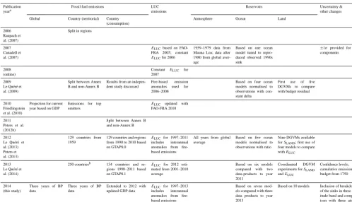
Table 3.Main methodological changes in the global carbon budget since first publication. Unless specified below, the methodology was identical to that described in the current paper. Furthermore, methodological changes introduced in one year are kept for the following years unless noted. Empty cells mean there were no methodological changes introduced that year.
Publication
yeara
Fossil fuel emissions LUC
emissions
Reservoirs Uncertainty &
other changes
Global Country (territorial) Country
(consumption)
Atmosphere Ocean Land
2006 Raupach et al. (2007)
Split in regions
2007 Canadell et al. (2007)
ELUCbased on
FAO-FRA 2005; constant
ELUCfor 2006
1959–1979 data from Mauna Loa; data after 1980 from global aver-age
Based on one ocean model tuned to repro-duced observed 1990s sink
±1σ provided for all
components
2008 (online)
Constant ELUC for
2007
2009 Le Quéré et al. (2009)
Split between Annex B and non-Annex B
Results from an indepen-dent study discussed
Fire-based emission
anomalies used for
2006–2008
Based on four ocean models normalised to observations with con-stant delta
First use of five
DGVMs to compare
with budget residual
2010 Friedlingstein et al. (2010)
Projection for current year based on GDP
Emissions for top
emitters
ELUC updated with
FAO-FRA 2010
2011 Peters et al. (2012b)
Split between Annex B and non-Annex B
2012 Le Quéré et al. (2013) Peters et al. (2013)
129 countries from 1959
129 countries and regions from 1990 to 2010 based on GTAP8.0
ELUCfor 1997–2011
includes interannual
anomalies from
fire-based emissions
All years from global average
Based on five ocean models normalised to observations with ratio
Nine DGVMs available forSLAND; first use of four models to compare
withELUC
2013 Le Quéré et al. (2014)
250 countriesb 134 countries and
re-gions 1990–2011 based on GTAP8.1
ELUCfor 2012
esti-mated from 2001–2010 average
Based on six models
compared with two
data-products to year 2011
Coordinated DGVM
experiments forSLAND
andELUC
Confidence levels; cumulative emissions; budget from 1750
2014 (this study)
Three years of BP data
Three years of BP data
Extended to 2012 with updated GDP data
ELUCfor 1997–2013
includes interannual
anomalies from
fire-based emissions
Based on seven mod-els compared with three data products to year 2013
Based on 10 models Inclusion of breakdown
of the sinks in three lat-itude band and compar-ison with three atmo-spheric inversions
aThe naming convention of the budgets has changed. Up to and including 2010, the budget year (Carbon Budget 2010) represented the latest year of the data. From 2012, the budget year (Carbon Budget 2012) refers to the initial publication year. bThe CDIAC database has about 250 countries, but we show data for about 216 countries since we aggregate and disaggregate some countries to be consistent with current country definitions (see Sect. 2.1.1 for more details).
of flared or vented fuel. For emission years 2011–2013, flar-ing is assumed constant from 2010 (emission year) UN-based data. The basic data on gas flaring report atmospheric losses during petroleum production and processing that have large uncertainty and do not distinguish between gas that is flared as CO2or vented as CH4. Fugitive emissions of CH4from the
so-called upstream sector (e.g. coal mining and natural gas distribution) are not included in the accounts of CO2
emis-sions except to the extent that they are captured in the UN energy data and counted as gas “flared or lost”.
The published CDIAC data set has 250 countries and re-gions included. This expanded list includes countries/rere-gions that no longer exist, such as the USSR and East Pakistan. For the budget, we reduce the list to 216 countries by real-locating emissions to the currently defined territories. This involved both aggregation and disaggregation, and does not change global emissions. Examples of aggregation include merging East and West Germany to the currently defined Germany. Examples of disaggregation include reallocating the emissions from the former USSR to the resulting inde-pendent countries. For disaggregation, we use the emission shares when the current territory first appeared. For the most recent years, 2011–2013, the BP statistics are more aggre-gated, but we retain the detail of CDIAC by applying the
growth rates of each aggregated region in the BP data set to its constituent individual countries in CDIAC.
Estimates of CO2emissions show that the global total of
emissions is not equal to the sum of emissions from all coun-tries. This is largely attributable to emissions that occur in international territory, in particular the combustion of fuels used in international shipping and aviation (bunker fuels), where the emissions are included in the global totals but are not attributed to individual countries. In practice, the emis-sions from international bunker fuels are calculated based on where the fuels were loaded, but they are not included with national emissions estimates. Other differences occur because globally the sum of imports in all countries is not equal to the sum of exports and because of differing treat-ment of oxidation of non-fuel uses of hydrocarbons (e.g. as solvents, lubricants, feedstocks), and changes in stock (An-dres et al., 2012).
The uncertainty in the annual fossil fuel and cement emis-sions for the globe has been estimated at±5 % (scaled down from the published±10 % at±2σto the use of±1σ bounds reported here; Andres et al., 2012). This is consistent with a more detailed recent analysis of uncertainty of±8.4 % at
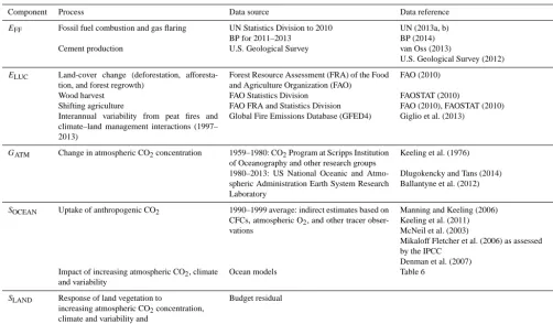
Table 4.Data sources used to compute each component of the global carbon budget.
Component Process Data source Data reference
EFF Fossil fuel combustion and gas flaring UN Statistics Division to 2010 UN (2013a, b)
BP for 2011–2013 BP (2014)
Cement production U.S. Geological Survey van Oss (2013)
U.S. Geological Survey (2012) ELUC Land-cover change (deforestation,
afforesta-tion, and forest regrowth)
Forest Resource Assessment (FRA) of the Food and Agriculture Organization (FAO)
FAO (2010)
Wood harvest FAO Statistics Division FAOSTAT (2010)
Shifting agriculture FAO FRA and Statistics Division FAO (2010), FAOSTAT (2010) Interannual variability from peat fires and
climate–land management interactions (1997– 2013)
Global Fire Emissions Database (GFED4) Giglio et al. (2013)
GATM Change in atmospheric CO2concentration 1959–1980: CO2Program at Scripps Institution of Oceanography and other research groups
Keeling et al. (1976) 1980–2013: US National Oceanic and
Atmo-spheric Administration Earth System Research Laboratory
Dlugokencky and Tans (2014) Ballantyne et al. (2012)
SOCEAN Uptake of anthropogenic CO2 1990–1999 average: indirect estimates based on CFCs, atmospheric O2, and other tracer obser-vations
Manning and Keeling (2006) Keeling et al. (2011) McNeil et al. (2003)
Mikaloff Fletcher et al. (2006) as assessed by the IPCC
Denman et al. (2007) Impact of increasing atmospheric CO2, climate
and variability
Ocean models Table 6
SLAND Response of land vegetation to
increasing atmospheric CO2concentration, climate and variability and
other environmental changes
Budget residual
and heat contents of fuels, and the combustion efficiency. While in the budget we consider a fixed uncertainty of±5 % for all years, in reality the uncertainty, as a percentage of the emissions, is growing with time because of the larger share of global emissions from non-Annex B countries (emerging economies and developing countries) with less precise sta-tistical systems (Marland et al., 2009). For example, the un-certainty in Chinese emissions has been estimated at around
±10 % (for±1σ; Gregg et al., 2008). Generally, emissions from mature economies with good statistical bases have an uncertainty of only a few percent (Marland, 2008). Further research is needed before we can quantify the time evolu-tion of the uncertainty, and its temporal error correlaevolu-tion structure. We note that, even if they are presented as 1σ es-timates, uncertainties of emissions are likely to be mainly country-specific systematic errors related to underlying bi-ases of energy statistics and to the accounting method used by each country. We assign a medium confidence to the re-sults presented here because they are based on indirect esti-mates of emissions using energy data (Durant et al., 2010). There is only limited and indirect evidence for emissions, although there is a high agreement among the available es-timates within the given uncertainty (Andres et al., 2012, 2014), and emission estimates are consistent with a range of other observations (Ciais et al., 2013), even though their
re-gional and national partitioning is more uncertain (Francey et al., 2013).
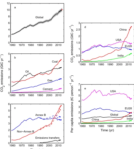
Davis and Caldeira, 2010) provide additional information on territorial-based emissions that can be used to under-stand emission drivers (Hertwich and Peters, 2009), quantify emission (virtual) transfers by the trade of products between countries (Peters et al., 2011b), and potentially design more effective and efficient climate policy (Peters and Hertwich, 2008).
We estimate consumption-based emissions by enumerat-ing the global supply chain usenumerat-ing a global model of the eco-nomic relationships between ecoeco-nomic sectors within and between every country (Andrew and Peters, 2013; Peters et al., 2011a). Due to availability of the input data, detailed es-timates are made for the years 1997, 2001, 2004, and 2007 (using the methodology of Peters et al., 2011b) using eco-nomic and trade data from the Global Trade and Analysis Project version 8.1 (GTAP; Narayanan et al., 2013). The re-sults cover 57 sectors and 134 countries and regions. The results are extended into an annual time series from 1990 to the latest year of the fossil fuel emissions or GDP data (2012 in this budget), using GDP data by expenditure in current ex-change rate of US dollars (USD; from the UN National Ac-counts Main Aggregates database; UN, 2014) and time series of trade data from GTAP (based on the methodology in Pe-ters et al., 2011b).
The consumption-based emission inventories in this car-bon budget incorporate several improvements over previous versions (Le Quéré et al., 2013; Peters et al., 2011b, 2012b). The detailed estimates for 2004 and 2007 and time series ap-proximation from 1990 to 2012 are based on an updated ver-sion of the GTAP database (Narayanan et al., 2013). We es-timate the sector level CO2emissions using our own
calcula-tions based on the GTAP data and methodology, include flar-ing and cement emissions from CDIAC, and then scale the national totals (excluding bunker fuels) to match the CDIAC estimates from the most recent carbon budget. We do not in-clude international transportation in our estimates of national totals, but we do include them in the global total. The time se-ries of trade data provided by GTAP covers the period 1995– 2009 and our methodology uses the trade shares as this data set. For the period 1990–1994 we assume the trade shares of 1995, while for 2010 and 2011 we assume the trade shares of 2008 since 2009 was heavily affected by the global financial crisis. We identified errors in the trade shares of Taiwan in 2008 and 2009, so its trade shares for 2008–2010 are based on the 2007 trade shares.
We do not provide an uncertainty estimate for these emis-sions, but based on model comparisons and sensitivity analy-sis, they are unlikely to be larger than for the territorial emis-sion estimates (Peters et al., 2012a). Uncertainty is expected to increase for more detailed results and decrease with ag-gregation (Peters et al., 2011b; e.g. the results for Annex B countries will be more accurate than the sector results for an individual country).
The consumption-based emissions attribution method con-siders the CO2emitted to the atmosphere in the production
of products, but not the trade in fossil fuels (coal, oil, gas). It is also possible to account for the carbon trade in fossil fuels (Davis et al., 2011), but we do not present those data here. Peters et al. (2012a) additionally considered trade in biomass.
The consumption data do not modify the global average terms in Eq. (1), but they are relevant to the anthropogenic carbon cycle as they reflect the trade-driven movement of emissions across the Earth’s surface in response to human activities. Furthermore, if national and international climate policies continue to develop in an unharmonised way, then the trends reflected in these data will need to be accommo-dated by those developing policies.
2.1.3 Growth rate in emissions
We report the annual growth rate in emissions for adjacent years (in percent per year) by calculating the difference be-tween the 2 years and then comparing to the emissions in the first year:
E
FF(t0+1)−EFF(t0)
EFF(t
0)
×% yr−1. This is the simplest method to characterise a 1-year growth compared to the pre-vious year and is widely used. We apply a leap-year adjust-ment to ensure valid interpretations of annual growth rates. This affects the growth rate by about 0.3 % yr−1 (3651 ) and causes growth rates to go up approximately 0.3 % if the first year is a leap year and down 0.3 % if the second year is a leap year.
The relative growth rate of EFF over time periods of
greater than 1 year can be re-written using its logarithm equivalent as follows:
1 EFF
dEFF
dt =
d(lnEFF)
dt . (2)
Here we calculate relative growth rates in emissions for multi-year periods (e.g. a decade) by fitting a linear trend to ln(EFF) in Eq. (2), reported in percent per year. We fit
the logarithm ofEFFrather than EFF directly because this
method ensures that computed growth rates satisfy Eq. (6). This method differs from previous papers (Canadell et al., 2007; Le Quéré et al., 2009; Raupach et al., 2007) that com-puted the fit toEFFand divided by averageEFFdirectly, but
the difference is very small (<0.05 %) in the case ofEFF.
GDP (USD yr−1) and the fossil fuel carbon intensity of the
economy (IFF; GtC USD−1) as follows:
EFF=GDP×IFF. (3)
Such product-rule decomposition identities imply that the relative growth rates of the multiplied quantities are additive. Taking a time derivative of Eq. (3) gives
dEFF
dt =
d(GDP×IFF)
dt , (4)
and, applying the rules of calculus, dEFF
dt = dGDP
dt ×IFF+GDP× dIFF
dt ; (5)
finally, dividing Eq. (5) by Eq. (3) gives 1
EFF
dEFF
dt = 1 GDP
dGDP dt +
1 IFF
dIFF
dt , (6)
where the left-hand term is the relative growth rate ofEFF,
and the right-hand terms are the relative growth rates of GDP andIFF, respectively, which can simply be added linearly to
give overall growth rate. The growth rates are reported in per-cent by multiplying each term by 100. As preliminary esti-mates of annual change in GDP are made well before the end of a calendar year, making assumptions on the growth rate of IFF allows us to make projections of the annual change in
CO2emissions well before the end of a calendar year.
2.2 CO2emissions from land use, land-use change, and forestry (ELUC)
LUC emissions reported in the 2014 carbon budget (ELUC)
include CO2 fluxes from deforestation, afforestation,
log-ging (forest degradation and harvest activity), shifting culti-vation (cycle of cutting forest for agriculture and then aban-doning), and regrowth of forests following wood harvest or abandonment of agriculture. Only some land management activities (Table 5) are included in our LUC emissions es-timates (e.g. emissions or sinks related to management and management changes in established pasture and croplands are not included). Some of these activities lead to emissions of CO2to the atmosphere, while others lead to CO2sinks. ELUC is the net sum of all anthropogenic activities
consid-ered. Our annual estimate for 1959–2010 is from a book-keeping method (Sect. 2.2.1) primarily based on net forest area change and biomass data from the Forest Resource As-sessment (FRA) of the Food and Agriculture Organization (FAO), which is only available at intervals of 5 years and ends in 2010 (Houghton et al., 2012). Interannual variabil-ity in emissions due to deforestation and degradation have been coarsely estimated from satellite-based fire activity in tropical forest areas (Sect. 2.2.2; Giglio et al., 2013; van der Werf et al., 2010). The bookkeeping method is used to quantify theELUCover the time period of the available data,
and the satellite-based deforestation fire information to incor-porate interannual variability (ELUCflux annual anomalies)
from tropical deforestation fires. The satellite-based defor-estation and degradation fire emissions estimates are avail-able for years 1997–2013. We calculate the global annual anomaly in deforestation and degradation fire emissions in tropical forest regions for each year, compared to the 1997– 2010 period, and add this annual flux anomaly to theELUC
estimated using the bookkeeping method that is available up to 2010 only and assumed constant at the 2010 value during the period 2011–2013. We thus assume that all land manage-ment activities apart from deforestation and degradation do not vary significantly on a year-to-year basis. Other sources of interannual variability (e.g. the impact of climate variabil-ity on regrowth fluxes) are accounted for inSLAND. In
ad-dition, we use results from dynamic global vegetation mod-els (see Sect. 2.2.3 and Table 6) that calculate net LUC CO2
emissions in response to land-cover-change reconstructions prescribed to each model in order to help quantify the uncer-tainty inELUCand to explore the consistency of our
under-standing. The three methods are described below, and differ-ences are discussed in Sect. 3.2.
2.2.1 Bookkeeping method
LUC CO2emissions are calculated by a bookkeeping method
approach (Houghton, 2003) that keeps track of the carbon stored in vegetation and soils before deforestation or other land-use change, and the changes in forest age classes, or cohorts, of disturbed lands after land-use change including possible forest regrowth after deforestation. It tracks the CO2
emitted to the atmosphere immediately during deforestation, and over time due to the follow-up decay of soil and vegeta-tion carbon in different pools, including wood product pools after logging and deforestation. It also tracks the regrowth of vegetation and associated build-up of soil carbon pools after LUC. It considers transitions between forests, pastures, and cropland; shifting cultivation; degradation of forests where a fraction of the trees is removed; abandonment of agricultural land; and forest management such as wood harvest and, in the USA, fire management. In addition to tracking logging debris on the forest floor, the bookkeeping method tracks the fate of carbon contained in harvested wood products that is eventually emitted back to the atmosphere as CO2, although
a detailed treatment of the lifetime in each product pool is not performed (Earles et al., 2012). Harvested wood products are partitioned into three pools with different turnover times. All fuel wood is assumed burned in the year of harvest (1.0 yr−1).
Pulp and paper products are oxidised at a rate of 0.1 yr−1, timber is assumed to be oxidised at a rate of 0.01 yr−1, and elemental carbon decays at 0.001 yr−1. The general assump-tions about partitioning wood products among these pools are based on national harvest data (Houghton, 2003).
Table 5.Comparison of the processes included in theELUCof the global carbon budget and the DGVMs. See Table 6 for model references.
All models include deforestation and forest regrowth after abandonment of agriculture (or from afforestation activities on agricultural land).
Bookk
eeping
CABLE CLM4.5BGC ISAM JULES LPJ-GUESS LPJ LPX ORCHIDEE VEGAS VISIT
Wood harvest and for-est degradationa
yes yes yes yes no no no no no yes yesb
Shifting cultivation yes no yes no no no no no noc nod yes
Cropland harvest yes yes yes no no yes no yes yes yes yes
Peat fires no no yes no no no no no no no no
Fire simulation and/or suppression
for US only no yes no no yes yes yes no yes yes
Climate and variability no yes yes yes yes yes yes yes yes yes yes CO2fertilisation no yes yes yes yes yes yes yes yes yes yes
Carbon–nitrogen interactions, including N deposition
no yes yes yes no no no yes no no no
aRefers to the routine harvest of established managed forests rather than pools of harvested products.bWood stems are harvested according to
the land-use data.cModels only used to calculateSLAND.dModel only used to compareELUC+SLANDto atmospheric inversions (Fig. 6).
Assessment of the FAO, which provides statistics on forest-cover change and management at intervals of 5 years (FAO, 2010). The data are based on countries’ self-reporting, some of which includes satellite data in more recent assessments (Table 4). Changes in land cover other than forest are based on annual, national changes in cropland and pasture areas reported by the FAO Statistics Division (FAOSTAT, 2010). LUC country data are aggregated by regions. The carbon stocks on land (biomass and soils), and their response func-tions subsequent to LUC, are based on FAO data averages per land-cover type, biome, and region. Similar results were obtained using forest biomass carbon density based on satel-lite data (Baccini et al., 2012). The bookkeeping method does not include land ecosystems’ transient response to changes in climate, atmospheric CO2, and other environmental factors,
but the growth/decay curves are based on contemporary data that will implicitly reflect the effects of CO2and climate at
that time. Results from the bookkeeping method are available from 1850 to 2010.
2.2.2 Fire-based method
LUC-associated CO2 emissions calculated from
satellite-based fire activity in tropical forest areas (van der Werf et al., 2010) provide information on emissions due to tropical deforestation and degradation that are complementary to the bookkeeping approach. They do not provide a direct estimate of ELUC as they do not include non-combustion processes
such as respiration, wood harvest, wood products, and forest regrowth. Legacy emissions such as decomposition from on-ground debris and soils are not included in this method either. However, fire estimates provide some insight into the
year-to-year variations in the sub-component of the totalELUCflux
that result from immediate CO2emissions during
deforesta-tion caused, for example, by the interacdeforesta-tions between climate and human activity (e.g. there is more burning and clearing of forests in dry years) that are not represented by other meth-ods. The “deforestation fire emissions” assume an important role of fire in removing biomass in the deforestation process, and thus can be used to infer gross instantaneous CO2
emis-sions from deforestation using satellite-derived data on fire activity in regions with active deforestation. The method re-quires information on the fraction of total area burned as-sociated with deforestation versus other types of fires, and this information can be merged with information on biomass stocks and the fraction of the biomass lost in a deforestation fire to estimate CO2emissions. The satellite-based
deforesta-tion fire emissions are limited to the tropics, where fires re-sult mainly from human activities. Tropical deforestation is the largest and most variable single contributor toELUC.
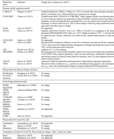
Table 6.References for the process models and data products included in Figs. 6–8.
Model/data name
Reference Change from Le Quéré et al. (2013)
Dynamic global vegetation models
CABLE2.0 Zhang et al. (2013) Updated model from CABLE1.4 (Wang et al., 2011) to include full carbon, nitrogen, and phos-phorus cycle (Wang et al., 2010) and land cover and land-cover change.
CLM4.5BGCa Oleson et al. (2013) Updated model from CLM4.0CN to CLM4.5BGC. Major changes include revised photosynthe-sis, slower turnover times for decomposition of litter and SOM, vertically resolved soil biogeo-chemistry, revised soil denitrification and nitrification, new fire model, and revised frozen-soil hydrology. As shown in Koven et al. (2013), these changes collectively bring model into better agreement with 20th century C budget.
ISAM Jain et al. (2013)b Not applicable
JULESc Clark et al. (2011)d Updated model from JULESv1 (Cox et al., 2000) to JULESv3.2 as configured in the latest generation ESM-HadGEM2-ES (Collins et al., 2011). Higher resolution (1.875×1.25) and with an improved snow scheme, multi-pool soil carbon model, updated representation of land-use change.
LPJ-GUESS Smith et al. (2001) Not applicable
LPJe Sitch et al. (2003) Decreased LPJ wood harvest efficiency so that 50 % of biomass was removed off-site compared to 85 % used in the 2012 budget. Residue management of managed grasslands increased so that 100 % of harvested grass enters litter pool.
LPX Stocker et al. (2013a) Addition of C–N cycle coupling.
ORCHIDEE Krinner et al. (2005) Revised parameters values for photosynthetic capacity for boreal forests (following assimilation of FLUXNET data), updated parameters values for stem allocation, maintenance respiration and biomass export for tropical forests (based on literature), and CO2down-regulation process added to photosynthesis.
VEGAS Zeng et al. (2005)f Improved wetland and permafrost parameterisations, high-latitude temperature dependence VISIT Kato et al. (2013)g Wood harvest flux is added toE
LUC, and the loss of additional sink capacity is also included in theELUCdue to the methodological change of using coordinated DGVM experiments. Data products for land-use-change emissions
Bookkeeping Houghton et al. (2012) No change Fire-based
emissions
van der Werf et al. (2010) No change
Ocean biogeochemistry models
NEMO-PlankTOM5
Buitenhuis et al. (2010)h No change
NEMO-PISCES (IPSL)i
Aumont and Bopp (2006) No change
CCSM-BEC Doney et al. (2009) No change
MICOM-HAMOCC
Assmann et al. (2010)j No change
MPIOM-HAMOCC
Ilyina et al. (2013) No change
NEMO-PISCES (CNRM)
Séférian et al. (2013)k Not applicable
CSIRO Oke et al. (2013) Not applicable Data products for ocean CO2sink
Landschützer Landschützer et al. (2014) Not applicable Park Park et al. (2010)l No change Rödenbeck Rödenbeck et al. (2014)m No change
Atmospheric inversions for total CO2fluxes (land-use change+land+ocean CO2sinks) Peters Peters et al. (2010) Not applicable
Rödenbeck Rödenbeck et al. (2003) Not applicable MACCn Chevallier et al. (2005) Not applicable
aCommunity Land Model 4.5.bSee also El-Masri et al. (2013).cJoint UK Land Environment Simulator.dSee also Best et al. (2011)eLund–Potsdam–Jena.fOnly used for total land
(ELUC+SLAND)flux calculation of multi-model mean.gSee also Ito and Inatomi (2012).hWith no nutrient restoring below the mixed layer depth.iReferred to as LSCE in previous carbon
budgets.jWith updates to the physical model as described in Tjiputra et al. (2013).kFurther information (e.g. physical evaluation) for CNRM model can be found in Danabasoglu et
al. (2014).lUsing winds from Atlas et al. (2011).mUpdated version “s81_v3.6gcp”.nThe MACC v13.1 CO2inversion system, initially described by Chevallier et al. (2005), relies on the
decay functions compared to the bookkeeping method, and does not include historical emissions or regrowth from land-use change prior to the availability of satellite data. Compar-ing coincident CO emissions and their atmospheric fate with satellite-derived CO concentrations allows for some valida-tion of this approach (e.g. van der Werf et al., 2008). Re-sults from the fire-based method to estimate LUC emissions anomalies added to the bookkeeping meanELUCestimate are
available from 1997 to 2013. Our combination of LUC CO2
emissions where the variability of annual CO2deforestation
emissions is diagnosed from fires assumes that year-to-year variability is dominated by variability in deforestation.
2.2.3 Dynamic global vegetation models (DGVMs) LUC CO2 emissions have been estimated using an
ensem-ble of seven DGVMs. New model experiments up to year 2013 have been coordinated by the project “Trends and drivers of the regional-scale sources and sinks of carbon dioxide” (TRENDY; http://dgvm.ceh.ac.uk/node/9). We use only models that have estimated LUC CO2 emissions and
the terrestrial residual sink following the TRENDY protocol (see Sect. 2.5.2), thus providing better consistency in the as-sessment of the causes of carbon fluxes on land. Models use their latest configurations, summarised in Tables 5 and 6.
The DGVMs were forced with historical changes in land-cover distribution, climate, atmospheric CO2concentration,
and N deposition. As further described below, each histor-ical DGVM simulation was repeated with a time-invariant pre-industrial land-cover distribution, allowing for estima-tion of, by difference with the first simulaestima-tion, the dynamic evolution of biomass and soil carbon pools in response to prescribed land-cover change. All DGVMs represent defor-estation and (to some extent) regrowth, the most important components ofELUC, but they do not represent all processes
resulting directly from human activities on land (Table 5). DGVMs represent processes of vegetation growth and mor-tality, as well as decomposition of dead organic matter asso-ciated with natural cycles, and include the vegetation and soil carbon response to increasing atmospheric CO2levels and to
climate variability and change. In addition, four models ex-plicitly simulate the coupling of C and N cycles and account for atmospheric N deposition (Table 5). The DGVMs are in-dependent of the other budget terms except for their use of atmospheric CO2concentration to calculate the fertilisation
effect of CO2on primary production.
The DGVMs used a consistent land-use-change data set (Hurtt et al., 2011), which provided annual, half-degree, frac-tional data on cropland, pasture, and primary and secondary vegetation, as well as all underlying transitions between land-use states, including wood harvest and shifting cultivation. This data set used the HYDE (Klein Goldewijk et al., 2011) spatially gridded maps of cropland, pasture, and ice/water fractions of each grid cell as an input. The HYDE data are based on annual FAO statistics of change in agricultural area
(FAOSTAT, 2010). For the years 2011, 2012, and 2013, the HYDE data set was extrapolated by country for pastures and cropland separately based on the trend in agricultural area over the previous 5 years. The HYDE data set is independent of the data set used in the bookkeeping method (Houghton, 2003, and updates), which is based primarily on forest area change statistics (FAO, 2010). Although the Hurtt land-use-change data set indicates whether land-use land-use-changes occur on forested or non-forested land, typically only the changes in agricultural areas are used by the models and are im-plemented differently within each model (e.g. an increased cropland fraction in a grid cell can be at the expense of ei-ther grassland or forest, the latter resulting in deforestation; land-cover fractions of the non-agricultural land differ be-tween models). Thus the DGVM forest area and forest area change over time is not consistent with the Forest Resource Assessment of the FAO forest area data used for the book-keeping model to calculateELUC. Similarly, model-specific
assumptions are applied to convert deforested biomass or de-forested area, and other forest product pools, into carbon in some models (Table 5).
The DGVM model runs were forced by either 6-hourly CRU-NCEP or monthly temperature, precipitation, and cloud cover fields (transformed into incoming surface radi-ation) based on observations and provided on a 0.5◦×0.5◦ grid and updated to 2013 (CRU TS3.22; Harris et al., 2014). The forcing data include both gridded observations of cli-mate and global atmospheric CO2, which change over time
(Dlugokencky and Tans, 2014), and N deposition (as used in 4 models, Table 5; Lamarque et al., 2010).ELUCis diagnosed
in each model by the difference between a model simula-tion with prescribed historical land-cover change and a sim-ulation with constant, pre-industrial land-cover distribution. Both simulations were driven by changing atmospheric CO2,
climate, and, in some models, N deposition over the period 1860–2013. Using the difference between these two DGVM simulations to diagnoseELUCis not consistent with the
defi-nition ofELUCin the bookkeeping method (Gasser and Ciais,
2013; Pongratz et al., 2014). The DGVM approach to di-agnose land-use-change CO2 emissions would be expected
to produce systematically higherELUC emissions than the
bookkeeping approach if all the parameters of the two ap-proaches were the same (which is not the case). Here, given the different input data of DGVMs and the bookkeeping ap-proach, this systematic difference cannot be quantified.
2.2.4 Uncertainty assessment forELUC
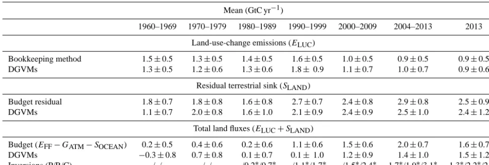
Table 7.Comparison of results from the bookkeeping method and budget residuals with results from the DGVMs and inverse estimates for the periods 1960–1969, 1970–1979, 1980–1989, 1990–1999, 2000–2009, last decade, and last year available. All values are in GtC yr−1. The DGVM uncertainties represents±1σof results from the nine individual models; for the inverse models all three results are given where available.
Mean (GtC yr−1)
1960–1969 1970–1979 1980–1989 1990–1999 2000–2009 2004–2013 2013
Land-use-change emissions (ELUC)
Bookkeeping method 1.5±0.5 1.3±0.5 1.4±0.5 1.6±0.5 1.0±0.5 0.9±0.5 0.9±0.5
DGVMs 1.3±0.5 1.2±0.6 1.3±0.6 1.8±0.9 1.1±0.7 1.0±0.7 0.9±0.6
Residual terrestrial sink (SLAND)
Budget residual 1.8±0.7 1.8±0.8 1.6±0.8 2.7±0.7 2.4±0.8 2.9±0.8 2.5±0.9
DGVMs 1.1±0.7 2.0±0.8 1.6±1.0 2.1±0.9 2.4±0.9 2.5±1.0 2.4±1.2
Total land fluxes (ELUC+SLAND)
Budget (EFF−GATM−SOCEAN) 0.2±0.5 0.4±0.6 0.2±0.6 1.1±0.6 1.5±0.6 2.0±0.7 1.6±0.7
DGVMs −0.3±0.8 0.7±0.8 0.1±0.7 0.1±1.0 1.2±0.9 1.4±1.0 1.5±1.2
Inversions (P/R/C) –/–/– –/–/– –/0.2∗/0.7∗ –/1.1∗/1.7∗ –/1.5∗/2.4∗ 1.7∗/1.9∗/3.1∗ 1.3∗/2.2∗/2.7∗
∗Estimates are not corrected for the influence of river fluxes, which would reduce the fluxes by 0.45 GtC yr−1when neglecting the anthropogenic influence on land (Sect. 7.2.2).
Note: letters identify each of the three inversions (P for Peters, R for Rödenbeck, and C for Chevallier).
The uncertainties in the annual ELUC estimates are
ex-amined using the standard deviation across models, which ranged from 0.3 to 1.1 GtC yr−1, with an average of
0.7 GtC yr−1from 1959 to 2013 (Table 7). The mean of the multi-modelELUCestimates is the same as the mean of the
bookkeeping estimate from the budget (Eq. 1) at 1.3 GtC for 1959 to 2010. The multi-model mean and bookkeeping method differ by less than 0.5 GtC yr−1 over 90 % of the time. Based on this comparison, we assess that an uncer-tainty of ±0.5 GtC yr−1 provides a semi-quantitative mea-sure of uncertainty for annual emissions and reflects our best value judgment that there is at least 68 % chance (±1σ) that the true LUC emission lies within the given range, for the range of processes considered here. This is consistent with the uncertainty analysis of Houghton et al. (2012), which partly reflects improvements in data on forest area change using data, and partly more complete understanding and rep-resentation of processes in models. The uncertainties in the decadal mean estimates from the DGVM ensemble are likely correlated between decades, and thus we apply the annual uncertainty as a measure of the decadal uncertainty. The cor-relations between decades come from (1) common biases in system boundaries (e.g. not counting forest degradation in some models); (2) common definition for the calculation of ELUC from the difference of simulations with and without
LUC (a source of bias vs. the unknown truth); and (3) com-mon and uncertain land-cover-change input data which also cause a bias (though if a different input data set is used each decade, decadal fluxes from DGVMs may be partly decorre-lated); and (4) model structural errors (e.g. systematic errors in biomass stocks). In addition, errors arising from uncertain DGVM parameter values would be random, but they are not
accounted for in this study, since no DGVM provided an en-semble of runs with perturbed parameters.
Prior to 1959, the uncertainty inELUCis taken as±33 %,
which is the ratio of uncertainty to mean from the 1960s (Table 7), the first decade available. This ratio is consistent with the mean standard deviation of DGMVs’ LUC emis-sions over 1870–1958 (0.41 GtC) over the multi-model mean (0.94 GtC).
2.3 Atmospheric CO2growth rate (GATM) Global atmospheric CO2growth rate estimates
The atmospheric CO2growth rate is provided by the US
Na-tional Oceanic and Atmospheric Administration Earth Sys-tem Research Laboratory (NOAA/ESRL; Dlugokencky and Tans, 2014), which is updated from Ballantyne et al. (2012). For the 1959–1980 period, the global growth rate is based on measurements of atmospheric CO2 concentration averaged
from the Mauna Loa and South Pole stations, as observed by the CO2 Program at Scripps Institution of
Oceanogra-phy (Keeling et al., 1976). For the 1980–2012 time period, the global growth rate is based on the average of multi-ple stations selected from the marine boundary layer sites with well-mixed background air (Ballantyne et al., 2012), after fitting each station with a smoothed curve as a func-tion of time, and averaging by latitude band (Masarie and Tans, 1995). The annual growth rate is estimated by Dlu-gokencky and Tans (2014) from atmospheric CO2
mul-tiplying by a factor of 2.120 GtC ppm−1(Prather et al., 2012)
for consistency with the other components.
The uncertainty around the annual growth rate based on the multiple stations data set ranges between 0.11 and 0.72 GtC yr−1, with a mean of 0.60 GtC yr−1for 1959–1980 and 0.19 GtC yr−1for 1980–2013, when a larger set of sta-tions were available (Dlugokencky and Tans, 2014). It is based on the number of available stations, and thus takes into account both the measurement errors and data gaps at each station. This uncertainty is larger than the uncertainty of±0.1 GtC yr−1reported for decadal mean growth rate by the IPCC because errors in annual growth rate are strongly anti-correlated in consecutive years, leading to smaller er-rors for longer timescales. The decadal change is com-puted from the difference in concentration 10 years apart based on a measurement error of 0.35 ppm. This error is based on offsets between NOAA/ESRL measurements and those of the World Meteorological Organization World Data Center for Greenhouse Gases (NOAA/ESRL, 2014) for the start and end points (the decadal change uncertainty is the q
2(0.35 ppm)2(10 yr)−1assuming that each yearly mea-surement error is independent). This uncertainty is also used in Table 8.
The contribution of anthropogenic CO and CH4 is
ne-glected from the global carbon budget (see Sect. 2.7.1). We assign a high confidence to the annual estimates ofGATM
be-cause they are based on direct measurements from multiple and consistent instruments and stations distributed around the world (Ballantyne et al., 2012).
In order to estimate the total carbon accumulated in the at-mosphere since 1750 or 1870, we use an atmospheric CO2
concentration of 277±3 or 288±3 ppm, respectively, based on a cubic spline fit to ice core data (Joos and Spahni, 2008). The uncertainty of ±3 ppm (converted to±1σ) is taken di-rectly from the IPCC’s assessment (Ciais et al., 2013). Typi-cal uncertainties in the atmospheric growth rate from ice core data are ±1–1.5 GtC decade−1 as evaluated from the Law Dome data (Etheridge et al., 1996) for individual 20-year in-tervals over the period from 1870 to 1960 (Bruno and Joos, 1997).
2.4 Ocean CO2sink
Estimates of the global ocean CO2sink are based on a
com-bination of a mean CO2 sink estimate for the 1990s from
observations and a trend and variability in the ocean CO2
sink for 1959–2013 from seven global ocean biogeochem-istry models. We use three observation-based estimated of SOCEANavailable for the recent decade(s) to provide a
quali-tative assessment of confidence in the reported results.
2.4.1 Observation-based estimates
A mean ocean CO2sink of 2.2±0.4 GtC yr−1for the 1990s
was estimated by the IPCC (Denman et al., 2007) based
on indirect observations and their spread: ocean–land CO2
sink partitioning from observed atmospheric O2/N2
con-centration trends (Keeling et al., 2011; Manning and Keel-ing, 2006), an oceanic inversion method constrained by ocean biogeochemistry data (Mikaloff Fletcher et al., 2006), and a method based on penetration time scale for CFCs (McNeil et al., 2003). This is comparable with the sink of 2.0±0.5 GtC yr−1 estimated by Khatiwala et al. (2013) for the 1990s, and with the sink of 1.9 to 2.5 estimated from a range of methods for the period 1990–2009 (Wan-ninkhof et al., 2013), with uncertainties ranging from±0.3 to ±0.7 GtC yr−1. The most direct way to estimate the observation-based ocean sink is from the product of (sea– airpCO2 difference)×(gas transfer coefficient). Estimates
based on sea–airpCO2are fully consistent with indirect
ob-servations (Zeng et al., 2005), but their uncertainty is larger mainly due to difficulty in capturing complex turbulent pro-cesses in the gas transfer coefficient (Sweeney et al., 2007).
Two of the three observation-based estimates computed the interannual variability in the ocean CO2 sink using
in-terpolated measurements of surface ocean fugacity of CO2
(pCO2 corrected for the non-ideal behaviour of the gas;
Pfeil et al., 2013). The measurements were from the Surface Ocean CO2Atlas (SOCAT v2; Bakker et al., 2014), which
contains data to the end of 2011. This was extended with 2.4 million additional measurements from 2012 and 2013 from all basins (see data attribution table in Appendix A), submitted to SOCAT but not yet fully quality-controlled fol-lowing standard SOCAT procedures. Revisions and correc-tions to measurements from before 2012 were also included where they were available. All new data were subjected to an automated quality control system to detect and remove the most obvious errors (e.g. incorrect reporting of meta-data such as position, wrong units, clearly unrealistic meta-data). The combined SOCAT v2 and preliminary 2012–2013 data were implemented in an inversion method (Rödenbeck et al., 2013) and a combined self-organising map and feed-forward neural network (Landschützer et al., 2014). The observation-based estimates were corrected to remove a background (not part of the anthropogenic ocean flux) ocean source of CO2
to the atmosphere of 0.45 GtC yr−1 from river input to the ocean (Jacobson et al., 2007) so as to make them compara-ble toSOCEAN, which only represents the annual uptake of
anthropogenic CO2by the ocean.
We also compare the results with those of Park et al. (2010) based on regional correlations between surface temperature andpCO2, changes in surface temperature observed by
satel-lite, and wind speed estimates also from satellite data for 1990–2009 (Atlas et al., 2011). The product of Park et al. (2010) provides a data-based assessment of the interan-nual variability combined with a model-based assessment of the trend and mean inSOCEAN. Several other data-based