www.geosci-model-dev.net/8/957/2015/ doi:10.5194/gmd-8-957-2015
© Author(s) 2015. CC Attribution 3.0 License.
Twelve-month, 12 km resolution North American WRF-Chem v3.4
air quality simulation: performance evaluation
C. W. Tessum1, J. D. Hill2, and J. D. Marshall1
1Department of Civil, Environmental, and Geo- Engineering, University of Minnesota, Minneapolis, Minnesota, USA 2Department of Bioproducts and Biosystems Engineering, University of Minnesota, St. Paul, Minnesota, USA Correspondence to: J. D. Marshall ([email protected])
Received: 3 November 2014 – Published in Geosci. Model Dev. Discuss.: 2 December 2014 Revised: 24 February 2015 – Accepted: 9 March 2015 – Published: 7 April 2015
Abstract. We present results from and evaluate the perfor-mance of a 12-month, 12 km horizontal resolution year 2005 air pollution simulation for the contiguous United States using the WRF-Chem (Weather Research and Forecasting with Chemistry) meteorology and chemical transport model (CTM). We employ the 2005 US National Emissions In-ventory, the Regional Atmospheric Chemistry Mechanism (RACM), and the Modal Aerosol Dynamics Model for Eu-rope (MADE) with a volatility basis set (VBS) secondary aerosol module. Overall, model performance is compara-ble to contemporary modeling efforts used for regulatory and health-effects analysis, with an annual average day-time ozone (O3) mean fractional bias (MFB) of 12 % and an annual average fine particulate matter (PM2.5) MFB of −1 %. WRF-Chem, as configured here, tends to overpredict total PM2.5 at some high concentration locations and gen-erally overpredicts average 24 h O3concentrations. Perfor-mance is better at predicting daytime-average and daily peak O3 concentrations, which are more relevant for regulatory and health effects analyses relative to annual average val-ues. Predictive performance for PM2.5subspecies is mixed: the model overpredicts particulate sulfate (MFB=36 %), un-derpredicts particulate nitrate (MFB= −110 %) and organic carbon (MFB= −29 %), and relatively accurately predicts particulate ammonium (MFB=3 %) and elemental carbon (MFB=3 %), so that the accuracy in total PM2.5predictions is to some extent a function of offsetting over- and underpre-dictions of PM2.5subspecies. Model predictive performance for PM2.5and its subspecies is in general worse in winter and in the western US than in other seasons and regions, suggest-ing spatial and temporal opportunities for future WRF-Chem model development and evaluation.
1 Introduction
Epidemiological studies have established the importance of health effects from acute and chronic exposure to fine par-ticulate matter (PM2.5) and ground-level ozone (O3) (Jerrett et al., 2009; Krewski et al., 2009; Pope III and Dockery, 2006). The accuracy of health-impact predictions for future air pollutant emissions (e.g., Tessum et al., 2012, 2014) de-pends in part on the performance of air quality models over long timescales and in all seasons. Accurate health-impact predictions often depend on model simulations that cover large geographic areas such as the contiguous US, so as to capture the full impacts of the long-range transport of pollu-tants (Levy et al., 2003). Whereas chemical transport model (CTM) simulations for a full year for the contiguous US often use 36 km horizontal grids (e.g., Tesche et al., 2006; Yahya et al., 2014), increasing horizontal grid resolution to 12 km can result in the more accurate prediction of pollutant con-centrations (Fountoukis et al., 2013) and population expo-sure. However, increasing horizontal resolution from 36 to 12 km in a CTM typically results in a∼27 times increase in computational intensity (number of grid cells increases nine-fold; number of time steps increases threefold).
sec-ond study (not peer reviewed), the US EPA (2012) describes model evaluation for PM2.5 concentrations for year 2007, also for the contiguous US and using CMAQ. Our study con-tributes to this literature by evaluating a different model with different parameterizations over a different time period. We also provide greater investigation regarding how model per-formance varies in space, in time, and by chemical species.
We employ and evaluate the performance of WRF-Chem (the Weather Research and Forecasting model with Chem-istry) (Grell et al., 2005) for year 2005 for a North Ameri-can domain. WRF-Chem is functionally similar to CMAQ, but differs from the version used by Appel et al. (2012) in that WRF-Chem predicts meteorological quantities and air pollution concentrations simultaneously, allowing meteorol-ogy quantities to be updated more frequently as the model is running and allowing representation of interactions between meteorology and air pollution. WRF-Chem users can follow a simplified modeling workflow that does not require run-ning a separate meteorological model. Combined meteorol-ogy/chemical transport models can be more computationally demanding than standalone CTMs; however, for the domain and settings used here, meteorological modeling accounts for only∼10 % of the total computational expense.
Table A1 summarizes spatial and temporal aspects of re-cent chemical transport model evaluation efforts, with a fo-cus on WRF-Chem evaluations in the US. WRF-Chem per-formance in predicting air quality observations has been ex-tensively quantified for simulations of individual regions of the US, with simulation periods of several weeks or months (Ahmadov et al., 2012; Chuang et al., 2011; Fast et al., 2006; Grell et al., 2005; McKeen et al., 2007; Misenis and Zhang, 2010; Zhang et al., 2010, 2012). One study evalu-ated WRF-Chem performance for a full year for the contigu-ous US with a 36 km grid (Yahya et al., 2014). We present here WRF-Chem results from a full year, 12 km resolution simulation for the contiguous US, evaluate the performance of the model compared to ambient measurements, and com-pare WRF-Chem performance to published goals and criteria (Boylan and Russell, 2006) and to recent CMAQ results for a similar simulation (Appel et al., 2012).
2 Methods 2.1 Model setup
We run the WRF-Chem model version 3.4 using a 12 km res-olution grid with 444 rows, 336 columns, and 28 vertical lay-ers. The modeling domain (see Fig. 1) covers the contiguous US, southern Canada, and northern Mexico. Previous studies (e.g., Appel et al., 2012; Yahya et al., 2014) have used 34 vertical layers; our choice of 28 vertical layers represents a tradeoff between vertical grid resolution and computational expense.
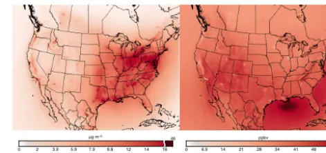
0 2 3.9 5.9 7.9 9.8 12 14 16 46 μg m−3
0 6.9 14 21 28 34 41 48 55 57 ppbv
(a) Total PM2.5 (b) Average O3
Figure 1. Modeled annual average ground level (a) PM2.5 and (b) O3concentrations. For ease of viewing, the color scales con-tain a break at the 99th percentile of concentrations.
Within WRF-Chem, we use the Regional Atmospheric Chemistry Mechanism (RACM) (Stockwell et al., 1997) for gas-phase reactions and the Modal Aerosol Dynamics for Eu-rope (MADE) (Ackermann et al., 1998) module for aerosol chemistry and physics. RACM and MADE were selected be-cause of their relatively modest computational expense; at the time of this study, alternatives to RACM/MADE are im-practical for large-scale simulations such as ours. We use the volatility basis set (VBS) (Ahmadov et al., 2012) to simu-late formation and evaporation of secondary organic aerosol (SOA). The VBS approach differs from other SOA param-eterizations in that it assumes that primary organic aerosol (POA) is semi-volatile. Meteorology options are set as rec-ommended by the WRF user manual (Wang et al., 2012) and the WRF-Chem user manual (Peckham et al., 2012) for situ-ations similar to those studied here. Table 1 summarizes the model options and inputs used. See supporting information for additional details.
We use results from the MOZART global chemical trans-port model (Emmons et al., 2010) as processed by the MOZBC file format converter (available at: http://web3.acd. ucar.edu/wrf-chem) to provide initial and boundary condi-tions for chemical species. Because the MOZBC bound-ary conditions for unclassified PM2.5are unrealistic for the southeastern edges of the modeling domain – their use re-sults in substantial PM2.5 overpredictions in the southeast-ern US – we set all initial and boundary concentrations to zero for unclassified PM2.5. As in Ahmadov et al. (2012), owing to uncertainty in secondary organic aerosol (SOA) concentrations over the open ocean, we assume that initial and boundary concentrations of SOA are zero. Data from the National Centers for Environmental Prediction (NCEP) Eta model (UCAR, 2005) provide meteorological inputs, bound-ary conditions, and, for the four-dimensional data assimila-tion (FDDA) employed here, observaassimila-tional “nudging” val-ues.
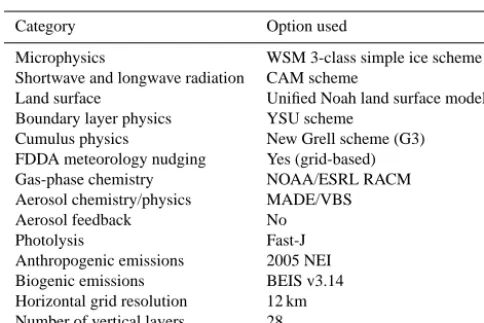
Table 1. Selected WRF-Chem v3.4 settings and parameters em-ployed in this study.
Category Option used
Microphysics WSM 3-class simple ice scheme
Shortwave and longwave radiation CAM scheme
Land surface Unified Noah land surface model
Boundary layer physics YSU scheme
Cumulus physics New Grell scheme (G3)
FDDA meteorology nudging Yes (grid-based)
Gas-phase chemistry NOAA/ESRL RACM
Aerosol chemistry/physics MADE/VBS
Aerosol feedback No
Photolysis Fast-J
Anthropogenic emissions 2005 NEI
Biogenic emissions BEIS v3.14
Horizontal grid resolution 12 km
Number of vertical layers 28
in Mexico. We use the model evaluation version of the NEI, which also includes hourly Continuous Emission Monitor-ing System (CEMS) data for electricity-generatMonitor-ing units, hourly wildfire data, and biogenic emissions from the BEIS model (Biogenic Emission Inventory System; Schwede et al., 2005), version 3.14.
We prepare pollutant emissions at 12 km spatial resolu-tion using the Sparse Matrix Operating Kernel Emissions (SMOKE) program (Houyoux and Vukovich, 1999), ver-sion 2.6, as bundled with the NEI data (available at: http: //www.epa.gov/ttn/chief/emch/index.html), then we convert the emission files output by SMOKE to WRF-Chem format and apply a plume-rise algorithm (ASME, 1973, as cited in Seinfeld and Pandis, 2006) to estimate the mixing height of elevated emission sources and wildfires. Source code for the file format conversion and plume-rise program is available at https://bitbucket.org/ctessum/emcnv.
We simulate atmospheric pollutant concentrations for the period from 1 January through to 31 December 2005. We choose the year 2005 because at the time this study was per-formed it was the most recent year for which emissions data were available. For logistical expediency, we separate the year into eight independent model runs, each approximately 1.5 months in length plus a discarded 5-day model spin-up period. We run the simulations on a high-performance com-puting system consisting of 2.8 GHz Intel Xeon X5560 “Ne-halem EP” processors with a 40 Gbit QDR InfiniBand (IB) interconnect and a Lustre parallel file system. Using 768 pro-cessors, each 1.5-month model run takes∼19 h to complete (∼13 processor years for each annual model run).
2.2 Comparison with observations
We compare WRF-Chem wind speed, air temperature, rel-ative humidity, and precipitation predictions to data from the US Environmental Protection Agency (EPA) Clean Air Status and Trends Network (CASTNET) observations. We
compare modeled ground-level concentrations of total PM2.5 to EPA Air Quality System (AQS) observations (US EPA, 2005) using 24 h average data (EPA parameter code 88101) and using the less extensive hourly measurement network (EPA parameter code 88502), which allows us to compare modeled vs. measured diurnal profiles. We compare WRF-Chem predictions of O3 to measurements from the AQS (EPA parameter code 44201) and CASTNET networks. We compare the predictions of PM2.5subspecies to observation data from the EPA’s Chemical Speciation Network (CSN) (US EPA, 2005) (formally called Speciation Trends Network (STN)) for organic carbon (OC, parameter code 88305), el-emental carbon (EC, code 88307), particulate sulfate (SO4, code 88403), particulate nitrate (NO3, code 88306), and particulate ammonium (NH4, code 88301). We additionally compare predictions to data from the Interagency Monitor-ing of Protected Visual Environments (IMPROVE) network (University of California Davis, 1995) for particulate OC (code 88320), EC (code 88321), sulfur (code 88169), and NO3(code 88306); and to CASTNET observations for par-ticulate SO4, NH4, and NO3. WRF-Chem outputs organic aerosol (OA) concentrations, but methods for measuring or-ganic aerosol only quantify OC. OC comprises a variable fraction of OA, but it is common to assume an OA : OC ra-tio of 1.4 (Aiken et al., 2008). Therefore, we divide WRF-Chem OA predictions by a factor of 1.4 for comparison with OC measurements. Finally, we compare WRF-Chem predic-tions of gas-phase sulfur dioxide (SO2) and nitrogen dioxide (NO2) to AQS observations. We remove from consideration those stations with≥25 % missing data relative to the num-ber of scheduled measurements during the simulation period. The fractions of excluded data for each type of comparison are in the Supplement.
WRF-Chem, as configured here, outputs instantaneous concentrations at the start of each hour, whereas the obser-vation data are reported as hourly or daily averages. WRF-Chem calculates grid-cell-average concentrations, whereas observations generally represent concentrations at specific locations.
We compare measured and modeled values pair-wise at each time of measurement in the grid cell containing each measurement station. The 24 h average measurements are compared to the average of the modeled (hourly instanta-neous) values within the same period. Comparisons are only made with observations that occur within the first (nearest to ground) model layer (height:∼50–60 m). The source code for the program used to extract and pair model and mea-surement data is available at https://bitbucket.org/ctessum/ aqmcompare.
2.3 Aggregation of results
spatial approaches. First, we use four regional subdomains: Midwest, Northeast, South, and West (basis: US Census re-gions (US Census Bureau, 2013); see Fig. 2). Second, we evaluate urban vs. rural (i.e., not urban) locations, also as de-fined by the US Census (US Census Bureau, 2014). CSN monitors tend to be placed in urban areas (85 % of 186 monitors are urban), whereas IMPROVE monitors tend to be placed in protected rural areas (10 % of 122 monitors are urban). All 67 monitors in the CASTNET network are in rural locations. We also split the analysis into four sea-sons: winter (January–March), spring (April–June), summer (July–September), and fall (October–December). Employing these time periods allows us to compare against previously published results (Appel et al., 2012).
2.4 Performance metrics
After matching all measured values with their corresponding modeled values, and averaging modeled and measured val-ues across the appropriate time period, we calculate metrics shown in Eqs. (1)–(8):
MB=1
n n X
i=1
(Mi−Oi), (1)
ME=1
n n X
i=1
|Mi−Oi|, (2)
NMB= n P
i=1
(Mi−Oi)
n P
i=1 Oi
×100 %, (3)
NME= n P
i=1
|Mi−Oi|
n P
i=1 Oi
×100 %, (4)
MFB=1
n n X
i=1
2(Mi−Oi) Mi+Oi
×100 %, (5)
MFE=1
n n X
i=1
2|Mi−Oi| Mi+Oi
×100 %, (6)
MR=1
n n X
i=1 Mi Oi , (7) RMSE= v u u u t n P
i=1
(Mi−Oi)2
n , (8)
whereicorresponds to one ofnmeasurement locations,M andO are time-averaged modeled and observed values, re-spectively, MB is mean bias, ME is mean error, NMB is nor-malized mean bias, NME is nornor-malized mean error, MFB is mean fractional bias, MFE is mean fractional error, MR is model ratio, and RMSE is root-mean-square error. We
ad-(a) Total PM2.5 (b) Daytime O3 AQS AQS Hourly PM2.5 CASTNET
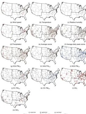
Figure 2. AQS, AQS hourly, and CASTNET monitor locations and annual average fractional bias for (a) total PM2.5and (b) daytime average O3 concentrations. Corresponding information for other pollutants and variables is in Fig. A1.
ditionally calculate the slope (S), intercept (I), and squared Pearson correlation coefficient (R2) of a linear regression be-tween modeled and measured values.
Each metric provides a useful and distinct evaluation of model performance. In general, metrics with “bias” in the name evaluate the accuracy of the model, whereas metrics with “error” in the name incorporate both precision and ac-curacy. Metrics that are in normalized or fractional form tend to emphasize errors where measured and observed values are relatively small, whereas non-normalized metrics tend to em-phasize errors where measured and observed values are rela-tively large. We mainly focus here on MFB andR2to evalu-ate performance as they facilitevalu-ate direct comparisons among pollutants. Results for all combinations of time periods, mea-surement networks, spatial subdomains, and metrics are in the Supplement.
For O3, we calculate model performance via three model–measurement comparisons: (1) annual averages; (2) daytime-only (08:00–20:00 LT) annual averages, as in Appel et al. (2012); and (3) annual averages of daily peak concentrations, to match the epidemiological findings in Jer-rett et al. (2009).
Figure 3. Annual average modeled and measured ground-level (a– d) meteorological variables and (e–o) pollutant concentrations. Col-ored lines show linear least-squares fits of the data for the measure-ment networks with corresponding colors. Grey lines show model to measurement ratios of 2:1, 1:1, and 1:2. Annual average per-formance statistics are listed to the right of each plot; acronyms are defined in the methods section.
3 Results
Figure 1 shows modeled annual average concentrations of PM2.5 and O3, where the edges of the maps represent the edges of the modeling domain. An animated version of Fig. 1 showing pollutant concentration as a function of time is available in the Supplement. Maps of additional pollutants, as well as monthly, weekly, and diurnal maps and profiles of population-weighted average concentrations, are also avail-able in the Supplement. Modeled O3concentrations over wa-ter in the Gulf of Mexico and along the Atlantic coast tend to be higher than concentrations over the adjacent land areas. As only areas over water appear to be affected (as Fig. 2a shows, O3overpredictions along the Gulf of Mexico and At-lantic coasts are not greater than overpredictions further in-land), this over-water anomaly in the Gulf of Mexico should
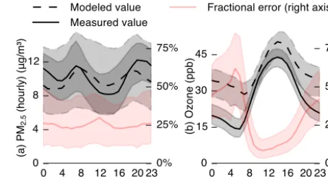
0 4 8 12 16 20 23
0 4 8 12 0% 25% 50% 75%
0 4 8 12 16 20 23
0 15 30 45 0% 25% 50% 75% (a ) P M2 .5 ( h o u rl y) ( μ g /m ³)
Hour of day
(b) Ozone (ppb)
Modeled value Measured value
Fractional error (right axis)
Figure 4. Median values (lines) and interquartile ranges (shaded areas) of annual average modeled values, observed values, and frac-tional error by hour of day for (a) PM2.5and (b) O3.
not adversely impact estimates of population-weighted con-centrations.
Figure 2 shows monitor locations for total PM2.5and for O3, as well as annual average fractional bias (MFB) values at each monitor. Results in Fig. 2a (PM2.5) display high spatial variability, with no obvious spatial patterns in model perfor-mance; large overpredictions are sometimes adjacent to large underpredictions (e.g., in southern Louisiana and Florida). WRF-Chem generally overpredicts daytime O3 concentra-tions relative to observaconcentra-tions (Fig. 2b). Monitor locaconcentra-tions for meteorological variables, PM2.5 subspecies, and other gas phase species are in Fig. A1.
3.1 Meteorological performance
Figure 3 contains scatterplots comparing annual average ob-served and predicted values for meteorological variables and pollutant concentrations. The model tends to overpredict near-ground wind speed (Fig. 3a) and precipitation (Fig. 3d) relative to observations, whereas temperature (Fig. 3b) and relative humidity (Fig. 3c) predictions agree well with obser-vations. Figures A2–A5 in Appendix A disaggregate model performance for meteorological variables by region (region boundaries are shown in Fig. 2) and by season; meteoro-logical performance is relatively consistent among seasons and regions. Model–measurement comparisons provide im-portant evidence on model performance but might overes-timate model robustness for meteorological parameters be-cause FDDA “nudges” model meteorological estimates to-ward observed values.
3.2 PM2.5and O3performance
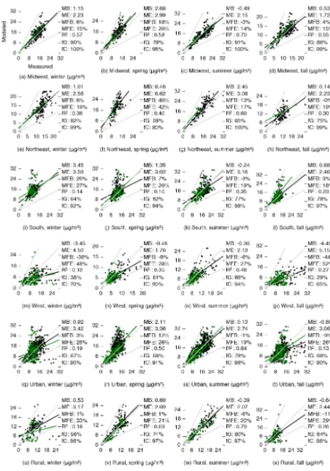
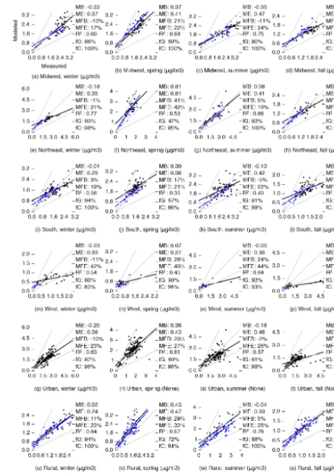
aver-Figure 5. Comparison of measured and modeled PM2.5 concentra-tions disaggregated by season and region. Region boundaries are shown in Fig. 2.
age concentrations (Fig. 3f) than for daily peak (Fig. 3g) and daytime average (Fig. 3f) concentrations.
Figure 4 shows the median and interquartile range for modeled and measured PM2.5and O3concentrations by hour of day (measurements of PM2.5subspecies are only available as 24 h averages). For PM2.5, the model generally agrees with measurements, although on average it underpredicts concen-trations at night and overpredicts during the day (Fig. 4a). For O3, on average the model overpredicts for all times of day but with a much lower fractional error during the day than during the night. For both pollutants, the model accurately captures the timing of diurnal trends, including the afternoon peak for O3 and the morning and evening peaks for PM2.5. As a result, when comparing the three averaging-time met-rics for O3, we observe better model performance for the an-nual average of daily peak concentration (MFB=11 %) and of average daytime concentration (MFB=12 %) than for the overall annual average (MFB=23 %). For O3, the first two metrics may offer greater relevance than the third. For exam-ple, the annual average of daily peak concentrations is more strongly correlated with health effects than are annual
aver-Figure 6. Comparison of measured and modeled annual average of daytime O3concentrations disaggregated by season and region. Region boundaries are shown in Fig. 2.
age concentrations (Jerrett et al., 2009); and, for comparisons to the 8 h peak concentration National Ambient Air Quality Standard (NAAQS), model performance is more important during daytime than at night.
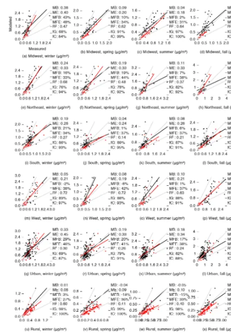
Figure 7. Comparison of modeled and measured particulate SO4 concentrations, disaggregated by region and season.
CTMs and may be attributable to difficulty in reproducing the strongly stable meteorological conditions that are responsi-ble for high winter PM concentrations (Solazzo et al., 2012). Annual average PM2.5 predictive performance in the West (AQSR2: 0.45 (summer), 0.13 (winter)) is worse than perfor-mance in the Northeast (AQSR2: 0.70 (summer), 0.37 (win-ter)). In the Northeast, performance is better in the summer (R2=0.69) than in other seasons (R2=0.30–0.40). Taken together, these findings suggest that there is an opportunity for future model development for PM2.5 to focus on win-ter or full-year simulations rather than summer-only simula-tions, and on the western US or the full contiguous US rather than just the Northeast.
3.3 PM2.5subspecies performance
Figure 3i–m illustrates model performance for annual aver-age concentrations of PM2.5component species. In all cases, >65 % of locations meet performance criteria for at least one of the three observation networks.
The model overpredicts particulate SO4 (CSN MFB=34 %, IMPROVE MFB=40 %, CASTNET
Figure 8. Comparison of modeled and measured particulate NH4 concentrations, disaggregated by region and season.
MFB=36 %) (Fig. 3i) and SO2 (MFB=51 %) (Fig. 3n). This finding (overprediction of total sulfur) agrees with prior research for multiple CTMs (McKeen et al., 2007). Partic-ulate SO4 prediction performance does not vary much by region; as with total PM2.5, performance is worse in winter (CSN MFB=59 %) than in summer (CSN MFB=10. %) (Fig. 7).
WRF-Chem as configured here performs well in predict-ing observed particulate NH4 concentrations, with 99 % of locations meeting performance criteria (Fig. 3j). Similar to total PM2.5, performance for particulate NH4is worst in the urban areas in the West region (Fig. 8), where a number of monitors report relatively high measured concentrations but modeled concentrations are relatively low.
Figure 9. Comparison of modeled and measured particulate NO3 concentrations, disaggregated by region and season.
opportunity for future development and evaluation of mod-els for particulate NO3 prediction to focus on seasons and regions other than summer in the Northeast. Predictions of gas-phase NO2 (Fig. 3o) agree relatively well with obser-vations (MFB=4 %) but, as with other species, the model tends to overpredict NO2concentrations in areas where mea-sured concentrations are relatively high. This effect is espe-cially prominent in the West and in urban areas (Fig. A9).
Model–measurement agreement for EC concentrations is relatively good (Fig. 3l), with 96 % of monitor locations meeting performance criteria. As with other comparisons, for EC the model tends to overpredict concentrations for moni-tors with relatively high concentrations, especially in urban areas (Fig. 10).
Model predictions of OC concentrations (Fig. 3m) are bi-ased low compared to CSN (MFB= −55 %) but agree rela-tively well with IMPROVE (MFB=15 %). Mean bias val-ues given here are within the range of valval-ues reported by a previous publication using the VBS SOA formation mech-anism (Ahmadov et al., 2012). As shown in Fig. 11, the dif-ferences in model–measurement agreement between the two networks do not appear to be dependent on urban vs. rural
Figure 10. Comparison of modeled and measured particulate EC concentrations, disaggregated by region and season.
monitor location. Instead, they may reflect between-network differences in sampling or analysis; different analysis tech-niques are known to produce widely varying OC concentra-tions (Cavalli et al., 2010).
3.4 Comparison with other studies
Table 2 compares performance of WRF-Chem as configured here to that of the CMAQ model in a similar modeling effort by Appel et al. (2012). In this table, CMAQ as configured by Appel et al. (2012) in most cases predicts O3 observa-tions with greater accuracy and precision than does WRF-Chem as configured here, while WRF-WRF-Chem in most cases does a better job predicting PM2.5. However, given the many differences in physical and chemical parameterizations and input data (including a difference in simulation year), the ob-served differences may or may not be generalizable. Instead, our conclusion from Table 2 is that the models are generally comparable in performance.
resolu-Table 2. WRF-Chem and CMAQ seasonal O3and PM2.5prediction performance.
Daytimea PM2.5
average O3(ppb) (µg m−3)
WRF-Chem CMAQb WRF-Chem CMAQb
Winter MB 3.5 −3.5 0.8 3.4
Spring MB 1.5 −1.8 2.0 2.0
Summer MB 9.2 4.4 0.0 −0.6
Fall MB 5.2 2.6 −0.9 4.0
Winter ME 5.5 9.0 3.1 6.0
Spring ME 4.6 9.3 3.3 4.5
Summer ME 10.1 11.0 2.6 4.4
Fall ME 6.2 8.8 2.7 5.6
Winter NMB 12 % −13 % 6 % 30 %
Spring NMB 3 % −4 % 17 % 19 %
Summer NMB 21 % 10. % 0 % −5 %
Fall NMB 19 % 8 % −7 % 36 %
Winter NME 19 % 35 % 25 % 53 %
Spring NME 10 % 29 % 28 % 42 %
Summer NME 23 % 24 % 18 % 31 %
Fall NME 23 % 28 % 23 % 52 %
aDaytime is defined as 08:00–20:00 LT.bAdapted from Appel et al. (2012) Tables 1 and 2.
tion spatial grid. NME results from the simulation performed here are lower (i.e., better) than those reported by Yahya et al. (2014) for most pollutants and measurement networks, but NMB results are more mixed. As horizontal grid resolu-tion, input data, and model parameters all differ between the two studies, we are not able to determine the cause of the differences in results.
4 Discussion
We simulated and evaluated PM2.5 and O3 based on 12-month (year 2005) WRF-Chem modeling for the United States. The spatial and temporal extent investigated, and the horizontal spatial resolution (12 km) employed, are nearly unprecedented; to our knowledge, only one prior peer-reviewed CTM evaluation has used a comparable extent and resolution (Appel et al., 2012). We find that WRF-Chem per-formance as configured here is generally comparable to other models used in regulatory and health impact assessment sit-uations in that model performance is similar to that reported by Appel et al. (2012) and, in most cases, meets the criteria for air quality model performance suggested by Boylan and Russel (2006).
There is potential for further improvement in model accu-racy, especially for these cases: PM2.5concentrations in win-ter and in the weswin-tern US, ground-level O3at night and in the summer, and particulate nitrate. The good agreement in to-tal PM2.5predictions and observations in some cases reflects offsetting over- and underpredictions, including by species (Fig. 3) and time of day (Fig. 4a). Performance in predicting concentrations of PM2.5 and its subspecies tends to be the
Figure 11. Comparison of modeled and measured particulate OC concentrations, disaggregated by region and season.
worst in winter and in the western US. Overall, WRF-Chem as configured here meets the performance criteria described above for total PM2.5concentrations at 94 % of monitor lo-cations.
Appendix A
Figure A2. Comparison of modeled and measured wind speed, dis-aggregated by region and season.
Figure A4. Comparison of modeled and measured relative humid-ity, disaggregated by region and season.
Figure A6. Comparison of modeled and measured annual average O3concentrations, disaggregated by region and season.
Figure A8. Comparison of modeled and measured SO2 concentra-tions, disaggregated by region and season.
Table A1. Temporal and spatial aspects of recent model evaluations, focusing on WRF-Chem and North America.
Author and year Model used Time period Spatial extent Horizontal spatial resolution
Ahmadov et al. (2012) WRF-Chem Aug–Sep 2006 Contiguous US (evaluation performed for eastern US)
60 and 20 km
Appel et al. (2012) CMAQ Full year, 2006 Contiguous US and Europe
12 km
Chuang et al. (2011) WRF-Chem May–Sep 2009 Southeastern US 12 km Fast et al. (2006) WRF-Chem Late Aug 2000 City of Houston 1.3 km
Grell et al. (2005) WRF-Chem Jul–Aug 2002 Eastern US 27 km
McKeen et al. (2007) WRF-Chem, CHRONOS, AURAMS, STEM, CMAQ/ETA
Jul–Aug 2004 Northeastern US 12, 21, 27, and 42 km
Misenis and Zhang (2010) WRF-Chem Late Aug 2000 Eastern Texas 4 and 12 km Tesche et al. (2006) CMAQ,
CAMx
Full year, 2002 Contiguous US 12 km eastern US, 36 km contiguous US Yahya et al. (2014) WRF-Chem Full year, 2006 Contiguous US 36 km
Zhang et al. (2010) WRF-Chem Late Aug 2010 Eastern Texas 12 km
Zhang et al. (2012) WRF-Chem Jul 2001 Contiguous US 36 km
Table A2. WRF-Chem annual average predictive performance by pollutant in Yahya et al. (2014) and in the current study.
Variable Network MB NMB NME
Yahya et Current Yahya et Current Yahya et Current al. (2014) study al. (2014) study al. (2014) study
Daily peak O3(ppb) CASTNET −8.6 3.9 −18 % 9 % 24 % 12 %
AQS −0.3 5.5 −5 % 13 % 9 % 15 %
Daytime average O3(ppb) CASTNET −5.6 3.5 −13 % 9 % 22 % 11 %
AQS −1.7 4.9 −4 % 13 % 24 % 16 %
SO2(ppb) AQS −0.6 5.1 −18 % 130 % 87 % 150 %
NO2(ppb) AQS 1.7 1.6 17 % 12 % 73 % 34 %
Total PM2.5(µg m−3) CSN 0.0 0.4 0 % 3 % 45 % 18 %
SO4PM2.5(µg m−3) IMPROVE 0.5 0.9 35 % 40 % 66 % 42 %
CSN 0.9 1.6 32 % 41 % 59 % 42 %
CASTNET 0.9 1.3 34 % 38 % 55 % 38 %
NH4PM2.5(µg m−3) CSN 0.1 0.0 10. % −2 % 53 % 16 %
CASTNET 0.3 0.1 30. % 7 % 50. % 16 %
NO3PM2.5(µg m−3) IMPROVE −0.1 −0.5 −14 % −69 % 85 % 69 %
CSN −0.6 −1.3 −38 % −72 % 75 % 72 %
CASTNET −0.1 −0.7 −15 % −65 % 83 % 65 %
EC PM2.5(µg m−3) IMPROVE 0.0 0.0 15 % −9 % 67 % 31 %
CSN 0.4 0.2 54 % 25 % 90. % 43 %
Supporting information
Supplement includes WRF-Chem configuration settings (ASCII format); maps showing spatial patterns in pollutant concentrations by annual average, month of year, day of week, and hour of day (PDF format); model–measurement comparison statistics (XLSX format); and monitor-specific paired model and measurement data (JSON ASCII format). A video showing spatially and temporally explicit O3 and PM2.5concentrations is at http://youtu.be/4bpQXBAUVwE. The Supplement related to this article is available online at doi:10.5194/gmd-8-957-2015-supplement.
Acknowledgements. We acknowledge the University of Minnesota
Institute on the Environment Initiative for Renewable Energy and the Environment grant no. Rl-0026-09 and the US Department of Energy award no. DE-EE0004397 for funding, the Minnesota Supercomputing Institute and the Department of Energy National Center for Computational Sciences award no. DD-ATM007 for computational resources, Steven Roste for assistance with model– measurement comparison, and John Michalakes for assistance with WRF-Chem performance tuning.
Edited by: V. Grewe
References
Ackermann, I. J., Hass, H., Memmesheimer, M., Ebel, A., Binkowski, F. S., and Shankar, U.: Modal Aerosol Dynamics Model for Europe: development and first applications, Atmos. Environ., 32, 2981–2999, 1998.
Ahmadov, R., McKeen, S. A., Robinson, A. L., Bahreini, R., Middlebrook, A. M., de Gouw, J. A., Meagher, J., Hsie, E.-Y., Edgerton, E., Shaw, S., and Trainer, M.: A volatility basis set model for summertime secondary organic aerosols over the eastern United States in 2006, J. Geophys. Res., 117, D06301, doi:10.1029/2011JD016831, 2012.
Aiken, A. C., DeCarlo, P. F., Kroll, J. H., Worsnop, D. R., Huff-man, J. A., Docherty, K. S., Ulbrich, I. M., Mohr, C., Kim-mel, J. R., Sueper, D., Sun, Y., Zhang, Q., Trimborn, A., North-way, M., Ziemann, P. J., Canagaratna, M. R., Onasch, T. B., Al-farra, M. R., Prevot, A. S. H., Dommen, J., Duplissy, J., Met-zger, A., Baltensperger, U., and Jimenez, J. L.: O/C and OM/OC ratios of primary, secondary, and ambient organic aerosols with high-resolution time-of-flight aerosol mass spectrometry, Envi-ron. Sci. Technol., 42, 4478–4485, 2008.
ASME (American Society of Mechanical Engineers): Recom-mended Guide for the Prediction of the Dispersion of Airborne Effluents, 2nd Edn., ASME, New York, NY, 1973.
Appel, K. W., Chemel, C., Roselle, S. J., Francis, X. V., Hu, R.-M., Sokhi, R. S., Rao, S. T., and Galmarini, S.: Examination of the Community Multiscale Air Quality (CMAQ) model perfor-mance over the North American and European domains, Atmos. Environ., 53, 142–155, 2012.
Boylan, J. W. and Russell, A. G.: PM and light extinction model performance metrics, goals, and criteria for three-dimensional air quality models, Atmos. Environ., 40, 4946–4959, 2006. Cavalli, F., Viana, M., Yttri, K. E., Genberg, J., and Putaud, J.-P.:
Toward a standardised thermal-optical protocol for measuring atmospheric organic and elemental carbon: the EUSAAR proto-col, Atmos. Meas. Tech., 3, 79–89, doi:10.5194/amt-3-79-2010, 2010.
Chuang, M.-T., Zhang, Y., and Kang, D.: Application of WRF/Chem-MADRID for real-time air quality forecasting over the southeastern United States, Atmos. Environ., 45, 6241–6250, 2011.
Emmons, L. K., Walters, S., Hess, P. G., Lamarque, J.-F., Pfister, G. G., Fillmore, D., Granier, C., Guenther, A., Kinnison, D., Laepple, T., Orlando, J., Tie, X., Tyndall, G., Wiedinmyer, C., Baughcum, S. L., and Kloster, S.: Description and evaluation of the Model for Ozone and Related chemical Tracers, version 4 (MOZART-4), Geosci. Model Dev., 3, 43–67, doi:10.5194/gmd-3-43-2010, 2010.
Fast, J. D., Gustafson Jr., W. I., Easter, R. C., Zaveri, R. A., Barnard, J. C., Chapman, E. G., Grell, G. A., and Peck-ham, S. E.: Evolution of ozone, particulates, and aerosol direct radiative forcing in the vicinity of Houston using a fully coupled meteorology-chemistry-aerosol model, J. Geophys. Res., 111, D21305, doi:10.1029/2005JD006721, 2006.
Foley, K. M., Roselle, S. J., Appel, K. W., Bhave, P. V., Pleim, J. E., Otte, T. L., Mathur, R., Sarwar, G., Young, J. O., Gilliam, R. C., Nolte, C. G., Kelly, J. T., Gilliland, A. B., and Bash, J. O.: Incremental testing of the Community Multiscale Air Quality (CMAQ) modeling system version 4.7, Geosci. Model Dev., 3, 205–226, doi:10.5194/gmd-3-205-2010, 2010.
Fountoukis, C., Koraj, D., Denier van der Gon, H. A. C., Charalam-pidis, P. E., Pilinis, C., and Pandis, S. N.: Impact of grid resolu-tion on the predicted fine PM by a regional 3-D chemical trans-port model, Atmos. Environ., 68, 24–32, 2013.
Galmarini, S., Rao, S. T., and Steyn, D. G.: AQMEII: an interna-tional initiative for the evaluation of regional-scale air quality models – Phase 1 preface, Atmos. Environ., 53, 1–3, 2012. Grell, G. A., Peckham, S. E., Schmitz, R., McKeen, S. A., Frost, G.,
Skamarock, W. C., and Eder, B.: Fully coupled “online” chem-istry within the WRF model, Atmos. Environ., 39, 6957–6975, 2005.
Houyoux, M. R. and Vukovich, J. M.: Updates to the Sparse Ma-trix Operator Kernel Emissions (SMOKE) modeling system and integration with Models-3, in: Proceedings of the Emission In-ventory: Regional Strategies for the Future, Air and Waste Man-agement Association, Raleigh, NC, 26–28 October 1999, 1999. Jerrett, M., Burnett, R. T., Pope III, C. A., Ito, K., Thurston, G.,
Krewski, D., Shi, Y., Calle, E., and Thun, M.: Long-term ozone exposure and mortality, New Engl. J. Med., 360, 1085–1095, 2009.
Levy, J. I., Wilson, A. M., Evans, J. S., and Spengler, J. D.: Estima-tion of primary and secondary particulate matter intake fracEstima-tions for power plants in Georgia, Environ. Sci. Technol., 37, 5528– 5536, 2003.
McKeen, S., Chung, S. H., Wilczak, J., Grell, G., Djalalova, I., Peckham, S., Gong, W., Bouchet, V., Moffet, R., Tang, Y., Carmichael, G. R., Mathur, R., and Yu, S.: Evaluation of sev-eral PM2.5 forecast models using data collected during the ICARTT/NEAQS 2004 field study, J. Geophys. Res., 112, D10S20, doi:10.1029/2006JD007608, 2007.
Misenis, C. and Zhang, Y.: An examination of sensitivity of WRF/Chem predictions to physical parameterizations, horizon-tal grid spacing, and nesting options, Atmos. Res., 97, 315–334, 2010.
Peckham, S. E., Grell, G. A., McKeen, S. A., Ahmadov, R., Barth, M., Pfister, G., Wiedinmyer, C., Fast, J. D., Gustafson, W. I., Ghan, S. J., Zaveri, R., Easter, R. C., Barnard, J., Chapman, E., Hewson, M., Schmitz, R., Salz-mann, M., Beck, V., and Freitas, S. R.: WRF/Chem Version 3.4 User’s Guide, available at: http://ruc.noaa.gov/wrf/WG11 (last access: 18 December 2012), 2012.
Pope III, C. A. and Dockery, D. W.: Health effects of fine particulate air pollution: lines that connect, J. Air Waste Manage., 56, 709– 742, 2006.
Schwede, D., Pouliot, G., and Pierce, T.: Changes to the Biogenic Emissions Inventory System Version 3 (BEIS3), in: 4th Annual CMAS Model-3 User’s Conference, Chapel Hill, NC, 26–28 September 2005, available at: http://cmascenter.org/conference/ 2005/abstracts/2_7.pdf (last access: 28 November 2014), 2005. Seinfeld, J. H. and Pandis, S. N.: Atmospheric Chemistry and
Physics: From Air Pollution to Climate Change, 2nd Edn., John Wiley & Sons, Inc., Hoboken, NJ, 2006.
Solazzo, E. Bianconi, R., Pirovano, G., Matthias, V., Vautard, R., Moran, M. D., Appel, K. W., Bessagnet, B., Brandt, J., Chris-tensen, J. H., Chemel, C., Coll, I., Ferreira, J., Forkel, R., Fran-cis, X. V., Grell, G., Grossi, P., Hansen, A. B., Miranda, A. I., Nopmongcol, U., Prank, M., Sartelet, K. N., Schaap, M., Sil-ver, J. D., Sokhi, R. S., Vira, J., Werhahn, J., Wolke, R., Yarwood, G., Zhang, J., Rao, S. T., and Galmarini, S.: Oper-ational model evaluation for particulate matter in Europe and North America in the context of AQMEII, Atmos. Environ., 53, 75–92, 2012.
Stockwell, W. R., Kirchner, F., Kuhn, M., and Seefeld, S.: A new mechanism for regional atmospheric chemistry modeling, J. Geophys. Res., 102, 25847–25879, 1997.
Tesche, T. W., Morris, R., Tonnesen, G., McNally, D., Boylan, J., and Brewer, P.: CMAQ/CAMx annual 2002 performance evalua-tion over the eastern US, Atmos. Environ., 40, 4906–4919, 2006. Tessum, C. W., Marshall, J. D., and Hill, J. D.: A spatially and tem-porally explicit life cycle inventory of air pollutants from gaso-line and ethanol in the United States, Environ. Sci. Technol., 46, 11408–11417, 2012.
Tessum, C. W., Hill, J. D., and Marshall, J. D.: Life cycle air quality impacts of conventional and alternative light-duty transportation in the United States, P. Natl. Acad. Sci. USA, 111, 18490–18495, 2014.
UCAR (University Corporation for Atmospheric Research): GCIP NCEP Eta model output, available at: http://rda.ucar.edu/ datasets/ds609.2/ (last access: 15 January 2012), 2005.
University of California Davis: IMPROVE data guide: a guide to interpret data, Prepared for National Park Service, Air Quality Research Division, Fort Collins, CO, available at: http://vista.cira.colostate.edu/improve/publications/OtherDocs/ IMPROVEDataGuide/IMPROVEdataguide.htm (last access: 18 September 2013), 1995.
US Census Bureau: Cartographic Boundary Shapefiles – Re-gions, available at: https://www.census.gov/geo/maps-data/data/ cbf/cbf_region.html (last access: 10 February 2014), 2013. US Census Bureau: Year-2014 US urban areas and clusters,
avail-able at: ftp://ftp2.census.gov/geo/tiger/TIGER2014/UAC/ (last access: 10 February 2014), 2014.
US EPA (Environmental Protection Agency): Technology Transfer Network (TTN) Air Quality System (AQS), available at: http: //www.epa.gov/ttn/airs/airsaqs/detaildata/downloadaqsdata.htm (last access: 6 March 2013), 2005.
US EPA (US Environmental Protection Agency): 2005 National Emissions Inventory (NEI), available at: http://www.epa.gov/ttn/ chief/emch/index.html (last access: 7 March 2012), 2009. US EPA (US Environmental Protection Agency): Air Quality
Modeling Technical Support Document for the Regulatory Impact Analysis for the Revisions to the National Ambient Air Quality Standards for Particulate Matter, Research Trian-gle Park, NC 27711, available at: http://www.regulations.gov/ #!documentDetail;D=EPA-HQ-OAR-2010-0955-0017 (last ac-cess: 28 November 2014), 2012.
Wang, W., Bruyère, C., Duda, M., Dudhia, J., Gill, D., Kavulich, M., Keene, K., Lin, H.-C., Michalakes, J., Rizvi, S., Zhang, X., Berner, J., and Smith, K.: Weather Research and Forecast-ing: ARW: Version 3 Modeling System User’s Guide, avail-able at: http://www2.mmm.ucar.edu/wrf/users/docs/user_guide_ V3/ARWUsersGuideV3.pdf (last access: 29 March 2015), 2012. Yahya, K., Wang, K., Gudoshava, M., Glotfelty, T., and Zhang, Y.: Application of WRF/Chem over North America under the AQMEII Phase 2: Part I. Comprehensive eval-uation of 2006 simulation, Atmos. Environ., online first, doi:10.1016/j.atmosenv.2014.08.063, 2014.
Zhang, Y., Pan, Y., Wang, K., Fast, J. D., and Grell, G. A.: WRF/Chem-MADRID: incorporation of an aerosol mod-ule into WRF/Chem and its initial application to the TexAQS2000 episode, J. Geophys. Res., 115, D18202, doi:10.1029/2009JD013443, 2010.