Modal Numerical Analysis of Helicopter Rotor Sample Using Holzer-Myklestad Method

(1)

Modal Numerical Analysis of Helicopter Rotor Sample

Using Holzer-Myklestad Method

H. Rabiei, S.A. Galehdari

∗

Mechanical Engineering Department,NajafabadBranch, Islamic Azad University, Najafabad, Iran.

Article info

Article history:

Received 06 May 2018 Received in revised form 05 September 2018

Accepted 08 September 2018

Keywords:

Coupled modal analysis Helicopter

Blade Matlab

Myklestad method

Abstract

Since rotor system of helicopters is responsible for producing lift forces and thrust, analyzing their vibrations is very essential. This research describes a method applied for developing a computer program to analyze coupled vibration of helicopter rotor. Natural frequency and rotor blade mode shapes were analyzed by MATLAB software. In-plane, out-of-plane coupled and torsion vibration were also considered in this analysis. First, Myklestad method, which is one of the most accurate ones to calculate vibration, was used to find governing equations of rotor vibrations. Based on governing equation, vibration code was developed by MATLAB software. After that for validating the program, the obtained results were compared with numerical results using PATRAN software, with maximum 4.264% error. In these problems, three beams in different geometric and material conditions with clamped end were defined. The innovation of this research is developing a MATLAB code to calculate the coupled natural frequencies and mode shapes of helicopter blade.

Nomenclature

E Young elasticity modulus EIb Beam-wise bending stiffness of the blade

EIc Chord-wise bending stiffness of the blade F Centrifugal force

FH In-plane force resulting from centrifugal force crossing through center of mass with horizon-tal distance from rotation axis

FX In-plane moment resulting from centrifugal force crossing through center of mass with horizontal distance from rotation axis

FY Out of plane moment resulting from cen-trifugal force crossing through center of mass with vertical distance from rotation axis

Kip

NB

Apparent flexibility rate of in-plane support system in rotating system

Number of blades

GJ Torsion modulus R Blade radius

I′ Second mass moment of inertia of parts re-spect to center of gravity

I Second mass moment of inertia of parts re-spect to rotation axis

r Distance between center of mass and rota-tional axis

Icc Chord-wise Mass moment of inertia of the blade

rc, rb Distance between center of mass and z axis Q In-plane bending moment

L Force perpendicular to z axis M Out of plane bending moment

∗_{Corresponding author: S.A. Galehdari (Assistant Professor)}

E-mail address: [email protected] http://dx.doi.org/110.22084/jrstan.2018.16306.1049 ISSN: 2588-2597

(2)

MHub,ip Apparent mass of support system for in-plane direction

Kβ Ratio of blades’ flapping flexibility to number of blades

MHub,op Apparent mass of support system for out of plane direction

Kop Apparent flexibility rate of out of plane sup-port system

¯

Z The length of each part of the blade (with-out dimension)

S Distance between shear center and rotational axis

δx Elastic deformation in xdirection δy Elastic deformation in y direction

sc, sb Distance between shear center and z axis T Torsion moment Greek symbols

β

Ω

Bending elastic torsion rotation in vertical yz plane

Rotor’s angular velocity

θ Geometrical torsion angle between main structural axis of the blade and horizontal (xy) plane at the end of one part

w Natural frequency of rotor blade ρ¯ Weight per unit of length for each part

φ Elastic torsion angle in vertical xy plane ψ Elastic torsion rotation in horizontal xz plane

1. Introduction

Vibration analysis of rotating parts is one of the impor-tant and essential problems in dynamic of structures. One of the most important vibrational problems in he-licopters is the vibrations of main rotor blades which provide lifting and forward forces. If rotor blade vibra-tions are not controlled using suitable methods, they can lead to disturbance in helicopter performance, pre-mature fatigue in various parts and reduced lifetime of the system, which can even lead to fracture of rotor blades and possible crashes. Houbolt et al. [1] were de-rived differential equations for longitudinal and lateral bending movements and twist along with twist angle. Bielawa [2] performed a general review of the meth-ods for calculating vibrations in rotor blades, includ-ing Myklestad, Galerkin, Riley Ritz and finite element methods. Wright et al. [3] did a dynamic analysis of rotating homogenous beams with linear mass and stiffness distribution using Frobenius series. Surace et al. [4] investigated the vibrations in beams with initial twist angles using analytical integral functions. Lin et al. [5-7], in separate studies, investigated free vi-brations of nonhomogeneous rotating beams with elas-tic boundary conditions and concentrated mass along with effect of depreciation and calculated the Green function for these beams. Newman et al. [8] inves-tigated the source of rotor loads which are the main reasons for vibrations in helicopters. The engineering department of United States Department of Defense [9] created C81 general rotor dynamic code for calcu-lating natural frequencies of helicopter’s blades using Myklestad method, which is currently used for prelimi-nary design of the helicopters worldwide. Bramwell [10] extracted in-plane and out-of-plane differential equa-tions for helicopter rotor blades and proposed energy and Myklestad approaches for solving these equations. Francis et al. [11] studied methods for calculating nat-ural frequencies and mode shapes for rotating beams. Skalski [12] investigated the experimental modal anal-ysis test on helicopter composite blade of the IS-2 he-licopter. Patron et al. [13] studied a procedure to

per-form operational modal analysis on a reduced-scale, 2m diameter helicopter rotor. The out-of-plane bending deformation of the rotor blade is measured using Dig-ital Image Correlation. Modal parameters including natural frequencies and mode shapes are determined from the bending deformation through application of the Ibrahim Time Domain method. The first three out-of-plane bending modes were identified at each ro-tational speed and compared to an analytical finite element model of the rotor blade. Teter et al. [14] presented a modal analysis of a rotor with three active composite blades performed by different methods. The rotor blades were made of glass-epoxy unidirectional laminate. The experiments were performed on a test stand installed at a Structures Dynamics Laboratory at the Lublin University of Technology. The experimental natural frequencies and mode shapes of free vibrations were determined. Finally, a numerical modal analysis was performed. The simulations were performed by the finite element method using the Abaqus software package. The numerical results and the experimen-tal findings show a very good agreement. Sarker et al. [15] developed a mathematical model of a realistic composite helicopter rotor blade, to estimate the char-acteristics of free and forced bending-torsion coupled vibration. The natural frequencies and mode shapes of the blade were evaluated for both the non-rotating and rotating cases. The validation of the model was car-ried out by comparing the analytical frequencies with those obtained by the finite element model. In the for-mer studied, coupled vibration analysis of rotor blade using a computer program was not performed.

(3)

natu-ral frequencies and mode shapes of rotor blades using this mathematical model was implemented in MAT-LAB software. This implementation is capable of cal-culating natural frequencies for collective, cyclic, and scissor modes. Analyses carried out in this study in-clude the effects of twist, distance between center of mass and reference axis, and distance between shear center and reference axis. In-plane moments, out-of-plane moments, and twist vibrations were also con-sidered in this analysis. Normalized deformations for natural frequencies were measured as a function of ro-tor’s angular velocity which can be the output of this program. After coding in MATLAB software, in or-der to evaluate and verify the results, the results were compared with those of numerical simulation in Patran software. The results included natural frequencies and mode shapes of the structure. In order to verify the vibrational analysis results, three beams were defined with different material and geometrical characteristics with a clamped support. Based on the boundary condi-tions defined for scissor, these condicondi-tions can be used as boundary conditions for clamped support. The novelty of the current work includes introducing a full coupled model of rotor blades and expansion of Myklestad ap-proach for solving these vibrations and implementation of analysis model in MATLAB software.

2. Problem Definition

Investigating rotor blade rotation is a complex prob-lem because blades are able to move in various di-rections. This means that rotor movements can be modeled using nonlinear homogenous partial differen-tial equations. However, in order to determine mode shapes and natural frequencies, it is possible to ignore these dependencies at the first step. The current study aims to introduce a technique for analysis of rotations in a fully coupled rotor and provide a program for this purpose. Analysis of natural frequencies and mode shapes of rotor blade was carried out using Myklestad method in MATLAB environment. This program is able to perform a precise analysis of helicopter rotor in the initial design phase without need for complex

modeling. This leads to saving time significantly in structural design of rotor and blade. Furthermore, ge-ometry, mass, and stiffness distributions of the rotor blade are the only information required for this analy-sis.

2.1. Solution

The schematics of a single rotor blade and its axis are shown in Fig. 1. The rotor blade is divided into two parts: hub and blade, both of which are divided into smaller parts. The analysis method used in this study considers the blade as a discrete system of separate el-ements in which each element shows one part of the blade. Inputs were determined by the user based on discrete structural characteristics and their values were average values. The sources of these data were the local dimensional system of parts or center of mass (inertia characteristics) or pitch axis (elastic characteristics). Since twist axis is the analysis’ reference point, all pa-rameters were transferred onto this axis.

Fig. 1. Blade coordinates system.

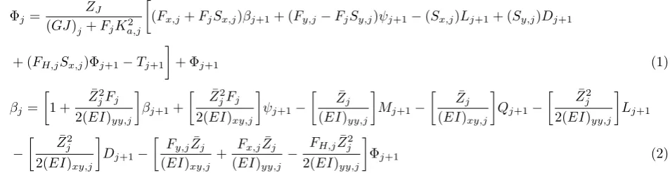
In this method, each part of the rotor blade is di-vided into smaller elements in a way that inertia is concentrated at the internal end of each part and stiff-ness is distributed along the element. Using predefine symbols for deformations, forces, and torques and us-ing free body diagram with assumption of harmonic movement and force and momentum equilibrium and continuous deformations in the entire mass, the follow-ing recursive equations were introduced [16]:

Φj =

¯

ZJ

(GJ)_j+FjKa,j2 [

(Fx,j+FjSx,j)βj+1+ (Fy,j−FjSy,j)ψj+1−(Sx,j)Lj+1+ (Sy,j)Dj+1

+ (FH,jSx,j)Φj+1−Tj+1 ]

+ Φj+1 (1)

βj = [

1 + ¯

Z2 jFj

2(EI)yy,j ]

βj+1+ [ _Z_¯2

jFj

2(EI)xy,j ]

ψj+1− [ _¯

Zj

(EI)yy,j ]

Mj+1− [ _¯

Zj

(EI)xy,j ]

Qj+1−

[ _Z_¯2 j

2(EI)yy,j ]

Lj+1

−

[ _Z_¯2 j

2(EI)xy,j ]

Dj+1− [

Fy,jZ¯j

(EI)xy,j

+ Fx,j ¯

Zj

(EI)yy,j

− FH,jZ¯j2

2(EI)yy,j ]

(4)

Ψj = [ _¯

Z_j2Fj

2(EI)xy,j ]

βi+j+ [

1 + ¯

Z_j2Fj

2(EI)xx,j ]

Ψj+1− [ _¯

Zj

(EI)xy,j ]

Mj+1− [ _¯

Zj

(EI)xx,j ]

Qj+1

−

[ _Z_¯2 j

2(EI)xy,j ]

Lj+1−

[ _Z_¯2 j

2(EI)xx,j ]

Dj+1− [

Fy,jZ¯j

(EI)xx,j

+ Fx,j ¯

Zj

(EI)xy,j −

FH,jZ¯j2

2(EI)xy,j ]

Φj+1 (3)

δy,j =− [ _F

jZ¯j3

6(EI)yy,j

+ ¯Zj ]

βj+1− [ _F

jZ¯j3

6(EI)xy,j ]

ψj+1+ (Sx,j)(ϕj−ϕj+1) +

[ _Z_¯2 j

2(EI)yy,j ]

Mj+1+

[ _Z_¯2 j

2(EI)xy,j ]

Qj+1

+

[ _Z_¯3 j

6(EI)yy,j ]

Lj+1+

[ _Z_¯3 j

6(EI)xy,j ]

Dj+1+ [ _F

y,jZ¯j2

2(EI)xy,j

+ Fx,j ¯

Z2 j

2(EI)yy,j −

FH,jZ¯j3

6(EI)yy,j ]

Φj+1+δy,j+1 (4)

δx,j =− [ _F

jZ¯j3

6(EI)xy,j ]

βj+1− [ _F

jZ¯j3

6(EI)xx,j

+ ¯Zj ]

ψj+1+ (Sy,j)(ϕj−ϕj+1) +

[ _Z_¯2 j

2(EI)xy,j ]

Mj+1+

[ _Z_¯2 j

2(EI)xx,j ]

Qj+1

+

[ _Z_¯3 j

6(EI)xy,j ]

Lj+1+

[ _Z_¯3 j

6(EI)xx,j ]

Dj+1+ [ _F

y,jZ¯j2

2(EI)xx,j

+ Fx,j ¯

Z2 j

2(EI)xy,j −

FH,jZ¯j3

6(EI)xy,j ]

Φj+1+δx,j+1 (5)

Lj=Lj+1+w2 [

(mrx)jΦj+mjδy,j ]

(6)

Dj=Dj+1+ (w2+ Ω2) [

(mry)jΦj+mjδx,j ]

(7)

Mj=Mj+1+ (Fj)(δy,j−δy,j+1)− [

Ω2Zj(mrx)j ]

Φj+ ( ¯Zj)Lj+1+ (w2+ Ω2)(Iyy,jβj+Ixy,jΨj) (8)

Qj =Qj+1+ (Fj)(δx,j−δx,i+1)− [

Ω2Zj(mry)j ]

Φj+ ( ¯Zj)Dj+1+w2(Ixy,jβj+Ixx,jψj) (9)

Tj =Tj+1+ (FH,j)(δy,j−δy,j+1) + (w2Izz,j+ Ω2TΦΦ,j)Φj+ [

(w2+ Ω2)((mry)j) ]

δX,j+ [w2(mrx)j]δy,j (10)

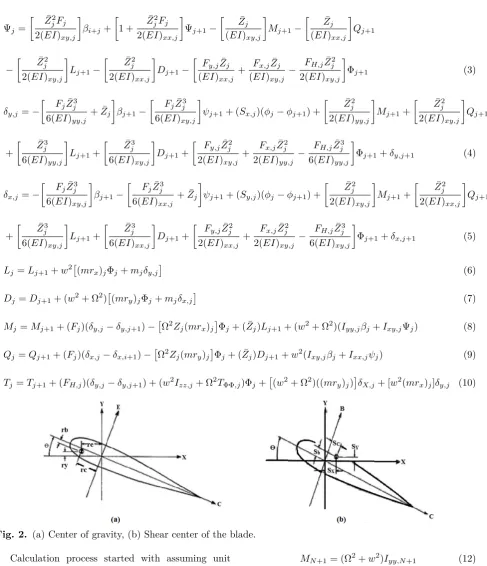
Fig. 2. (a) Center of gravity, (b) Shear center of the blade.

Calculation process started with assuming unit value for one of the deformations at the blade’s tip and zero value for other deformations. All forces and momentums at the blade’s tip can’t be equal to zero due to mass concentration. Therefore, for unit value of out-of-plane slope at the blade’s tip, forces and mo-mentums were calculated using equations (11) to (13) as below:

βN+1= 1 (11)

MN+1= (Ω2+w2)Iyy,N+1 (12)

QN+1=w2Ixy,N+1 (13) The equations in this study assume that axis of struc-ture’s main cross-section and its mass axis are parallel with each other.

(5)

axis which includes boundary conditions for collective, cyclic, and scissor modes. In all three modes, blade’s rotation around z-axis is limited using a control sys-tem.

In the Myklestad approach, half of mass and mo-ments of inertia are concentrated at the end of each part and each part is changed into an elastic structure with no mass. Deformation, moment and shear forces of internal end of each part were calculated based on deformation, moment, and shear forces of the external end of the same part. All deformations, moments, and shear forces were calculated in terms of the blade tip deformation which can ultimately result in deforma-tion, moment, and shear forces at the origin of coor-dinates. These calculations were performed using re-cursive equations. Boundary conditions were also cal-culated as a function of blade tip deformation which results in equation 14 (in which � is the vibrational fre-quency).

[C(w)]∗

     

∆ytip

Ψtip

∆xtip

βtip

Φtip     

={0} (14)

C(w)is a 5×5 matrix (4×4 if twist is eliminated).

Nat-ural frequencies are values of � which satisfy boundary conditions meaning that at these values, the determi-nant of C(w) is equal to zero. The values for Vsof t,

Vmass and Hmass are calculated using the following equations.

Vsof t=

20∗106

R∗kop

(15)

Vmass =

MHub,op

N B (16)

Hsof t=

20∗106

R∗kip

(17)

Vmass =

MHub,ip

N B (18)

Twist conditions for all modes are shown as

Φ(PHOFF)=T(PHOFF)

CK in which CK is equal to twist

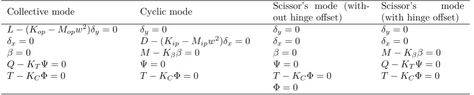
stiffness of control system. For the analysis, three main sets of boundary condition equations were used and modal results were determined in one of the collective, cyclic and scissor conditions [17]. The boundary condi-tions for each mode are shown in Table 1. Additionally, spring and mass terms are shown in Fig. 3.

(6)

Table 1

Boundary condition equations.

Collective mode Cyclic mode Scissor’s mode

(with-out hinge offset)

Scissor’s mode (with hinge offset)

L−(Kop−Mopw2)δy= 0 δy= 0 δy= 0 δy= 0

δx= 0 D−(Kip−Mipw2)δx= 0 δx= 0 δx= 0

β = 0 M −Kββ = 0 β = 0 M−Kββ = 0

Q−KTΨ = 0 Ψ = 0 Ψ = 0 Q−KTΨ = 0

T−KCΦ = 0 T−KCΦ = 0 T−KCΦ = 0 T−KCΦ = 0

Φ = 0

Collective mode is determined by vertical (out-of-plane) and horizontal (in-(out-of-plane) displacement of oppos-ing rotor blades. Suitable boundary conditions for in-plane mode are 2nd and fourth elements from first col-umn of Table 1, which are pin connection with spring coefficient of KT. First and third elements are condi-tions for clamped connection with a moving hub, which is modeled using a spring-mass system with one degree of freedom. These conditions belong to out-of-plane collective mode. First four conditions of the first col-umn in Table 1 are applied in the central line location.

Kc term shows free flexibility rate of the control sys-tem.

Cyclic mode includes in-plane symmetrical and out-of-plane asymmetrical modes around the rotational center. Boundary conditions for cyclic mode are shown in second column of Table 1. The first and third ele-ments of this column show pin conditions with flapping flexibility limit (Kβ) at the out-of-plane direction. Ele-ments 2 and 4 are for in-plane conditions, which show a stationary connection with a flexible hub (stiffness and mass characteristics of the hub are described usingMip andKip, respectively). Twist boundary conditions are similar for collective and cyclic modes.

For scissor mode, in-plane and out-of-plane bound-ary conditions at the central line show stationbound-ary con-nection of blades with an unmoving hub(δy,1=δx,1=

β1, ψ1= 0). For rotors with three or more blades, twist conditions are similar to collective and cyclic modes. For two-blade rotors, at the radial location of pitch horn connection, twist deformation is zero. These con-ditions are presented in the third column of Table 1. For in-plane and out-of-plane directions, wherever the offset of flapping and lagging hinges is desirable (such as in pin rotors), the alternative forms shown in col-umn 4 of Table 1 are used. If the offset of flap hinge is not zero, zero slope condition is replaced by an equa-tion which relates torque and slope at the hinge’s lo-cation using flapping flexibility term (Kβ). Similarly, for lag hinge offset, slope conditions for pin connection are replaced with flexibility limitKΨat the lag hinge’s location.

The calculated values of deformation, slope, mo-ment, and shear force at each part can be substituted at the left side of the boundary condition equation for each mode by satisfying relevant boundary conditions for each mode and relative to coordination with unit

being at the external edge of blade’s tip. By doing this, the equations can be used to create one column of boundary condition coefficient matrix. By repeating the substitution of relevant conditions with unite value of another dimension of the blade, the matrix is filled [18]. The terms can be derived using partial derivative of any boundary condition equations relative to specific deformation of blade tip.

Substituting calculated natural frequencies in the boundary condition matrix leads to five homogenous equations based on five unknown deformations at the end point of the blade tip. Inverse iteration approach was used to solve the blade’s tips relative deformations [19]. The inverse of coefficient matrix was multiplied with the initial guess vector. The resulting vector was used as the new guess and was again multiplied by the inverse of coefficient matrix. This was repeated four times with resulting vector being normalized us-ing the largest element. The final vector indicated the unit deformation of blade tip for that mode. Using these values and distribution of deformations, slopes, shear forces, and moments related to unit deformation of blade tip, it is possible to calculate mode shapes, shear force and moment distributions. Shear forces and moments were solved again at the local coordi-nation system of each part using twist and collective pitch angle.

To calculate mode shapes, it was assumed that

∆y= 1; subsequently 4 boundary condition equations were soleved (eliminating twist leads to 3 equations) in order to determine deformation at the blade’s tip. Since all deformations, moments, and forces were func-tions of deformation, it was possible to calculate mode shapes. Then, mode shapes were normalized relative to largest linear deformation value or a 10-degree twist. Finally, all mode shapes were drawn at different direc-tions.

3. Implementation in MATLAB

Soft-ware

Using the abovementioned method, an application pro-gram was coded in MATLAB environment for extract-ing natural frequencies of rotor blade and drawextract-ing mode shapes.

(7)

of 1 and was included in calculations (this value can-not be changed by the user). The user can enter the necessary parameters about static and dynamic char-acteristics of rotor. In the next stage, the number of nodes in hub was calculated. Then, the angular veloc-ity of the rotor which was entered in rounds per minute was converted to Radian per second and its square was calculated. In the next stage, rotor collective pitch an-gle was calculated and used for later calculations. N is the number of elements andN1 shows the number of nodes. Next, pitch angle of each node was calculated by multiplying the size of each element by torsion rate and was then converted from degrees to Radian. Then Rotor collective pitch angle was converted to Radian and angular velocity was also converted to radian per second. In the next step, mass inertia of flap and mass of the end of the blade was calculated. After calcu-lating half of element mass before and after the node, product of mass with center of mass distance and shear center and inertia of mass moment were calculated in the longitudinal and transverse directions. In order to create the coefficient matrix, each time, one of theβ,

x, y, Ψand Φvalues was set to 1 with the rest equal to zero (which is one of the theoretical necessities for Myklestad approach). In the next step, the average angle of two elements was calculated, and was added to the root collective angle and then was calculated at the end of the blade in the direction perpendicular to x and y axis for unit force.

Centrifugal forces and moments related to distance from center of gravity were calculated in the reference coordination system. It is worth mentioning that these forces and moments were calculated from blade’s tip toward its base.

The next step was calculating non-zero terms at the blade’s tip. Then, boundary conditions were used to create the boundary condition matrix. At the first line, one of the elements of coefficient matrix was defined as a symbolic value, so MATLAB can define the matrix as a symbolic matrix. After that, coefficient matrix for collective boundary conditions was calculated based on frequency variable. At the end of the program, the natural frequencies of the rotor blade were stored in another matrix in terms of Hz and sorted in ascending order. After calculating the natural frequencies, it is necessary to draw mode shapes of the rotor blade at these calculated frequencies. As a result, the program was used to draw torsion, vertical, and horizontal mode shapes for collective, cyclic, and scissor boundary con-ditions.

4. Validation of Results Using Finite

El-ement Method

After preparation of vibration code in MATLAB envi-ronment, it is required to validate the output results

of the program. To this end, numerical simulation and vibrational analysis of a beam with different material and geometrical conditions by clamp support was car-ried out as three problems in Patran software. The results include natural frequencies and mode shapes of the structure. Based on the boundary conditions for scissor condition, the boundary condition was consid-ered to be similar to those for clamped support condi-tions (Fig. 1).

4.1. Problem Definition

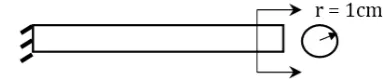
In the first problem, an aluminum beam with length of 1 meter and circular cross-section was considered as seen in Fig. 4. This beam was divided into 20 parts for vibrational analysis problem.

Fig. 4. Schematic of the first problem.

By assuming ρ = 2700 kg⁄m3 _{for aluminum and} the problem’s geometry, the mass of beam and each element was calculated as 0.8478 and 0.04239 kg, re-spectively. Due to the asymmetrical cross-section of the beam, we have:

rb=rb=Sb=Sc= 0

Second moment of area and polar moment of inertia were also calculated as 0.785 ×10−8m4 _and ₁_.₅₇_×

10−8m4 _{respectively.}

By considering ν = 0.33, E = 70GPa and G =

E

2(1 +ν) = 26.31GPa for aluminum, bending and

tor-sion stiffness of the beam were calculated using the following equation:

EI = 70×109×0.785×10−8= 549.5N.m2

GJ = 26.31×109×1.57×10−8= 413.07N.m2 Second mass moment of inertia for each part was cal-culated along beam-wise and chord-wise length of the blade using the following equation:

Ibb=Icc=

1 12ml

2₌ 1

120.04239×0.05

2

= 0.883125×10−5kg.m2

(8)

Fig. 5. Schematic of the second problem.

In order to validate the accuracy of the code for a rotating beam with variable mass and geometrical properties along its length, the next problem investi-gated a rotating beam with variable mass and geomet-rical properties.

In the third problem, an aluminum beam with length of 61cm with variable cross-section was consid-ered, rotating with the angular velocity of 1000 rpm. In order to analyze the vibrations, the beam is divided

into 22 parts. The schematic of this beam was shown in Fig. 6.

Fig. 6. Schematic of the third problem’s beam.

4.2. Solution with MATLAB Software

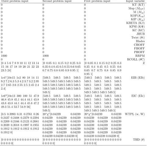
After calculating geometrical and mass characteristics, vibrational analysis of these beams was carried out us-ing the code created in the previous section. The inputs of vibration code of the problem are shown in Table 2.

Table 2

Program input of first problem beam to third problem beam.

Third problem input Second problem input First problem input Input variable

0 0 0 KT (KT)

0 0 0 Mop (MOP)

0 0 0 M (Mip)

0 0 0 KOP(Kop)

0 0 0 KIP (Kip)

0 0 0 KBETA (Kβ)

0 0 0 KPSI (KΨ)

0 0 0 KC (KC)

0 0 0 JHUB

0 0 0 Twist (θt)

0 0 0 Blades

0 0 0 CHOFF

0 0 0 FHOFF

0 0 0 PHOFF

1000 1000 0 RRPM

0 0 0 RCOLL (θC)

[0 4 5 6 7 8 9 10 11 12 13 14 15 16 17 18 19 20 21 22 23 23.5 24]

[0 0.05 0.1 0.15 0.2 0.25 0.3 0.35 0.4 0.45 0.5 0.55 0.6 0.65 0.7 0.75 0.8 0.85 0.9 0.95 1]

Z

1e4∗[10e15 1e2 80 18 14 11 9.2 7.2 6.3 5.3 4.2 3.7 3.2 2.95 2.7 2.65 2.6 2.55 2.5 2.45 2.4 2.4]

[549.5 549.5 549.5 549.5 549.5 549.5 549.5 549.5 549.5 549.5 549.5 549.5 549.5 549.5 549.5 549.5 549.5 549.5 549.5 549.5]

EIB (EIb)

1e6*[10e13 300 100 51 47.9 46.8 45.8 45.1 44.4 44.1 43.8 43.8 43.8 44.1 44.4 45.8 47.2 49.3 51.4 53.7 54.9 56]

[549.5 549.5 549.5 549.5 549.5 549.5 549.5 549.5 549.5 549.5 549.5 549.5 549.5 549.5 549.5 549.5 549.5 549.5 549.5 549.5]

EIC (EIc)

[0.5 0.3993 0.31 0.2761 0.26 0.2437 0.2408 0.2379 0.2294 0.2209 0.2166 0.2123 0.2081 0.2039 0.2018 0.1997 0.1955 0.1912 0.1912 0.1912 0.1912 0.1912 0]

20∗g∗[0.04239 0.04239 0.04239 0.04239 0.04239 0.04239 0.04239 0.04239 0.04239 0.04239 0.04239 0.04239 0.04239 0.04239 0.04239 0.04239 0.04239 0.04239 0.04239 0.04239 0]

WTPL (w, W)

[0 0 0 0 0 0 0 0 0 0 0 0 0 0 0 0 0 0 0 0]

(9)

Third problem input Second problem input First problem input Input variable 1e-2∗[0.25∗266.7 3.327 2.583

2.301 2.167 2.031 2.007 1.983 1.912 1.841 1.805 1.769 1.734 1.699 1.682 1.664 1.629 1.593 1.593 1.593 2*0.1992 2*0.1991]/g

0.883125e-5∗20∗[1 1 1 1 1 1 1 1 1 1 1 1 1 1 1 1 1 1 1 1]

EYBC (ICC)

1e6∗[10e12 1 0.7 0.575 0.48 0.42 0.382 0.348 0.32 0.295 0.275 0.261 0.251 0.241 0.23 0.214 0.196 0.173 0.153 0.125 0.1 0.078]

413.07∗[1 1 1 1 1 1 1 1 1 1 1 1 1 1 1 1 1 1 1 1]

GJ

[0 0 0 0 0 0 0 0 0 0 0 0 0 0 0 0 0 0 0 0]

SB (Sb)

[0 0 0 0 0 0 0 0 0 0 0 0 0 0 0 0 0 0 0 0]

SC (SC)

[0 0 0 0 0 0 0 0 0 0 0 0 0 0 0 0 0 0 0 0]

RB (rb)

[0 0 0 0 0 0 0 0 0 0 0 0 0 0 0 0 0 0 0 0]

RC (rC)

4.3. Solution Using Patran Software

Based on the determined characteristics, these beams were also modeled and analyzed in Patran software. The results of numerical simulation and vibration code in Lag and Lead directions for these three problems are shown in Tables 3, 4 and 5, respectively.

After calculating the natural frequencies of the beams, it is necessary to draw the mode shape of the frequencies at Lag and Lead directions for numerical simulation and vibration code; subsequently, compar-ing the results is essential.

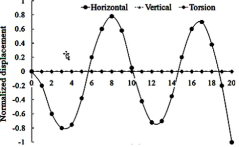
Based on the results, for the first problem, Fifth mode shape of the beam at lag and lead direction for numerical simulation and vibration code is shown in Figs. 7 and 8, respectively. For the second problem, Fourth mode shape of the beam at the lag direction for numerical simulation and vibration code is shown in Figs. 9 and 10, respectively. For the third problem, Fourth mode shape of the beam at the lag direction for numerical simulation and vibration code is shown in Figs. 11 and 12, respectively.

Fig. 7. Fifth horizontal mode shape of first problem beam resulting from numerical simulation.

5. Results

After calculating geometrical and mass characteristics of the beam, vibrational analysis was carried out us-ing the code introduced in the previous section. Then the results were compared to the results of numerical simulation.

For the first problem, as seen in Table 3, the re-sults of vibration code have a good compatibility with the results of numerical simulation. This compatibility shows that the code is useable for a beam with constant cross-section and without angular velocity.

Based on Figs. 7 and 8, the lag and lead mode shapes are exactly alike with mode shapes acquired from numerical simulation and vibration code for both directions, which are also compatible with each other.

Fig. 8. Fifth horizontal mode shape of first beam re-sulting from modal analysis.

Fig. 9. Fourth vertical mode shape of second problem beam resulting from numerical simulation.

(10)

good compatibility with numerical simulation. How-ever, there is significant error at mode number 1 in the lag condition. Since other errors are close to 4%, this data point can be considered an outline result. The rest of the compatible results indicate that the code is ap-plicable for rotating beam with constant cross-section. According to Figs. 9 and 10, Lag mode shapes are exactly similar to mode shapes calculated from numer-ical simulation and vibration code, which are compat-ible with each other.

Fig. 10. Fourth vertical mode shape of second prob-lem beam resulting from modal analysis.

Fig. 11. Third vertical mode shape of third beam problem resulting from numerical simulation

Fig. 12. Third vertical mode shape of third beam problem resulting from modal analysis.

Table 3

Natural frequency resulting from numerical simulation and modal analysis for first beam.

Error percentage Patranwn(Hz) MATLABwn(Hz) _Mode

Horizontal Vertical Horizontal Vertical Horizontal Vertical

0 0 14.228 14.228 14.223 14.223 1

0.4 0.4 88.824 88.824 88.381 88.381 2

1.2 1.2 247.67 247.67 244.631 244.631 3

2.24 2.24 482.88 482.88 472.063 472.063 4

3.47 1.8 793.55 780.32 765.97 765.97 5

Table 4

Natural frequency resulting from numerical simulation and modal analysis for second problem beam.

0.4 31.26 23.089 23.089 22.998 15.87 1

2.62 1.2 99.163 99.163 96.563 97.954 2

2.23 2.03 259.68 259.68 253.881 254.394 3

3.04 3.09 497.45 497.45 482.03 482.04 4

4.26 4.28 811.2 811.2 776.57 776.42 5

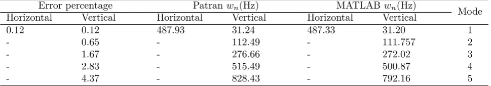
Table 5

Natural frequency resulting from numerical simulation and modal analysis for third problem beam.

0.12 0.12 487.93 31.24 487.33 31.20 1

- 0.65 - 112.49 - 111.757 2

- 1.67 - 276.66 - 272.02 3

- 2.83 - 515.49 - 500.87 4

(11)

For the third problem, based on the results pre-sented in Table 5, the results acquired from vibration code have good compatibility with the results of nu-merical simulation. This compatibility shows that the code is applicable for a rotating beam with variable cross-section.

6. Conclusions

This application can be used to estimate natural fre-quencies and mode shapes of helicopter rotor blades. This application is based on Holzer – Myklestad ap-proach on a rotating beam which represents rotor blades with a series of concentrated masses connected together using stiffness elements. Elasticity and cou-pled inertia between horizontal, vertical, and twist cur-vature were considered in the analysis. The set of structural stiffness, mass, blade torsion, torsion iner-tia and distance from center of mass and distance be-tween shear center and twist axis can be used as limits of this problem. These limits are usually used to show different hubs on mode shapes. The precision of results was shown by comparing the results to numerical ones. The calculated bending frequency has good compati-bly with the measured results with 4.26% error. The presented program can be used to achieve the blade’s natural frequencies in coupled loading condition. The other codes can only calculate the natural frequencies for one case on loading like bending moment. So this unique program can be used to measure the coupled natural frequencies for different kinds of rotor blades with different boundary conditions.

References

[1] C. Houbolt, G.W. Brooks, Differential equations of motions for combined flap wise bending and torsion of twisted non-uniform rotor blades, NACA Report 1346, (1958).

[2] R.L. Bielawa, Rotary wing structural dynamics and aeroelasticity, American Institute of Aeronautics and Astronautics (AIAA) Education Series, Wash-ington, D.C. AIAA Inc, (1992).

[3] A.D. Wright, C.E. Smith, R.W. Thresher, J.L.C. Wang, Vibration modes of centrifugally stiffened beams, ASME J. Appl. Mech., 49(1) (1982) 197-202.

[4] G. Surace, V. Anghel, C. Mares, Coupled bending-bending-torsion vibration analysis of rotating pretwisted blades: an integral formulation and nu-merical examples, J. Sound. Vib., 206(4)4 (1997) 473-486.

[5] S.M. Lin, The instability and vibration of rotating beams with arbitrary pretwist and an elastically

re-strained root, ASME J. Appl. Mech., 68(6) (2001) 844-853.

[6] S.M. Lin, S.Y. Lee, W.R. Wang, Dynamic anal-ysis of rotating damped beams with an elastically restrained root, Int. J. Mech. Sci., 46(5) (2004) 673-693.

[7] S.Y. Lee, S.M. Lin, T. Wu, Free vibrations of rotat-ing non-uniform beam with arbitrary pretwist, An elastically restrained root and a tip mass, J. Sound. Vib., 273(3) (2004) 477-492.

[8] S. Newman, The Foundations of Helicopter Flight, Butterworth-Heinemann, Elsevier, (1994).

[9] Headquarters, U.S. Army Materiel Command, En-gineering design handbook for helicopter engineer-ing (AMCP 706-201) Part I, Preliminary Design, (1974).

[10] A.R.S. Bramwell, D. Balmford, G. Done, Heli-copter Dynamics, Butterworth-Heinemann, Else-vier, (2001).

[11] S. Graham Kelly, I. Morse, R.T. Hinkle, Mechan-ical Vibrations Theory and Applications, Cengage, (2012).

[12] P. Skalski, Testing of a composite blade, Acta Mech. Autom., 5(4) (2011) 101-104.

[13] S. Rizo-Patron, J. Sirohi, Operational modal anal-ysis of a helicopter rotor blade using digital image correlation, Exp. Mech., 57(3) (2017) 367-375.

[14] A. Teter, J. Gawryluk, Experimental modal analy-sis of a rotor with active composite blades, Compos. Struct., 153 (2016) 451-467.

[15] P. Sarker, R.C. Theodore, K. Chakravarty, Vibra-tion analysis of a composite helicopter rotor blade at hovering condition, Adv. Aero. Tech., 1 (2016) 1-10.

[16] R.L. Bennett, Digital computer program DF1758 fully coupled natural frequencies and mode shapes of a helicopter rotor blade, NASA-CR-132662, (1975).

[17] R.L. Bennett, Rotor system design and evalua-tion using a general purpose helicopter flight sim-ulation program, Specialists meeting on helicopter rotor loads prediction methods, Defense Technical Information Center, (1973).

[18] S.G. Sadler, Informal Final report on blade fre-quency program for nonuniform Helicopter rotors, with Automated Frequency Search, NASA CR-112071, (1972).