https://doi.org/10.5194/gmd-12-4133-2019 © Author(s) 2019. This work is distributed under the Creative Commons Attribution 4.0 License.
Identification of key parameters controlling demographically
structured vegetation dynamics in a land surface model:
CLM4.5(FATES)
Elias C. Massoud1,2, Chonggang Xu3, Rosie A. Fisher4, Ryan G. Knox5, Anthony P. Walker6, Shawn P. Serbin7, Bradley O. Christoffersen8, Jennifer A. Holm5, Lara M. Kueppers5, Daniel M. Ricciuto6, Liang Wei3,
Daniel J. Johnson9, Jeffrey Q. Chambers5, Charlie D. Koven5, Nate G. McDowell10, and Jasper A. Vrugt2,11
1Jet Propulsion Laboratory, California Institute of Technology, Pasadena, CA, USA
2Department of Civil and Environmental Engineering, University of California Irvine, Irvine, CA, USA 3Earth and Environmental Sciences Division, Los Alamos National Laboratory, Los Alamos, NM, USA 4Centre Européen de Recherche et de Formation Avancée en Calcul Scientifique (CERFACS), Toulouse, France 5Climate and Ecosystem Sciences Division, Lawrence Berkeley National Laboratory, Berkeley, CA, USA 6Environmental Sciences Division, Oak Ridge National Laboratory, Oak Ridge, TN, USA
7Environmental & Climate Sciences Department, Brookhaven National Laboratory, Upton, NY, USA 8Department of Biology, University of Texas Rio Grande Valley, Edinburg, TX, USA
9School of Forest Resources and Conservation, University of Florida, Gainesville, FL, USA
10Earth Systems Analysis and Modeling Division, Pacific Northwest National Laboratory, Richland, WA, USA 11Department of Earth System Science, University of California Irvine, Irvine, CA, USA
Correspondence:Chonggang Xu ([email protected])
Received: 8 January 2019 – Discussion started: 7 February 2019
Revised: 9 August 2019 – Accepted: 16 August 2019 – Published: 23 September 2019
Abstract. Vegetation plays an important role in regulating global carbon cycles and is a key component of the Earth system models (ESMs) that aim to project Earth’s future cli-mate. In the last decade, the vegetation component within ESMs has witnessed great progress from simple “big-leaf” approaches to demographically structured approaches, which have a better representation of plant size, canopy structure, and disturbances. These demographically structured vege-tation models typically have a large number of input pa-rameters, and sensitivity analysis is needed to quantify the impact of each parameter on the model outputs for a bet-ter understanding of model behavior. In this study, we con-ducted a comprehensive sensitivity analysis to diagnose the Community Land Model coupled to the Functionally Assem-bled Terrestrial Simulator, or CLM4.5(FATES). Specifically, we quantified the first- and second-order sensitivities of the model parameters to outputs that represent simulated growth and mortality as well as carbon fluxes and stocks for a trop-ical site with an extent of 1×1◦. While the photosynthetic capacity parameter (Vc,max25) is found to be important for
simulated carbon stocks and fluxes, we also show the impor-tance of carbon storage and allometry parameters, which de-termine survival and growth strategies within the model. The parameter sensitivity changes with different sizes of trees and climate conditions. The results of this study highlight the im-portance of understanding the dynamics of the next gener-ation of demographically enabled vegetgener-ation models within ESMs to improve model parameterization and structure for better model fidelity.
1 Introduction
com-ponent of ESMs, are capable of representing vegetation dy-namics through the use of dynamic global vegetation models (Foley et al., 1996; Cox et al., 2000; Krinner et al., 2005; Friedlingstein et al., 2006; Sato et al., 2007; Arora et al., 2013). The first-generation dynamic vegetation models rep-resent plant communities and their competition using a sin-gle area-averaged representation of plant functional types (PFTs) within each land grid cell (Cox et al., 2000; Pan et al., 2002; Hickler et al., 2004). Recently, a number of vegeta-tion models that can represent plant demographic processes have emerged to better capture coexistence and competition driven by light competition between different sizes of trees within a vertical canopy structure at different successional stages (Moorcroft et al., 2001; Thonicke et al., 2001; Sitch et al., 2003; Hickler et al., 2004; Fisher et al., 2010; Scheiter et al., 2013; Fisher et al., 2018). These demographic mod-els allow comparison with many more observed vegetation processes than first-generation models but also contain more degrees of freedom leading to great complexity.
LSMs typically contain a suite of different parameters to resolve the carbon, water, and energy fluxes and pools at the land–atmosphere interface (Noilhan and Planton, 1989; Bastidas et al., 1999; Gupta et al., 1999; Masson et al., 2003; Sargsyan et al., 2014). Many of these parameters can be es-timated directly in the field, but others are difficult or im-possible to measure due to various complications such as the abstract representation of processes, technological limita-tions, or spatial/temporal aggregation (Entekhabi and Eagle-son, 1989; Kumar et al., 2006). Parameters that are observ-able in the field are also often subject to large natural variabil-ity, including changes through space and time (Wood et al., 1992; Masson et al., 2003; Fisher et al., 2015). For exam-ple, vegetation parameters can be used to describe different root profiles (Vrugt et al., 2001; Zeng, 2001; Massoud et al., 2019a) or photosynthetic capacities (Leuning, 2002; Rogers, 2014); however, model parameter values are often taken from literature publications or databases, and may not represent local variation or capture seasonal or ontogenetic changes. For parameters of critical importance, even a small difference can lead to significant divergence for multi-model ensemble projections or uncertainty in model predictions from differ-ent models (Sitch et al., 2008; Dietze et al., 2014; McDowell et al., 2016; Rogers et al., 2017). Since parameters are often defined in simulations with limited prior knowledge of their mean values and variation (O’Hagan and Leonard, 1976; Ki-tanidis, 1986; Geromel, 1999), model uncertainty or sensitiv-ity analyses are typically required to adequately quantify the uncertainty in model outputs and importance of parameters to guide model calibration and improvement.
There are two types of uncertainty and sensitivity analysis studies. One type of study aims to understand the model be-haviors by exploring the baseline sensitivity of model outputs to parameter changes, which is normally an equal amount of deviation from the mean values of default parameters. This is commonly referred to as model sensitivity or elasticity
anal-ysis (e.g., Benton and Grant, 1999; Pappas et al., 2013; Men-berg et al., 2016; Collalti et al., 2019). Another type of study aims to quantify the amount of uncertainty in model out-puts and the corresponding contributions to this uncertainty by different sources, which is commonly referred to as un-certainty quantification (e.g., Xu et al., 2010; Dietze et al., 2014). It is possible that a model output is very sensitive to a particular parameter in the sensitivity analysis study, but the parameter could contribute to a small amount of uncer-tainty in the model output if this parameter contains a low level of variation (Dietze et al., 2014). Both types of studies are useful for model development and applications with sen-sitivity analysis studies focusing on understanding the base-line of model behaviors and uncertainty quantification stud-ies focusing on guiding field and laboratory measurements. Despite the need for such studies, systematic investigation of the parameter sensitivity and output uncertainty of LSMs is not standard practice, potentially on account of the high dimensionality involved (although see Zaehle et al., 2005; Fisher et al., 2010; Pappas et al., 2013).
The goal of this study is to conduct a comprehen-sive sensitivity analysis for a land surface model (Com-munity Land Model) coupled to a demographic vegetation model (Functionally Assembled Terrestrial Simulator), or CLM4.5(FATES), at a tropical site with an extent of 1×1◦ to (1) understand the baseline model behaviors of vegetation carbon stocks and fluxes and vegetation demography in rela-tion to different model parameters, and (2) provide direcrela-tions for improved model parameterization toward a better model fit to observations. Specifically, we aim to answer the follow-ing question: what are the main parameter controls on vege-tation processes such as growth and mortality and on the re-sulting dynamics of carbon fluxes and stocks? Based on our understanding of simulated processes in CLM4.5(FATES), we propose to test three hypotheses. Our first hypothesis is related to photosynthetic capacity. The carbon input for veg-etation growth is through photosynthesis and in most LSMs, it is simulated based on the Farquhar model (Farquhar, 1989) with the photosynthetic capacity represented by the maxi-mum carboxylation rate at 25◦C (Vc,max25) and maximum
electron transport rate at 25◦C (Jmax25).Jmax25is simulated
in proportion toVc,max25in many models, and previous
sen-sitivity analysis studies (Pappas et al., 2013; Sargsyan et al., 2014; Dietze et al., 2014) have shown that Vc,max25is
gen-erally an important parameter that affects simulated carbon fluxes. Therefore, we hypothesize that the photosynthetic ca-pacity parameter, Vc,max25, is a key control on simulated
carbon fluxes in CLM4.5(FATES) (H1). Second, for demo-graphic models, the allometry of trees determines the amount of carbon input to different tissues (e.g., leaf, root, and stem). If more carbon is allocated to leaf compared to stem, the tree will have a higher productivity but this can also lead to lower stem growth and thus less height growth for light compe-tition. Thus, we hypothesize that allometry parameters are important for vegetation growth and long-term carton stocks (H2), as they will determine plant’s growth strategies. Fi-nally, the carbon stock for vegetation is affected not only by the input of carbon through photosynthesis but also by the loss of carbon through mortality. We hypothesize that the pa-rameters determining mortality are important drivers of the long-term vegetation carbon stocks (H3), as they will control carbon turnover time.
2 Materials and methods 2.1 CLM4.5(FATES)
CLM4.5(FATES) is an open-source land surface model cou-pled with a demographically structured dynamic vegetation model designed to predict climate–vegetation interactions. The land surface Community Land Model (CLM) represents surface heterogeneity and simulates land biogeophysics, the hydrologic cycle, biogeochemistry, human dimensions, and ecosystem dynamics (Oleson et al., 2013). It is used within
various Earth system modeling frameworks, including the Community Earth System Model (CESM) and the Norwe-gian Earth System Model (NorESM) (Lawrence et al., 2011; Bonan et al., 2011). It is also the baseline of the land com-ponent within the Exascale Energy Earth System Model (E3SM) (Golaz et al., 2019). The vegetation model FATES is developed from the ecosystem demography (ED) model, which scales up the behavior of forest ecosystems by ag-gregating individual trees into representative “cohorts” based on their size and PFT, and by aggregating groups of cohorts into representative “patches” (conceptually similar to a for-est plot) that explicitly tracks the time between disturbances (Moorcroft et al., 2001). The main property of the ED con-cept that differs from most commonly used “big-leaf” mod-els is the capacity to predict distribution, structure, and com-position of vegetation directly from their given physiolog-ical traits described by the model parameterization (Fisher et al., 2015). This is achieved via the means of trait filtering, whereby plant traits affect plant growth and survival, growth in turn affects the acquisition of light resources, and feeds back onto growth, survival, and reproduction. Differences in growth, survival, and reproduction rates thus directly con-trol the relative distributions of vegetation types and their traits as well as the overall carbon stocks. See supplementary model description in Fisher et al. (2015) for details on spe-cific components of the model structure. FATES represents vegetation using size-structured groups of plants (cohorts) which coexist on various successional trajectory-based land units. FATES simulates growth by integrating photosynthesis across different leaf layers for each cohort. The model allo-cates photosynthetic carbon to different tissues such as leaf, root, and stem based on the allometry of different vegetation types. Mortality is an important driver for the simulated for-est dynamics in FATES. FATES includes five modes of mor-tality: (1) fixed background mortality, (2) hydraulic failure based on a threshold of very low soil moisture; (3) carbon starvation resulting from the depletion of carbon storage in plants (see Appendix C for details); (4) impact mortality re-sulting from the falling of big trees; and (5) fire (Fisher et al., 2015). CLM and FATES are coupled to exchange carbon and water between vegetation and soil through a common inter-face. FATES is designed to be modular and currently can be turned on within two land surface models: the CLM and E3SM land model (ELM). Depending on the purpose of dif-ferent studies, CLM4.5(FATES) can be simulated with differ-ent modes including point mode for individual sites, regional mode for watershed or regional scales, and global mode for the global scale.
tree PFT, which is a typical vegetation type for the study re-gion (the Amazon). We want to point out that, because of the high species diversity in the tropics, it is always a challenge for models to capture diverse traits with a limited number of PFTs in typical ESMs. By limiting our sensitivity anal-ysis to one PFT in this study, our sensitivity analanal-ysis will help us understand the main control on demographic rates of growth and mortality that will essentially affect the outcome of competition for multiple PFTs. Thus, we expect that our sensitivity analysis can be used to guide the selection of traits for the representation of trait trade-off for diverse tropical forests and to improve the simulation of PFT coexistence for model calibration and improvement. Second, the model gen-erally underestimates leaf area index (LAI). We expect that our sensitivity analysis will be used as a guidance to adjust identified key model parameters in order to better fit model predictions to the observations.
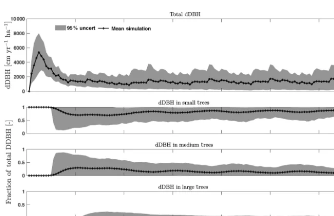
The CLM4.5(FATES) tracks different size classes of plants (generally >10 size classes) through time. To fa-cilitate our analysis, we aggregate cohorts into three size categories: small (<10 cm), medium (10–50 cm), and large trees (>50 cm). For sensitivity analysis of each size cate-gory (small, medium, and large trees), we choose to aver-age the outputs over 30-year intervals. This is done with the view that a large amount of variability in model outputs could be caused by the transient and abrupt changes across size classes, and thus only a small amount of variability is af-fected by parametric variations. Our analysis shows that the identified key parameters and the corresponding magnitude of sensitivity are similar with averaging over different num-bers of years from 20 to 40 years (Fig. D1).
2.2 Sensitivity analysis: the FAST method
Global sensitivity analysis aims at quantifying the contri-butions of input variables to the variability of the outputs of a physical model by simultaneously sampling values of parameters from their corresponding statistical distributions. There are many methods for global sensitivity analysis. Two popular variance-based approaches are the Sobol method (Sobol’, 1990) and the Fourier amplitude sensitivity test (FAST) (Cukier et al., 1973). The Sobol method has received much attention since it provides a clear description of the importance index of model parameters based on variance de-composition. However, the full description requires the eval-uation of 2nMonte Carlo integrals (Sudret, 2008), which is not practically feasible unlessnis low (nhere represents the dimensionality of the model or the number of active param-eters). Compared to Sobol’s method, FAST is more compu-tationally efficient. It can be used effectively for nonlinear and nonmonotonic models (Sudret, 2008; Xu and Gertner, 2011a). FAST uses a periodic sampling approach to draw samples from the parameter space defined by probability dis-tributions with a characteristic periodic signal for each pa-rameter. These samples will then be fed into the model for
ensemble simulations. Finally, a Fourier transformation is applied to decompose the variance of a model output into partial variances contributed by different model parameters based on the characteristic periodic signal assigned for each parameter. Only the first-order sensitivity indices referring to the “main effect” of parameters were calculated in the original method. In the 1990s, an extended FAST method able to calculate sensitivity indices referring to “total effect” was developed (Sobol’, 1990; Archer et al., 1997; Saltelli et al., 1999). This “total effect” of a parameter’s sensitiv-ity refers to the sum of a parameter’s individual contribution (first-order sensitivity) and the contribution from its interac-tion with other parameters (higher-order sensitivity) on the overall variance of the model output; that is, the total effect includes all the higher-order interactions. Xu and Gertner (2011a) further derived equations within the FAST frame-work to calculate specific higher-order interactions for dif-ferent sampling approaches. The FAST method has found widespread use in many different fields of study including sensitivity analysis of the parameters of models that repre-sent the land surface (Collins and Avissar, 1994), chemical reaction (Haaker and Verheijen, 2004), nuclear waste dis-posal (Lu and Mohanty, 2001), erosion (Wang et al., 2001), hydrologic systems (Francos et al., 2003), atmospheric sys-tems (Kioutsioukis et al., 2004), crop growth (Wang et al., 2013), or matrix population and forest landscape models (Xu and Gertner, 2009; Xu et al., 2009).
In this study, we quantify both the first- and second-order sensitivities of the model parameters using FAST. It is possi-ble to identify higher-order interactions with FAST; however, because of the sample size limitations for a larger trivariate parameter space, the FAST-based estimation of third-order sensitivity indices would be less reliable (Xu and Gertner, 2011a). Specifically, the first-order sensitivity is used to mea-sure the importance of the variations in one parameter to the model outputs. If one parameterxi is important to a model
outputy at timet (i.e.,y(t )), we expect that the mean value
ofy(t )will change substantially with different values ofxi.
Statistically, we expect to see a large variance of the expected value ofy(t )givenxi(i.e., largeV
E y(t )|xi
, whereE · is the expected value of the output,V·is the variance cal-culated in the parameter space). Similarly, if the combined impact ofxi andxj is important, we expect to see a large
variance of the expected value ofy(t )givenxi andxj (i.e.,
largeVE y(t )|xi, xj
). Therefore, we calculate the first-and second-order sensitivities,αxiandαxixj, respectively, of
time step as follows:
αxi(t )=
VE y(t )|xi
V (y(t )) (1)
αxi,xj(t )=
V
E y(t )|xi, xj
−V
E y(t )|xi
−V
E y(t )|xj
V
y(t )
,
i6=j, (2)
where Vy(t )is the total variance of model output y(t ). In FAST, the variances are estimated through periodic sam-ples in the θ space between 0 and 2π, which are linked to the samples in the parameter space through a search func-tion. Further details on the FAST toolbox used for this study can be found in Xu and Gertner (2007, 2009, 2011a) or Xu et al. (2009). We are aware that FAST can provide ro-bust estimates of the sensitivity coefficients in high dimen-sions (Wang et al., 2013), especially since the CPU demands of CLM4.5(FATES) mandates application of a method like FAST due to its ability to derive sensitivity values with sparse sampling. Due to the random parametric sampling, there will be errors in the estimates of sensitivity indices. In this study, we estimate the standard error of FAST-based sensitivity in-dex derived by Xu and Gertner (2011b), with lower errors for a larger sample size.
To better understand how parameters affect specific CLM4.5(FATES) output variables (i.e., the relationship be-tween model parameters and outputs), we also fitted cubic splines to the scatterplots between samples of parameters identified as important by FAST and the corresponding out-put variable of interest using the R SemiPar package (Rup-pert et al., 2003).
2.3 Parameter selection
In total, there are more than 200 parameters for all land sur-face processes including sursur-face energy exchange, hydrol-ogy, biogeochemistry, plant physiolhydrol-ogy, and demographic processes within CLM4.5(FATES). In this study, we focus solely on vegetation components and select 87 parameters that are relevant to vegetation processes, including parame-ters for photosynthetic processes, temperature response, al-lometry description, radiative transfer, recruitment, turnover, and mortality. See Tables D1–D4 in the Appendix for a com-plete list of the parameters used in this study, with cor-responding description, units, default values, and applied ranges. Refer to Appendix A for the allometry equations, Ap-pendix B for the temperature response curve (photosynthe-sis) equations, and Appendix C for the carbon storage equa-tions used in CLM4.5(FATES).
To conduct the sensitivity analysis, we have extracted many parameters in the model that were “hard-wired” in CLM4.5(FATES). The FAST algorithm requires valid ranges
Figure 1.Recycled climate drivers for the study area including an-nual mean precipitation, relative humidity, and air temperature for the years 1948–1972. The annual radiation and air pressure are not plotted as they are quite stable across years.
to be chosen for each parameter, which creates the possible parameter space to sample from. In theory, each parameter has a corresponding observational distribution that produces the ideal space for sampling (LeBauer et al., 2013). How-ever, in this study, there are both a large parameter set and a scarcity of appropriate data sources for Amazonian forests for many of the relevant quantities; therefore, obtaining a ro-bust data-supported distribution for each parameter was dif-ficult. Because we only aim to understand the baseline model structure, the parameter ranges in this study were generated by applying a uniform distribution over a range that spans ±15 % of the default parameter values of CLM4.5(FATES) (i.e., default parameter values for tropical evergreen trees). We choose a rather conservative range of±15 % of the de-fault CLM4.5(FATES) values so that global sensitivity in-dices can be estimated in the reasonable vicinity of the de-fault parameters. We suggest that a more robust uncertainty analysis based on realistic parameter ranges is needed for guidance on additional field measurements.
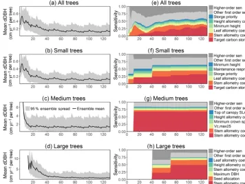
Figure 2.Simulated temporal dynamics in diameter at breast height (dDBH; cm yr−1tree−1) and the corresponding first-order parametric sensitivity indices. The left panels show the simulated ranges of dDBH for(a)all,(b)small (diameter <10 cm),(c)medium (10 cm < diameter<50 cm), and(d)large trees (diameter>50 cm). Shown is the mean simulation (black line) with 95 % spread of the simulation ensemble. Right panels show the sensitivity for the top six most important parameters for (e)density of all trees,(f)small tree density,
(g)medium tree density, and(h)large tree density, in order of importance based on the mean parametric sensitivity across years (red is the most important and blue is the least important). The jumps seen in 10, 40, 70, and 100 years for small, medium, and large trees are due to the temporal averaging mentioned in the materials and methods section. The figures also show sensitivities of the remaining parameters in light grey (first-order sensitivity index for all other parameters) as well as the sensitivity of parameter interactions in dark grey (higher-order sensitivity index for all parameters).
In this analysis, we assume the majority of CLM4.5(FATES) parameters to be non-correlated with uniform probability because our study is focused on the model parametric sensitivity for model behaviors and there is a limitation of data for estimating covariance among the 80+ parameters. However, we do need to take care of the correlation among parameters in the temperature response functions (Appendix B) in order to generate realistic temperature response curves. These parameters are tested for correlation using a published dataset (Leuning, 2002), which showed that the photosynthetic parameters for activation energy (e.g., Vc,max,ha) are not necessarily
corre-lated with the other photosynthetic parameters. However, the parameters for deactivation energy (e.g., Vc,max,hd) and
those related to entropy terms (e.g., Vc,max,se) are highly
correlated, as expected (correlation of 0.99+). Thus, each of these parameters’ samples are generated from the same location in their relative parameter spaces, which maintains their correlation.
2.4 Data and model setup
In this study, the CLM4.5(FATES) model simulations are set up for a 1◦ by 1◦grid in a moist-tropical forest in the state of Pará, the Amazon, Brazil (7◦S, 55◦W), which is a default tropical setup for CLM. The climate conditions for this site are from Qian et al. (2006), representative of data from 1948 to 1972 and recycled for the 130-year simulations (Fig. 1). The CO2concentration is set as 284.7 ppm. No nitrogen
al-Figure 3.Simulated temporal dynamics in tree density (NPLANT; N ha−1) and the corresponding first-order parametric sensitivity indices. The left panels show the simulated ranges of tree density for all trees(a)and the corresponding fraction of(b)small (diameter<10 cm),
(c)medium (10 cm<diameter<50 cm), and(d)large trees (diameter>50 cm). Right panels show the sensitivity for the top six most important parameters for(e)all,(f)small,(g)medium, and(h)large trees, in order of importance. See Fig. 2 for details on legends.
lowing the ecosystem demographic structure itself to be an outcome of the parametric variance rather than a separate, possibly non-self-consistent, initial condition variance. The fire component is turned off in view that the study site has limited fire disturbances.
3 Results
In this section, we highlight the outputs of CLM4.5(FATES) from the 5000 simulations obtained for the FAST analysis and then show the important parameters that control vari-ance in the outputs. We first investigate the forest demo-graphic dynamics, diagnosing the growth and mortality pro-cesses simulated in CLM4.5(FATES), i.e., outputs represent-ing the change in diameter at breast height (dDBH), the mor-tality rate, and the resulting basal area (BA). Then, we an-alyze the carbon fluxes and stocks in the model simulations including gross primary production (GPP), net primary pro-duction (NPP), LAI, and total forest biomass.
3.1 Forest demographic dynamics: growth and mortality
One of the key properties of CLM4.5(FATES) is that vegeta-tion is represented as cohorts of varying sizes for more real-istic simulation of light competition in the canopy. To
illus-trate how different parameters impact different size classes of trees, we group various cohorts of trees into three size classes for analysis purposes: small, medium, and large trees. Since the model runs are initialized from a near-bare-ground state, all simulated plants are considered “small” with an ini-tial density of half-centimeter diameter saplings.
allome-try coefficientc, or a higher allocation of carbon to stem, will lead to a faster growth of diameter at breast height (DBH) in the initial life stage of small trees (Fig. D3a). However, for medium and large trees, a higher allocation of carbon to stem can lead to lower proportion of carbon allocated to leaves for productivity and thus a slower DBH growth (Fig. D3b, c). This outcome supports hypothesis H2, which states the importance of allometric parameters. The target carbon stor-age determines the target amount of carbon for the plant to store relative to the leaf biomass (see Appendix C for details). Smaller trees have less stem biomass and are less impacted by the stem allometry coefficientcparameter. Furthermore, small trees are vulnerable to changes in the amount of tar-get carbon storage which affects carbon allocation to growth (see Eq. C3 in Appendix C). Our sensitivity analysis also shows specifically important parameters for different sizes of trees. For example, leaf allometry is important for small trees,Vc,max25for medium trees, and seed allocation for large
trees.
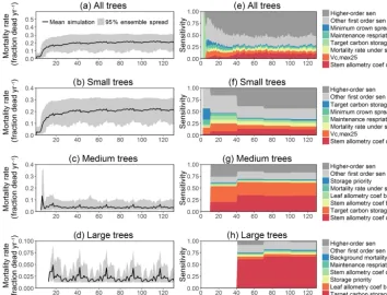
In this analysis, carbon starvation emerged as the main driver for tree mortality (Fig. D4). The carbon-starvation-based mortality uses a threshold of carbon storage to trigger mortality (see Appendix C). Under shaded conditions, lower carbon stores caused by the balance of NPP, respiration, and tissue growth/maintenance should lead to a higher mortality rate. As expected, the smaller tree size classes have much higher mortality rates (Fig. 4b–d). The first-order sensitiv-ity analysis of predicted mortalsensitiv-ity rate (percentage of mor-tality per year) shows that the dominant parameter for pre-dicting mortality of large trees is the target carbon storage (Fig. 4h); however, for small and medium trees, other param-eters such as allometric and photosynthetic paramparam-eters that could potentially determine their height growth and compet-itive advantages in the canopy are also important (Fig. 4f, g). Specifically, for medium-sized trees, the mortality rate is affected by both the stem allometry coefficient c and tar-geted carbon storage (Fig. 4g). For the small trees, impor-tant parameters include the photosynthetic capacity param-eter (Vc,max25), stem allometry coefficient c, mortality rate
under stress, and maintenance respiration, with the target car-bon storage having high sensitivity for small trees in the early years (Fig. 4f).
The simulated basal area (BA) of the forest, which is the total stem cross-sectional area per ground surface area, re-sults from the combination of both DBH growth and mortal-ity. The BA reaches equilibrium for different sizes of trees around year 70 (Fig. 5a). Our FAST analysis shows that a key parameter that controls BA in different tree size classes is the stem allometry coefficient c (Fig. 5e–h), which is a major parameter that determines the DBH growth (Fig. 2). We also found that the target carbon storage parameter that dominantly controls mortality is an important parameter for the simulated BA (Fig. 5e–h). Different from parameters im-portant for DBH growth at the individual tree level and mor-tality rate, a new parameter that becomes important for BA
of small and medium trees is the minimum crown spread, which determines the ratio of crown radius to DBH. A larger crown spread can lead to a smaller number of trees in the canopy and thus a lower BA (Fig. D5). The identified impor-tant parameters for the simulated tree density and fraction of trees are very similar to those identified for the simulated BA, except that the leaf allometry coefficientbbecomes very important for simulated small tree densities (Fig. 3e–h) and minimum height for fraction of trees (Fig. D6).
For the second-order sensitivity analysis, parametric in-teractions between stem allometry coefficientcand the pro-portion of carbon for seed allocation, and target carbon stor-age are found to be important for the prediction of total BA (Fig. D7). For trees of different sizes, parametric interactions between stem allometry coefficientc and minimum crown spread, target carbon storage, and maximum DBH are im-portant for small, medium, and large trees, respectively. For the prediction of dDBH and mortality, the contributions of most parametric interactions are relatively small except for large trees (Fig. D8). The interactions between stem allom-etry coefficientcand the proportion of carbon for seed allo-cation, maximum DBH, and stem allometry coefficientbare important for the prediction of dDBH for large trees. With respect to large tree mortality, the interaction between stem allometry coefficientcand target carbon storage is found to be important (Fig. D9).
3.2 Forest carbon cycles: carbon fluxes and stocks To investigate the key parametric control on carbon fluxes and stocks, we specifically investigate parameter sensitivi-ties for GPP, NPP, LAI, and total forest biomass. Our results show that GPP and NPP increased consistently for the first 10 years of the simulations, which is expected for a forest growing from bare ground (Fig. 6). However, within a fairly short period of 5–10 years, GPP, NPP, and LAI and their variance reached a quasi-stable rate. This amount of time to reach equilibrium is much shorter compared to the basal area (Fig. 6a) and the total biomass accumulations (Fig. 6d).
The first-order sensitivity analysis based on FAST shows that, for carbon fluxes of GPP and NPP, the photosynthetic capacity parameter (Vc,max25) is the most sensitive
Figure 4.Simulated temporal dynamics in tree mortality rates (fraction yr−1) and the corresponding first-order parametric sensitivity indices. The left panels show the mortality rate for(a)all,(b)small (diameter<10 cm),(c)medium (10 cm<diameter<50 cm), and(d)large trees (diameter>50 cm). Right panels show the sensitivity for the top six most important parameters for(e)all,(f)small,(g)medium, and(h)large trees, in order of importance. See Fig. 2 for details on legends.
for mortality especially for medium and large trees in the simulations (Fig. 4e–h), which account for a large proportion of total biomass (Fig. D11) and GPP (Fig. D12). This result supports hypothesis H3. For the second-order sensitivity, the contributions of most parametric interactions are relatively small (Fig. D13), as the first-order sensitivity accounts for a majority of the total variance in model outputs (Fig. 6e–h).
To understand how climate will impact sensitivity results, we also calculated the Spearman rank correlation coefficients between the first-order sensitivity index and the correspond-ing climate drivers. Our results show that the sensitivity of target carbon storage and maintenance respiration rate is neg-atively correlated with annual mean precipitation and relative humidity but is positively correlated with annual mean air temperature. This suggests that they are more important dur-ing the period of stressed conditions comprised of low pre-cipitation, low humidity, and high temperature (Fig. 7). Sen-sitivity to the leaf allometry coefficient b is positively cor-related with annual mean precipitation and relative humid-ity. This suggests the leaf carbon allocation is more impor-tant under favorable environmental conditions for growth. In general, our results suggests the climate has a larger impact on the parametric sensitivities for short-term carbon fluxes (GPP and NPP) and vegetation status (LAI) but has a smaller
impact on parametric sensitivities for long-term vegetation carbon stocks.
Our bivariate spline analysis (Wahba, 1990) shows that, forVc,max25and target storage carbon, an increase in either
of these parameters will cause an increase in the output of GPP, NPP, LAI, and biomass (Fig. 8). For the parameters re-lated to leaf and stem allometry, however, the relations may differ depending on the output and the year of interest. At year 130, the higher leaf allocation normally leads to higher fluxes (NPP and GPP) but less biomass. Meanwhile, higher stem allocation leads to higher biomass but smaller fluxes (NPP and GPP). This suggests that the trade-offs between carbon allocation to stem vs. leaf tissues leads to a corre-sponding trade-off between carbon stocks and productivity in the model predictions.
4 Discussion
sensi-Figure 5.Simulated temporal dynamics in basal area (BA, m2ha−1) and the corresponding first-order parametric sensitivity indices. The left panels show the simulated ranges of BA for(a)all,(b)small (diameter<10 cm),(c)medium (10 cm<diameter<50 cm), and(d)large trees (diameter>50 cm). Right panels show the sensitivity for the top six most important parameters for(e)all,(f)small,(g)medium, and
(h)large trees, in order of importance. See Fig. 2 for details on legends.
tivity analysis to determine the influential parameters over a specified region of the parameter space. So far, several uncer-tainty and sensitivity analyses have been conducted for size-structured land surface models (Pappas et al., 2013; LeBauer et al., 2013; Wang et al., 2013; Dietze et al., 2014; Collalti et al., 2019). In comparison with previous sensitivity anal-yses of size-structured models, our study considers a much larger number of parameters, i.e.,>80 compared with∼20– 35 parameters (Pappas et al., 2013; LeBauer et al., 2013; Wang et al., 2013; Dietze et al., 2014), the difference in para-metric sensitivity for different tree sizes, and the interactions among the key parameters. In general, our analysis shows similar results to sensitivity analysis on first-generation “big-leaf” vegetation models (e.g., Sargsyan et al., 2014), which show the importance of photosynthetic capacity,Vc,max25, for
predicting GPP and NPP. However, we do show important parameters that are unique to LSMs with second-generation vegetation demography. Specifically, results shown here in-dicate the importance of leaf and stem allometry parameters, which control dynamic carbon allocation strategies based on size, and thus control the general vegetative state and size structure of the forest (Waring et al., 1998; Waring and Run-ning, 2010). Importantly, a significant amount of variabil-ity in allometry is reported for different species and regions of the world (Feldpausch et al., 2011; Dietze et al., 2008),
the ranking of parameter importance changes with the size of plants (e.g., Fig. 2). This result is in agreement with a recent study that showed the influence of certain functional traits varied with size (Falster et al., 2018).
In our analysis, we observed a number of key similarities in model response to parameter variations in photosynthetic capacity, mortality, and respiration parameters (Pappas et al., 2013; LeBauer et al., 2013; Wang et al., 2013; Dietze et al., 2014); however, there are differences in the order of param-eter importance. For example, Dietze et al. (2014) showed that growth respiration fraction was the most important pa-rameter for the simulation of NPP, andVc,max25only ranked
as the seventh most important parameter. For our analysis, Vc,max25and growth respiration fraction are the first and
sec-ond most important parameters. This difference in parameter sensitivity rank may result from the fact that Dietze et al. (2014) used variable parameter ranges based on data (i.e., an uncertainty quantification study), while our sensitivity anal-ysis uses equal percentage variations (see details in the dis-cussion “limitation of methods” subsection). We also found that some parameters that are identified as important in other studies are not found to be important in our analysis. For ex-ample, Dietze et al. (2014) showed that water conductance that determines the upper boundary of transpiration is the second most important parameter for simulated NPP, but a similar parameter (smpso; Table D2) that defines soil water potential for opening stomata is not important in our analysis. This could be related to the fact that our site is much wetter than the temperate forests simulated by Dietze et al. (2014). Pappas et al. (2013) showed that the root distribution param-eter that dparam-etermines the fraction of fine roots in the upper soil layer is one of the top five parameters for the simulations of vegetation carbon fluxes and stocks; however, in our sensitiv-ity analysis, the two root distribution parameters (rootaand
rootb; Table D2) are not important for both vegetation
car-bon fluxes and stocks. This difference could also result from a wider range of variations (∼ ±30 %) in the study of Pappas et al. (2013) compared to our 15 % variations of the default parameters. Finally, our analysis shows the importance of al-lometry parameters, which are not considered in many previ-ous studies (Pappas et al., 2013; LeBauer et al., 2013; Wang et al., 2013; Dietze et al., 2014).
4.2 Comparing simulations with observations
The goal of our study is not to reproduce the observations but instead to identify important parameters that can be bet-ter estimated for the model to fit observations. Thus, we lay out potential parameter estimation improvements to achieve this goal. We do want to highlight three caveats. First, im-proved estimation of the most sensitive parameters may not be most efficient if they have relatively small uncertainty or variability across different species and locations. Second, even if the estimates for most sensitive parameters are per-fect, we may still not be able to fit model predictions to
ob-servations if there is deficiency in the representation of key processes in the model. Third, the recycled climate drivers from 1948 to 1972 may not match the observational periods. Given observation data limitations for our site, we conduct a qualitative comparison of our model simulations to ranges reported in the literature for the tropics. Not surprisingly, our model results show a variation of model–data mismatch for key vegetation states. For LAI (Fig. 6c), our simulated range is between∼1.9 and 6.0 m2m−2, which is lower than the observed range of∼3.0–6.9 m2m−2based on LAI esti-mated from MODIS (Knyazikhin et al., 1999) during 2000– 2016 within a 0.5◦window around our site. Our sensitivity analysis showed that leaf allometry coefficientb and target carbon storage are two key parameters for simulated LAI (Fig. 6g), and we expect that a better estimation of these parameters with data could potentially improve the model simulations. For GPP (Fig. 6a), the simulated range is be-tween∼1.0 and 3.0 kg C m−2yr−1, which is also lower than
the observed range of∼2.4–3.7 kg C m−2yr−1based on ex-trapolation from eddy flux tower observations and climate during 1981–2010 (Jung et al., 2009). Our analysis suggests that photosynthetic capacity, as represented byVc,max25,
tar-get carbon storage, and top-of-canopy specific leaf area, is an important parameter (Fig. 6a), and an improved estimation of them could help improve model simulations of GPP. We are not able to access on-site data for other model outputs. Therefore, we compare our model outputs with ranges from multiple tropical sites to evaluate their validity. For biomass (Fig. 6d), the simulated range of ∼2.5–12.5 kg C m−2 is lower than the observed range of∼7.3–21.3 kg C m−2from 21 transects within three tropical sites (Hunter et al., 2013). For BA (Fig. 5a), the simulated range of∼5.0–30.0 m2ha−1
is also lower than the observed range of∼17.1–35.2 m2ha−1
from five tropical sites (Hunter et al., 2013). Our results show that stem allometry coefficientcis the most important con-trol on BA and biomass, and an improved parameterization on stem allometry could help improve the model simula-tions. For the DBH growth, there are large variances in the observed values across different sites with the range of 0– 3 cm yr−1 (Lieberman et al., 1985; Worbes, 1999; Adams et al., 2014). The simulated average DBH growth is be-tween 0 and 0.4 cm yr−1but could be as high as 4 cm yr−1 for medium and large trees (Fig. 2). Based on our sensitiv-ity analysis (Fig. 2), we expected an improved parameteriza-tion of both allometry coefficientcand target carbon storage could help fit the model predictions to data.
Figure 6.Simulated temporal dynamics in carbon fluxes and stocks, and the corresponding first-order parametric sensitivity indices. The left panels show the simulated ranges for(a)GPP (kg C m−2yr−1),(b)NPP (kg C m−2yr−1),(c)LAI (m2m−2), and(d)total biomass (kg C m−2). Right panels show the sensitivity for the top six most important parameters for(e)all,(f)small,(g)medium, and(h)large trees, in order of importance. See Fig. 2 for details on legends.
0.5 %–5.7 % per year. However, for small and medium trees (Fig. 4b, c), the simulated mortality rate of∼15 %–30 % and ∼1 %–10 % is high when compared to the observed 95 % confidence interval of mortality rate of∼0.6 %–11.3 % and ∼0.8 %–3.0 % for small and medium trees, respectively. The high predicted mortality rate of small trees could result from the fact that the model predicts a very high mortality rate for very small trees (<1 cm), as they cannot survive after es-tablishment due to low light conditions in the simulations. Since the small trees have such a large fraction of the pop-ulation in our simpop-ulations (Fig. 3b), the overall mortality rate (Fig. 4a) of ∼15 %–30 % is also high when compared to observations (∼0.6 %–11.3 %); however, if we separate the mortality rate of very small trees from the calculation of the overall mortality, then the simulated mortality rates of 1 %–10 % (Fig. D14b) are in the range of observations. The very high mortality rate range of smaller trees (∼10 %– 30 %; Fig. D14a) spans the reported seedling/sapling mor-tality rate, e.g., ∼15 %–21 % per year from 1- to 20-year-old tropical forest stands in Costa Rica (Dupuy and Chaz-don, 2006). However, there is potential for improvement for site-level simulations as the current recruitment algorithm within CLM4.5(FATES) depends only on the availability of seed bank but not on the density, light, and water availability. The relatively high mortality rate of small and medium trees
could also be linked to the fact that CLM4.5(FATES) uses the perfect plasticity approximation (PPA) to simulate the canopy light availability for understory trees (Fisher et al., 2018), which may create canopy closure too fast for the small- and medium-sized trees to survive under low light conditions. We expect that future improvements in recruit-ment and representation of the light environrecruit-ment within the PPA could be helpful for a better prediction of tree mortality for small- and medium-sized trees. It is also possible that the observed mortality rate for small trees could potentially be underestimated if all the trees in a certain size classes died at a shorter time frame than the census intervals. Our sensitiv-ity analysis indicates that key model parameters that can be better estimated for improved mortality predictions include stem allometry parameters,Vc,max25, target carbon storage,
and mortality rate under stress (Fig. 4).
Figure 7.Spearman’s correlation coefficients between climate drivers and six most important parameters identified for(a)GPP,(b)NPP,
(c)LAI, and(d)biomass.
traits into the model is to represent the trait trade-off and co-ordination for different PFTs. Through our sensitivity analy-sis, we have identified key parameters for vegetation dynam-ics, which can be targeted for the representation of trait trade-off and coordination in the tropics. For example, our study shows that a higher stem carbon allocation could reduce the GPP and a higherVc,max25could increase GPP (Fig. 8). The
potential exploration of trade-off and coordination between these two parameters could be critical to resolve different PFTs and represent the trait variations. Even though the sim-ulated ranges of the model outputs are different than the ob-servations, our sensitivity analysis should still be valid in view that a primary end goal of this research is to identify im-portant parameters that can be better estimated for the model to better fit observations. For example, Holm et al. (2019) uti-lized results from our study to implement their tropical forest parameterization, specifically by increasing their target car-bon storage parameter to obtain higher survival and lower growth.
In addition to directly comparing the model outputs to ob-servations, we want to highlight that the sensitivity analysis will also allow us to explore the functional relationships be-tween model parameters and outputs. Future synthesis stud-ies that show these functional relationships using data across different sites could be very useful to evaluate the fidelity of
model structure to represent the key processes that control these relationships.
4.3 Limitation of methods
Our study is the first global sensitivity analysis for CLM4.5(FATES); however, it is subjected to several limi-tations that could be improved for future studies. First, our study uses an arbitrary choice of parameter ranges (±15 %), which determines the variance in the model outputs and the corresponding results of the sensitivity analysis. However, we expect that our analysis can reveal the importance of parameters given equal percentage of variations, which can help us gain a better understanding of the model structure. We do acknowledge that uncertainty analysis studies that specifically consider the potential ranges of values in trop-ical forests based on observations could provide insights on which additional measurements are needed to explain vari-ance in the model prediction.
Figure 8.Relations between outputs of CLM4.5(FATES), including GPP, NPP, LAI, and biomass (units shown in Fig. 6), and the most sensitive parameters, i.e.,Vc,max25(units are µmol CO2m−2s−1), target storage carbon (unit is the ratio of leaf biomass), leaf and stem
allocation (unitless parameters) for simulation year 10 (red) and 130 (blue). Shown are the mean relations with the 95 % confidence intervals in grey envelopes. These figures show how an output will generally increase or decrease when a given parameter is changed.
model output ranges and the sensitivity results. However, our exploration of parameter sensitivity assuming their indepen-dence could still help us understand the baseline parameter control on model behaviors (Xu and Gertner, 2009). The exploration of trade-offs and coordination among different parameters requires data analysis for multiple traits of the same species. The Predictive Ecosystem Analyzer (PEcAn) framework (LeBauer et al., 2013) could be a useful tool to synthesize plant trait data to estimate model parameter dis-tributions. The challenge is that, even though there are great efforts in the research community to compile plant trait data across the globe (Kattge et al., 2011a, b), there are still lim-ited datasets with observations of multiple traits for the same species. Future uncertainty analysis studies that explicitly consider the prior distributions and correlations for all the pa-rameters can build on this analysis and gain further insights on where the uncertainty in the model predictions comes from.
Third, it is possible that the parameter sensitivity could be different if we use different model inputs, different sites, and different structures of subcomponents within the model. For example, using site-level climate drivers, instead of the reanalysis meteorological drivers used in this study (Qian et al., 2006), could lead to different sensitivity values since our analysis showed that parameter importance is quite sen-sitive to different climate conditions. Furthermore, there are
ongoing development activities to improve different com-ponents of the models. For example, there are current ef-forts to incorporate different representations of tree allom-etry within CLM4.5(FATES), which have different formula-tions between size and biomass, e.g., Chave et al. (2014), or the current formulation of the photosynthetic process in the CLM4.5(FATES) can be replaced with a model that more accurately represents the allocation of nitrogen and thus the photosynthetic process (see Xu et al., 2013; Ali et al., 2016). Therefore, model improvements such as these can affect cor-responding sensitivity analysis results. To understand the im-pact of site-level variations on model dynamics, similar sen-sitivity analysis across different sites can be conducted to understand how climate variability will affect the sensitivity analysis results.
5 Conclusions
LSMs have many parameters that could potentially affect the outcome of their simulations. In this study, we use the FAST analysis to conduct a high-dimensional global sensi-tivity analysis on CLM4.5(FATES). We use an intermediate complexity of simulation: runs are sufficiently long to per-mit short-term physiological variance to propagate into the long-term forest demographic structure. Even though we do not explore competitive dynamics between different PFTs, our sensitivity analysis will guide us on the selection of key plant traits for the consideration of trait trade-off and coordination in order to improve PFT coexistence within CLM4.5(FATES).
Our analyses show that the target carbon storage and stem allometry parameters are important for the simulation of DBH growth for individual trees and tree mortality. The pho-tosynthetic parameter,Vc,max25, is the most important for the
simulation of carbon fluxes including GPP and NPP. The combination of stem allometry, target carbon storage, and Vc,max25 dominantly control the simulation of total BA and
long-term carbon stocks. These identified growth and sur-vival parameters will help us better understand the key con-trol of fast and slow carbon and vegetation dynamics within the next generation of demographically enabled LSMs to-ward improved model parameterization and model structure. The results of the sensitivity analysis presented here can be utilized to construct the parameter-output response sur-face for the CLM4.5(FATES) model, which can assist fu-ture efforts for model calibration or diagnosis. These find-ings may help us better understand the overall model struc-ture and guide the estimation of key model parameters with significant control over vegetative processes in these models for better model fitting to data. The FAST analysis provides a promising means of analyzing complex LSM components and can be a powerful tool in understanding the necessar-ily high-dimensional representation of living systems within Earth system models.
Code and data availability. To access the FATES source code,
Appendix A: Allometry equations
The following equations are cohort-based calculations for al-lometry in CLM4.5(FATES). Interested readers are referred to Fisher et al. (2015) for more information. The parameters used for the allometry equations include dbh2hm, dbh2hc,
dbh2bda, dbh2bdb, dbh2bdc, and dbh2bdd (all are unitless
variables). Specifically, the dead wood biomass (BD; kg C) is calculated as a function of diameter (DBH; cm), height (h; meter), and wood density (g cm−3):
BD=(dbh2bda)(hdbh2bdb)(DBHdbh2bdc)(densitydbh2bdwood d).
(A1) The height (m) is calculated based on DBH (cm) as fol-lows:
H=10dbh2hc(DBHdbh2bdm). (A2)
Appendix B: Temperature response curve
The parameters used for the temperature response curve equations include the equation to calculate the maximum car-boxylation rate, Vc,max25, the maximum electron transport
rate, Jmax, and the triose phosphate use (TPU) limited
car-boxylation rate, TPU (also all parameters here are unitless) (Fisher et al., 2015). The temperature response equations for Vc,max,z,Jmax,z, and TPUzare
Vc,max,z=Vc,max,25(e
vcmaxha
(0.001rgas)(tfrz+25))(1−tfrz+25 tveg
)
( vcmaxc
1+e−vcmaxhd+(vcmaxse)(tveg)) (B1)
Jmax,z=Jmax,25(e
jmaxha
(0.001rgas)(tfrz+25))(1−tfrz+25 tveg
)
( jmaxc
1+e−jmaxhd+(jmaxse)(tveg)) (B2)
TPUz=tpu25(e
tpuha
(0.001rgas)(tfrz+25))(1−tfrz+25 tveg
)
( tpuc
1+e−tpuhd+(tpuse)(tveg)), (B3)
wheretfrzis the freezing point of water in Kelvin (273.15 K).
Appendix C: Carbon storage in CLM4.5(FATES) The target carbon storage is the cushion parameter shown in Table D3. Specifically, a higher value of this parameter will lead to a higher allocation of carbon to storage and thus a lower allocation to growth at the specific time step. Also, carbon storage plays an important role for the simulated mor-tality through the parameter that controls the mormor-tality rate under stress, stress_mort in Table D3. The tree will be un-der stress when it has low carbon storage (<leaf biomass).
Therefore, the target carbon storage parameter and the mor-tality rate under stress parameter play a large role in deter-mining the level of mortality that occurs in the simulations.
Carbon storage,bstore (in kg C/cohort), plays a very
im-portant role in both growth and mortality (Fisher et al., 2015). Specifically, CLM4.5(FATES) assumes a target car-bon storage determined by the multiplication of leaf biomass (bleaf) and the target carbon storage parameter (i.e., the
tar-get amount of carbon plants store relative to leaf biomass; Scushion, variable cushion in Table D3). At the specific time,
the carbon balance for growth and storage is calculated as follows:
C=NPP−Tmdfmd,min, (C1)
whereTmdis the maintenance respiration andfmd,minis the
minimum fraction of the maintenance demand (storage pri-ority parameter in Table D1) that the plant must meet each time step, which represents a life-history-strategy decision concerning whether leaves should remain on in the case of low carbon uptake (a risky strategy) or not be replaced (a conservative strategy).
The fraction of the carbon balance for each cohort allo-cated to the carbon storage pool (fstore) will be determined
by the following equations: fstore=e(−ftstore)
4
, (C2)
where
ftstore=max 0,
bstore Scushionbleaf
. (C3)
Thus, the target carbon storage parameter,Scushion, can
af-fect carbon allocations. Specifically, a higher value ofScushion
will lead to a higher allocation of carbon to storage and thus lower allocation to growth at the specific time step.
Carbon storage also plays an important role for the mor-tality. Specifically, carbon starvation mortality (Mcs) is
cal-culated as follows: Mcs=Smmax 0,1−
bstore bleaf
, (C4)
whereSm is the stress mortality factor (i.e., stress_mort in
Appendix D: Appendix figures and tables
Figure D1.Comparison of first-order parametric sensitivity for medium (10 cm<diameter<50 cm) tree density averaged over 20, 30, and 40 years.
Figure D3.Impacts of stem allometry on the change in diameter at breast height (dDBH) averaged over the simulation years 100–130 for trees of different sizes. The shaded area shows the 95 % confidence interval of these relations.
Figure D5.Impacts of minimum crown spread on the basal area (BA) averaged over the simulation years 100–130 for trees of different sizes. The shaded area shows the 95 % confidence interval of these relations.
Figure D7.Second-order sensitivity index of the model parameters for the basal area (BA) outputs from CLM4.5(FATES) for(a)all trees,
(b)small trees,(c)medium trees, and(d)large trees. Shown are the top eight most important parameter interactions in order of importance based on the mean parametric sensitivity across years (red is the most important and blue is the least important)
Figure D9.Second-order sensitivity index of the model parameters for the mortality outputs from CLM4.5(FATES) for(a)all trees,(b)small trees,(c)medium trees, and(d)large trees. Shown are the top eight most important parameter interactions in order of importance based on the mean parametric sensitivity across years (red is the most important and blue is the least important).
Figure D11.Fraction of total biomass for trees of different sizes, including small (diameter<10 cm), medium (10 cm<diameter<50 cm), and large trees (diameter>50 cm).
Figure D13.Second-order sensitivity index of the model parameters for the GPP, NPP, LAI, and biomass outputs from CLM4.5(FATES). Shown are the top eight most important parameter interactions in order of importance based on the mean parametric sensitivity across years (red is the most important and blue is the least important).
Table D1.Parameter sets used in this study – part 1.
Name Variable name Units Default Lower Upper
Allocation and allometry parameters
Height allometry coefficientm dbh2hm (–) 0.64 0.54 0.74
Height allometry coefficientc dbh2hc (–) 0.37 0.31 0.43
Leaf allometry coefficienta dbh2bla (–) 0.042 0.036 0.048
Leaf allometry coefficientb dbh2blb (–) 1.56 1.33 1.79 Leaf allometry coefficientc dbh2blc (–) 0.55 0.47 0.63
Leaf allometry SLA scaler dbh2bl_slascaler (–) 0.03 0.025 0.035 Stem allometry coefficienta dbh2bda (–) 0.069 0.059 0.079
Stem allometry coefficientb dbh2bdb (–) 0.57 0.49 0.66
Stem allometry coefficientc dbh2bdc (–) 1.94 1.65 2.23
Stem allometry coefficientd dbh2bdd (–) 0.93 0.79 1.07
SAI scaler SAI scaler (–) 0.05 0.043 0.058 Ratio of sapwood to leaf area sapwood-ratio (m−1) 0.001 0.00085 0.00115 Fraction of root to leaf biomass froot_leaf (g C g C−1) 1 0.85 1.15 Seed allocation seed_alloc (0–1) 0.1 0.085 0.115 Fraction of aboveground stem ag_biomass (0–1) 0.6 0.51 0.69 Crown depth crown (0–1) 0.5 0.43 0.58 Maximum crown spread max spread (cm m−2) 0.3 0.25 0.35 Minimum crown spread min spread (cm m−2) 0.18 0.15 0.21 Root distribution coefficienta roota (m−1) 7 5.95 8.05
Root distribution coefficientb rootb (m−1) 1 0.85 1.15
Table D2.Parameter sets used in this study – part 2.
Name Variable name Units Default Lower Upper
Regrowth parameters
Initial seedling density initd (m−2) 0.8 0.68 0.92 Seed rain seed_rain (kg C m−2yr−1) 0.28 0.24 0.32
Minimum height hgt_min (m) 1.25 1.06 1.44
Photosynthetic and respiration parameters
Stomata conductance slope bb_slope (–) 9 7.65 10.35
Vc,max25 fnitr (µmol CO2m−2s−1) 60 51 69
Leaf C:N leafcn (g C g N−1) 30 25.5 34.5 Storage priority leaf_stor_priority (0–1) 0.8 0.68 0.92 Top-of-canopy SLA slatop (m2g C−1) 0.012 0.010 0.014 Growth respiration fraction grperc (–) 0.3 0.26 0.34 Maintenance respiration lmr25top (µmol CO2m−2s−1) 0.71 0.60 0.82
Soil water potential for stomata closure smpso (mm) −2.55×10⁴ −2.93×10⁴ −2.16×10⁴ Soil water potential for opening stomata smpso (mm) −6.60×10⁴ −7.59×10⁴ −5.61×10⁴
Temperature response parameters
Vc,maxtemperature coefficient ha vcmaxha (–) 6.53×10⁴ 5.55×10⁴ 7.51×10⁴ Jmaxtemperature coefficient ha jmaxha (–) 4.35×10⁴ 3.70×10⁴ 5.00×10⁴
TPU temperature coefficient ha tpuha (–) 5.31×10⁴ 4.51×10⁴ 6.10×10⁴ Maintenance respiration coefficient ha lmrha (–) 4.63×10⁴ 3.94×10⁴ 5.33×10⁴ Vc,maxtemperature coefficient hd vcmaxhd (–) 14.92×10⁴ 12.68×10⁴ 17.16×10⁴ Jmaxtemperature coefficient hd jmaxhd (–) 15.20×10⁴ 12.92×10⁴ 17.48×10⁴
TPU temperature coefficient hd tpuhd (–) 15.06×10⁴ 12.80×10⁴ 17.32×10⁴ Maintenance respiration coefficient hd lmrhd (–) 15.06×10⁴ 12.80×10⁴ 17.32×10⁴ Vc,maxtemperature coefficient se vcmaxse (–) 485 412 558 Jmaxtemperature coefficient se jmaxse (–) 495 420 570
Table D3.Parameter sets used in this study – part 3.
Name Variable name Units Default Lower Upper
Mortality parameters
Background mortality b_mort (yr−1) 0.014 0.012 0.016 Target carbon storage cushion ratio of leaf biomass 1.2 1.02 1.38 Mortality rate under stress stress_mort (yr−1) 0.6 0.51 0.69 Understory mortality rate understory_death (–) 0.56 0.48 0.64 Seed mortality rate sd_mort (yr−1) 0.98 0.83 1.0 Hydraulic failure threshold hf_sm_threshold (–) 1.00×10⁻⁶ 8.5×10⁻⁷ 1.15×10⁻⁶ Turnover parameters
Leaf longevity leaf_long (years) 1.5 1.28 1.72 Root longevity root_long (years) 1 0.85 1.15 Stem Turnover alpha_stem (years) 0.01 0.0085 0.0115
Radiation parameters
Leaf reflectance: near IR rholnir (0–1) 0.45 0.38 0.52 Leaf reflectance: visible rholvis (0–1) 0.1 0.085 0.115 Stem reflectance: near IR rhosnir (0–1) 0.39 0.33 0.45 Stem reflectance: visible rhosvis (0–1) 0.16 0.14 0.18 Leaf transmittance: near IR taulnir (0–1) 0.25 0.21 0.29 Leaf transmittance: visible taulvis (0–1) 0.05 0.043 0.058 Stem transmittance: near IR tausnir (0–1) 1.00×10⁻³ 8.5×10⁻⁴ 1.15×10⁻³ Stem transmittance: visible tausvis (0–1) 1.00×10⁻³ 8.5×10⁻⁴ 1.15×10⁻³ Leaf orientation index xl (−0.4<xl<0.6) 0.1 0.085 0.115
Competition parameters
Table D4.Parameter sets used in this study – part 4.
Name Variable name Units Default Lower Upper
Phenology parameters
Drought deciduous threshold ed_phdrought−threshold (0–1) 0.15 0.13 0.17
Phenology coefficienta ed_pha (–) −68 −78.2 −57.8
Phenology coefficientb ed_phb (–) 638 542.3 733.7
Phenology coefficientc ed_phc (–) −1.00×10⁻³ −1.15×10⁻³ −8.5×10⁻⁴
Chilling day temperature ed_phchiltemp ◦C 5 4.25 5.75
Cold day temperature ed_phcoldtemp ◦C 7.5 6.4 8.6
Cold days for leaf drop-off ed_phncolddayslim days 5 4.3 5.8 Minimum days before leaf on ed_phmindayson days 30 25 35
Minimum days before leaf drops ed_phdoff−time days 100 85 115
Seed turnover seed_turnover (yr−1) 0.51 0.43 0.59 Germination rate germination_timescale (yr−1) 0.5 0.43 0.58 Aerodynamic parameters
Leaf dimension dleaf (m) 0.04 0.034 0.046
Momentum roughness length z0mr (–) 0.075 0.064 0.086 Displacement height ratio displar (m) 0.67 0.57 0.77
Additional parameters
Author contributions. All authors contributed to the manuscript writing. CX designed the numerical experiments, developed scripts for sensitivity analysis, and analyzed model results; ECM imple-mented the model runs, extracted the model outputs, and analyzed model results; RAF, RGK, CDK, CX, and BOC contributed to the model development and simulations; JAH, DMR, SPS, and APW provided suggestions on sensitivity analysis, and LW provided sup-port for model simulations; DJJ provide data on model evaluations; NGM, LMK, JQC, and JAV provided support and guidance on the experiment and manuscript.
Competing interests. The authors declare that they have no conflict
of interest.
Acknowledgements. Model simulations were made possible thanks
to the Conejo supercomputing system at the Los Alamos National Laboratory (LANL). We thank the four reviewers for their very helpful comments that substantially improved our manuscript.
Financial support. This work was supported by the United States
Department of Energy (US DOE) Office of Science Next Gen-eration Ecosystem Experiment at Tropics (NGEE-T) project, the DOE Graduate Student Researcher (SCGSR) Fellowship, and the UC-Lab Fees Research Program (grant nos. 237285 and LFR-18-542511). Shawn P. Serbin was also partially supported by the United States Department of Energy contract no. DE-SC0012704 to Brookhaven National Laboratory. A portion of Elias C. Mas-soud’s contribution to this research was carried out at the Jet Propul-sion Laboratory, California Institute of Technology, under a contract with the National Aeronautics and Space Administration, Copyright 2019.
Review statement. This paper was edited by Christoph Müller and
reviewed by Xiangtao Xu, Nancy Kiang, and Sebastian Lienert.
References
Adams, H. R., Barnard, H. R., and Loomis, A. K.: Topography alters tree growth–climate relationships in a semi-arid forested catch-ment, Ecosphere, 5, 1–16, 2014.
Ali, A. A., Xu, C., Rogers, A., Fisher, R. A., Wullschleger, S. D., Massoud, E. C., Vrugt, J. A., Muss, J. D., McDowell, N. G., Fisher, J. B., Reich, P. B., and Wilson, C. J.: A global scale mechanistic model of photosynthetic capacity (LUNA V1.0), Geosci. Model Dev., 9, 587–606, https://doi.org/10.5194/gmd-9-587-2016, 2016.
Archer, G., Saltelli, A., and Sobol,I.: Sensitivity measures, anova-like techniques and the use of bootstrap, J. Stat. Comput. Simu., 58, 99–120,1997.
Arora, V. K., Boer, G. J., Friedlingstein, P., Eby, M., Jones, C. D., Christian, J. R., Bonan, G., Bopp, L., Brovkin, V., Cadule, P., Brovkin, V., Cadule, P., and Hajima, T.: Carbon–concentration
and carbon–climate feedbacks in cmip5 earth system models, J. Climate, 26 5289–5314, 2013.
Bastidas, L. A., Gupta, H. V., Sorooshian, S., Shuttleworth, W. J., and Yang, Z. L.: Sensitivity analysis of a land surface scheme us-ing multicriteria methods, J. Geophys. Res.-Atmos., 104, 19481– 19490, 1999.
Benton, T. G. and Grant, A.: Elasticity analysis as an important tool in evolutionary and population ecology Trends Ecol. Evol., 14, 467–471, 1999.
Bonan, G. B., Lawrence, P. J., Oleson, K. W., Levis, S., Jung, M., Reichstein, M., Lawrence, D. M., and Swenson, S. C.: Im-proving canopy processes in the community land model ver-sion 4 (CLM4) using global flux fields empirically inferred from fluxnet data, J. Geophys. Res.-Biogeo., 116, G02014, https://doi.org/10.1029/2010JG001593, 2011.
Campolongo, F., Saltelli, A., Sørensen, T. M., and Tarantola, S.: Hitchhiker’s guide to sensitivity analysis, in: Sensitivity analysis, IEEE Computer Society Press, 15–47, 2000.
Chave, J., Réjou-Méchain, M., Búrquez, A., Chidumayo, E., Col-gan, M. S., Delitti, W. B., Duque, A., Eid, T., Fearnside, P. M., Goodman, R. C., and Henry, M.: Improved allometric mod-els to estimate the aboveground biomass of tropical trees, Glob. Change Biol., 20, 3177–3190, 2014.
Christoffersen, B. O., Gloor, M., Fauset, S., Fyllas, N. M., Gal-braith, D. R., Baker, T. R., Kruijt, B., Rowland, L., Fisher, R. A., Binks, O. J., Sevanto, S., Xu, C., Jansen, S., Choat, B., Men-cuccini, M., McDowell, N. G., and Meir, P.: Linking hydraulic traits to tropical forest function in a size-structured and trait-driven model (TFS v.1-Hydro), Geosci. Model Dev., 9, 4227– 4255, https://doi.org/10.5194/gmd-9-4227-2016, 2016.
Claussen, M., Mysak, L., Weaver, A., Crucifix, M., Fichefet, T., Loutre, M. F., Weber, S., Alcamo, J., Alexeev, V., Berger, A., and Calov, R.: Earth system models of intermediate complexity: closing the gap in the spectrum of climate system models, Clim. Dynam., 18, 579–586, 2002.
Collalti, A., Thornton, P. E., Cescatti, A., Rita, A., Borghetti, M., Nole, A., Trotta, C., Ciais, P., and Matteucci, G.: The sensitivity of the forest carbon budget shifts across processes along with stand development and climate change, Ecol. Appl., 29, e01837, https://doi.org/10.1002/eap.1837, 2019.
Collins, D. C. and Avissar, R.: An evaluation with the fourier am-plitude sensitivity test (FAST) of which land-surface parameters are of greatest importance in atmospheric modeling, J. Climate, 7, 681–703, 1994.
Cox, P. M., Betts, R. A., Jones, C. D., Spall, S. A., and Totterdell, I. J.: Acceleration of global warming due to carbon-cycle feed-backs in a coupled climate model, Nature, 408, 184–187, 2000. Crossley, J. F., Polcher, J., Cox, P. M., Gedney, N. and Planton, S.:
Uncertainties linked to land-surface processes in climate change simulations, Clim. Dynam., 16, 949–961, 2000.
Cukier, R., Fortuin, C., Shuler, K. E., Petschek, A., and Schaibly, J.: Study of the sensitivity of coupled reaction systems to uncertain-ties in rate coefficients. I theory, J. Chem. Phys., 59, 3873–3878, 1973.