Dynamic interaction between shear bands

(1)

Curriculum 3. Modelling and Simulation

Diana Giarola

Dynamic interaction between

shear bands

Doctoral School in Civil, Environmental and Mechanical Engineering

(2)

University of Trento

Doctoral Thesis

Dynamic interaction between shear

bands

Author:

Diana Giarola Prof. Davide BigoniSupervisor: Prof. Andrea Piccolroaz Dott. Domenico Capuani

Topic 3. Modelling and Simulation XXXI cycle 2015/2018

(3)

Except where otherwise noted, contents on this book are licensed under a Creative Common Attribution - Non Commercial - No Derivatives

4.0 International License University of Trento

Doctoral School in Civil, Environmental and Mechanical Engineering http://web.unitn.it/en/dricam

Via Mesiano 77, I-38123 Trento

(4)

UNIVERSITY OF TRENTO Graduate School in Structural Engineering Modelling and Simulation XXXI Cycle

Ph.D. Program Head: prof. D. Bigoni

Final Examination: 28 March 2019

(5)

(6)

Abstract

A shear band of nite length, formed inside a ductile material at a cer-tain stage of a continued homogeneous strain, provides a dynamic per-turbation to an incident wave eld, which strongly inuences the dy-namics of the material and aects its path to failure. The investigation of this perturbation is presented for a ductile metal, with reference to the incremental mechanics of a material obeying theJ2-deformation the-ory of plasticity (a special form of prestressed, elastic, anisotropic, and incompressible solid). The treatment originates from the derivation of integral representations relating the incremental mechanical elds at ev-ery point of the medium to the incremental displacement jump across the shear band faces, generated by an impinging wave. The boundary integral equations (under the plane strain assumption) are numerically approached through a collocation technique, which takes account of the singularity at the shear band tips and permits the analysis of an incident wave impinging on a shear band.

It is shown that the presence of the shear band induces a resonance, visi-ble in the incremental displacement eld and in the stress intensity factor at the shear band tips, which promotes shear band growth. Moreover, the waves scattered by the shear band are shown to generate a ne tex-ture of vibrations, parallel to the shear band line and propagating at a long distance from it, but leaving a sort of conical shadow zone, which emanates from the tips of the shear band.

(7)

(8)

Acknowledgements

Firstly, I would like to thank Professor Davide Bigoni for the great op-portunity, the motivation and the encouragements that he gave me in these three years. I am also deeply grateful to Dr. Domenico Capuani for the help and the support despite the great distance, and our super productive meetings from Ferrara to Bologna.

Moreover, I would like to thank all members of the Solid and Structural Mechanics Group at the University of Trento, and in particular the col-leagues of "Aula Prof. Bacca" and the Instabilities Lab. Last but not the least, I would like to thank my family and my friends for their constant support during these years.

(9)

(10)

List of pubblications

The results reported in the present thesis have been summarized in the following papers:

• D. Bigoni, D. Capuani, D. Giarola (2017). Dynamics of shear bands

in a prestressed material. Conference proceeding of the 21st Inter-national Conference on Composite Materials.

• D. Giarola, D. Capuani, D. Bigoni (2018). The dynamics of a shear

band. Journal of the Mechanics and Physics of Solids 112, 472-490.

• D. Giarola, D. Capuani, D. Bigoni (2018). Dynamic interaction of

multiple shear bands. Scientic Reports 8:16033.

• D. Bigoni, D. Capuani, D. Giarola (2019). Scattering of waves

(11)

(12)

1 Introduction

When a ductile material is subject to severe strain, failure is preluded by the emergence of shear bands which initially nucleate in a small area, but quickly extend rectilinearly and accumulate damage, until they de-generate into fractures. Nucleation and growth of shear bands and their interactions in ductile materials are concurrent causes of failure, a com-plex process which is strongly aected by dynamics and far from being completely understood. Therefore, research on shear bands yields a fun-damental understanding of the intimate rules of failure, so that it may be important in the design of new materials with superior mechanical performances.

The aim of the present thesis is to investigate dynamic perturbations in the stress/deformation elds of an incident wave, induced by multiple shear bands interaction, formed inside a ductile metal, at a certain stage of a continued strain.

The incremental constitutive equations used to describe nonlinear ma-terials are briey introduced in Chapter 2 together with the condition for their positive deniteness, ellipticity, and regime classication, in the spe-cial cases of the J2-deformation theory of plasticity and Mooney-Rivlin material.

(17)

Chapter 1. Introduction

for the incremental nonlinear elasticity. In order to give a numerical solution to the shear band problem, a Boundary Element Method with an ad hoc collocation technique is formulated.

The case pertaining to an isolated shear band in innite incompress-ible nonlinear elastic material is reported in Chapter 5. Displacements, Stress Intensity Factors, and deviatoric strain elds are presented for the cases of a time-harmonic transverse shear wave that travels orthogonal to the shear band, and with generic inclination with respect to it. Results show that wave propagation induces a resonance eect of the shear band, promoting its growth, and show that the scattered eld of a shear band is composed by a family of plane waves parallel to the band, Figure 1.1.

4

-4 0 8

-8

4

-4 0 8

-8

0 4 8

-4

-8 -8 -4 0 4 8

x l1/ x l1/

x l2/ x l2/

0 4 8

-4

-8 -8 -4 0 4 8

x l1/ x l1/

Figure 1.1: Scattered (left) and total (right) incremental deviatoric strain eld is reported as produced by an incident shear wave travelling parallel to the shear band of length2l(β=θ, withβ direction of the wave propagation andθ inclination of the shear band) with wave numberΩl/c1 = 1 (denoting withΩ the circular frequency andc1 the wave speed).

The dynamic interaction of multiple shear bands is introduced in Chapter 6, where the appropriate numerical technique used to solve the problem is described in detail. Four dierent congurations of shear bands are considered in Chapter 7: parallel and aligned shear bands, two

(18)

Chapter 1. Introduction

shear bands in a V-shaped conguration and four shear bands in a squared conguration. Results show that dierent geometries of shear bands can lead to opposite eects, of focusing or shielding from waves (Figure 1.2), and in some cases promote resonance eects or the annihilation of the shear band.

0 -2

-4 2 4

-2

-4 2

0 -2

-4 2 4

x2/_l 0

-2

-4 2

0 -2

-4 2 4 -4 -2 0 2 4

x1/_l

x2/_l

x1/_l

x1/_l x1/_l 0

-2

-4 2 0

-2

-4 2

0

x2/_l

(19)

(20)

2 The incremental constitutive

equations for incompressible plane

strain

In this Chapter, the set of equations that characterise the problem of the incremental nonlinear elasticity upon which the present thesis is focussed, is briey illustrated. The analysis of strain localizations, in the form of shear bands, can be only analyzed by the using of the incremental elasticity due to the large strains involved.

To this purpose, the Biot problem [10] has been chosen, in which an innite medium is homogeneously and biaxially deformed within the ellip-tic range. The current conguration is plane strain and characterized by two in-plane stretches. The incremental response of this incompressible solid is linear and governed by the two Biot moduli, which are functions of the in-plane stretches.

2.1 The incremental constitutive equation

(21)

Chapter 2. The incremental constitutive equations for incompressible plane strain

Cauchy-Green left tensor B=FFT, as

σ =−qI+β0B+β1B−1, (2.1)

in which q is function of the hydrostatic pressure pˆ = trσ/3 with the

relation

q =−pˆ+1

3β0I1+

1

6β1 I

2 1 −I2

, I1= trB, I2= trB2, (2.2)

and β0 andβ1 are generic functions of the two invariants (I1, I2) ofB

β0=β0(I1, I2), β1 =β1(I1, I2). (2.3)

The constitutive equation (2.1) implies the coaxiality between tensorsB

and σ, so that they share a principal reference system where

diagB= (λ2₁, λ2₂, λ₃2), diagσ= (σ1, σ2, σ3), (2.4)

in whichσiare the principal stresses andλi>0are the principal stretches

that satisfy the incompressibility constraint

λ1λ2λ3 = 1. (2.5)

Consequently, terms β0 and β1 of equation (2.1) can be determined in the principal Eulerian reference system as follows

β0 = 1

λ2 1−λ22

(σ1−σ3)λ2₁ λ2

1−λ33

−(σ2−σ3)λ

2 2 λ2

2−λ23

(2.6)

and

β1 =

1

λ2₁−λ2₂

σ1−σ3 λ2₁−λ3₃ −

σ2−σ3 λ2₂−λ2₃

(2.7)

Biot [10] has shown that the most general incremental response of a hyperelastic incompressible material deformed in plane strain can be characterized in terms of the Zaremba-Jaumann derivative of the Cauchy stress ∇σ,

∇

σ= ˙σ−Wσ+σW, (2.8)

(22)

2.1. The incremental constitutive equation

(where W is the incremental rotation tensor and σ˙ is the increment of

Cauchy stress) as

∇ σ11−

∇

σ22= 2µ∗(D11−D22), ∇σ12= 2µD12, (2.9)

where, in an updated Lagrangean description (in which the current state is used as reference), Dij are the in-plane components of the Eulerian

strain increment tensor D, which has to satisfy the incompressibility

constraint trD = 0, and µ and µ∗ are two incremental shear moduli, respectively parallel and inclined at 45◦ _{with respect to the} _x1₋_{axis [}₄_], and they can be expressed as functions of the principal stretches

µ= λ

2 1+λ22

2

β0− β1

λ2 1λ22

. (2.10)

and

µ∗ = λ

2 1+λ22

2 β0+

λ2₁−λ2₂

4

λ2₁∂β0 ∂λ1 −λ

2 2 ∂β0 ∂λ2 − 1 λ2 1λ22

λ2 1+λ22

2 β1+

λ2 1−λ22

4

λ2₁∂β1 ∂λ1 −λ

2 2 ∂β1 ∂λ2 (2.11)

In terms of the unsymmetric nominal stress increment _t˙_{, related to}

the Zaremba-Jaumann derivative of the Cauchy stress as

˙

t=σ∇−σW−Dσ, (2.12)

the constitutive equations (2.8), together with the incompressibility con-straint, can be rewritten as

˙

tij =Kijklvl,k+ ˙pδij, vi,i = 0, (2.13)

where,viis the incremental displacement,p˙is the incremental hydrostatic

stress and δij is the Kronecker delta (indices range between 1 and 2, a

comma denotes partial dierentiation). The fourth-order tensorKijkl of

(23)

(but not the two minor symmetries), and is dened in components as

K1111 =µ∗− σ

2 −p, K1122 =−µ∗, K1112 =K1121 = 0,

K2211 =−µ∗, K2222 =µ∗+

σ

2 −p, K2212 =K2221 = 0,

K1212 =µ+ σ

2, K1221 =K2112 =µ−p, K2121 =µ−

σ

2,

(2.14) where the prestress parameters σ and p are the in-plane deviatoric and mean stresses, functions of the principal Cauchy stresses, respectively, as

σ=σ1−σ2, p= σ1+σ2

2 , (2.15)

so that, the components of equation (2.13) in the explicit form are

˙

t11 =

2µ∗−σ

2 −p

v1,1+ ˙p,

˙

t12 = (µ−p)v1,2+

µ+σ 2

v2,1,

˙

t21 = (µ−p)v2,1+

µ−σ 2

v1,2,

˙

t22 =

2µ∗+σ

2 −p

v1,1+ ˙p.

(2.16)

Introducing the dimensionless measure of the deviatoric pre-stress k and the dimensionless parameter quantifying the amount of orthotropy ξ, dened as

k= σ

2µ, ξ =

µ∗

µ , (2.17)

the components (2.16) can be rewritten as

˙

t11 = (2µ∗−p)v1,1+ ˙π,

˙

t12 = (µ−p)v1,2+ (µ+µk)v2,1,

˙

t21 = (µ−p)v2,1+ (µ−µk)v1,2,

˙

t22 = −(2µ∗−p)v1,1+ ˙π,

(2.18)

(24)

2.2. Local uniqueness and stability criteria for Biot plane strain and incompressibility elasticity

whereπ˙ is the in-plane hydrostatic nominal stress increment dened as

˙

π= t11˙ + ˙t22

2 = ˙p−

˙

σ1−σ2˙

2 v1,1. (2.19)

The constitutive equations (2.13)(2.14) are representative of a broad class of material behaviours, including all possible elastic incompress-ible materials which are orthotropic with respect to the current principal stress directions.

2.2 Local uniqueness and stability criteria for Biot

plane strain and incompressibility elasticity

Positive deniteness of K

The uniqueness of the solution is given by the positive deniteness ofK

that, for all velocity gradient and under the incompressibility constraint, can be written as

vj,iKijklvl,k >0 (2.20)

which can be developed and written in the form

(K1111−2K1122+K2222)v12,1

+K2121v12,2+ 2K1221v1,2v2,1+K1212v22,1 >0, (2.21)

and corresponds to the Hill and Hutchinson exclusion condition. Since all components of the velocity gradients of equation (2.21) are free pa-rameters, the conditions to hold are

K1111−2K1122+K2222 >0, K1212 >0, K1212K2121−K21221 >0, (2.22) which, using the denition of the fourth-order tensorK(2.14), reduce to

0< σ1+σ2 <4µ∗

σ₁2+σ₂2 σ1+σ2

(25)

So that, for a positive prestress (k >0) every incremental bifurcation

is excluded (for µ > 0), and can be summarize in a dimensionless form

as

0< p/µ <2ξ, k

2_{+ (}_p/µ₎2

2p/µ <1. (2.24)

Strong ellipticity and ellipticity

Strain localization is explained in terms of ellipticity loss and it could lead to shear band formation. Considering the elastic fourth-order ten-sor, strong ellipticity corresponds to the positive deniteness of its eigen-values, while ellipticity corresponds to the non vanishing of the same eigenvalues.

Introducing n and g, two unit vectors orthogonal to each other, with

components

n={cosγ,sinγ}, −g={−sinγ,cosγ}, (2.25)

in which γ is the angle between n and thex1 axis, the strong ellipticity condition is expressed as

gjniKijklnkgl>0, (2.26)

or in an expanded form

K1212cos4γ+K2121sin4γ

+ (K1111−2K1122−2K1221+K2222) cos2γsin2γ >0 (2.27)

that holds for everyγ, and with the denition ofK(2.14), can be

rewrit-ten as

µsin4γ

(1 +k) cot4γ+ 2(2ξ−1) cot2γ+ 1−k

>0, (2.28)

which is equivalent to the following three inequalities:

µ >0, k2<1, 2ξ >1−p1−k2_. _(2.29)

(26)

2.3. The regime classication

Then assuming µ > 0 the ellipticity and strong ellipticity criteria are

equivalent. The inclination γ of the normal vector of the shear band (introduced in the next Chapter), is obtained from equation (2.28) at the ellipticity loss.

Surface bifurcation

Let us consider an elastic half-space dened in the region x2 ≤ 0, and homogeneously pre-stressed; the surface instability [4,42] occurs in the elliptic regime when the following relation is satised

4ξ−2p/µ= (p/µ)

2₋₂_p/µ₊_k2

√

1−k2 . (2.30)

The surface instability can be considered a local instability criterion, and is always possible in a nonlinear elastic pre-stressed half space before loss of ellipticity. In the special case, when surface instability occurs at the elliptic boundary, this means that it occurs simultaneously with a shear band formation.

2.3 The regime classication

Let us now consider the superimposition of incremental deformations, at an arbitrary stage of a homogeneous, plane deformation of an in-nite medium, by application of a time-harmonic incremental body force

˙

fj. While the current state of stress trivially satises equilibrium, the

equations of the incremental motion are

˙

tij,i+ ˙fjδ(x) =ρ

∂2vj

∂t2 , (2.31)

whereρ is the mass density, δ(x) is the Dirac delta function, and t de-notes the time. For time-harmonic motion with circular frequencyΩ, and

incremental displacement eld

(27)

becomes

(2µ∗−µ)v1,11+

µ−σ 2

v1,22+ ˙f1δ(x) =−π˙,1−ρΩ2v1, (2.32)

(2µ∗−µ)v2,22+

µ+σ 2

v2,11+ ˙f2δ(x) =−π˙,2−ρΩ2v2. (2.33)

The incremental displacement eld can be derived from a stream

func-tion ψ(x) exp(−iΩt), introduced as

v1 =ψ,2, v2=−ψ,1. (2.34)

A dierentiation of the two equations (2.32) and (2.33) with respect to x2andx1, respectively, and subtracting the results, yields the dierential equation

(1 +k)ψ,1111+ 2 (2ξ−1)ψ,1122+ (1−k)ψ,2222+

˙

f1,2 µ −

˙

f2,1 µ +

+ ρ

µΩ 2₍_ψ

,11+ψ,22) = 0. (2.35)

Localization of deformation is usually identied with the condition of loss of ellipticity of the equations governing incremental equilibrium, and for this reason all the results of the present thesis are restricted to the elliptic regime. The principal part of the dierential equation (2.35) is the same as in the quasi-static case and its homogeneous associated equation is

(1 +k)ψ,1111+ 2 (2ξ−1)ψ,1122+ (1−k)ψ,2222 = 0, (2.36)

and dividing byµ ψ,2222, assumes the form

µψ,2222

(1 +k)ψ,1111

ψ,2222

+ 2 (2ξ−1)ψ,1122

ψ,2222

+ (1−k)

= 0. (2.37)

Assuming that the solution has the following structure:

ψ(x1, x2) =Aexpiω·x (2.38)

(28)

2.3. The regime classication

where A ∈ R, ω ∈ C2 and x ∈ R2, and substituting its derivatives in

equation (2.37), we obtain:

µω₂4

(1 +k)ω

4 1 ω4 2

+ 2(2ξ−1)ω

2 1 ω2 2

+ 1−k

= 0, (2.39)

which is strongly related to the inequality (2.28). Equation (2.39) admits:

• four real solutionsω1/ω2, in the hyperbolic regime (denoted by H);

• two real solutions ω1/ω2, in the parabolic regime (denoted by P);

• no real solutions ω1/ω2, in the elliptic regime (denoted by E).

The elliptic regime may be further sub-divided into elliptic complex (EC) and elliptic imaginary (EI) regimes. In particular, equation (2.39) admits:

• two conjugate pairs of complex solutions in the elliptic complex

regime (EC), with domain expressed as

k2 <1 and 1−p1−k2 _<₂_{ξ <}_{1 +}p₁₋_k2 _(2.40)

• four purely imaginary solutions (in conjugate pairs) in the elliptic

imaginary regime (EI) with domain expressed as

k2 <1 and 2ξ <1 +p1−k2_. (2.41)

Introducing the rootsω₁2/ω₂2 of equation (2.39)

(1 +k)ω

4 1

ω₂4+ 2(2ξ−1) ω₁2

ω₂2+ 1−k= (1 +k)

ω2₁ ω2₂ −γ1

ω₁2 ω₂2 −γ2

, (2.42)

where

γ1

γ2

)

= 1−2µ∗/µ±

√ ∆

1 +k , with ∆ =k

2₋₄µ∗ µ + 4

µ∗ µ

2

. (2.43)

(29)

• γ1, γ2 are a conjugate pair in the (EC) regime, with ∆>0,

• γ1, γ2 are both real and negative in the (EI) regime, with∆<0

The regime classication, with the superposition of the Hill criterion ex-clusion and the surface instability, is reported in Figure 2.1 for a J2 -deformation theory of plasticity with hardening exponentN = 0.4.

EC

0 -0.5

-1 0.5 0.8751

0.5 1 EI

P P

H H

Surface instability

Mooney-Rivlin

Hill exclusion

Figure 2.1: Regime classications: in light blue the EC regime, in grey the EI regime, in pink the H regime and in purple the P regime. In continuous red line the J2-deformation theory path withN = 0.4. In blue the Hill exclusion condition (withp/µ= 0.59kin order to approach the EC/H boundary with the J2-deformation theory path with N= 0.4) and in green the surface instability.

2.4 Mooney-Rivlin material

The Mooney-Rivlin material is dened by the strain energy density func-tion

W(λi) =

µ1

2 λ

2

1+λ22+λ23−3

−µ2

2 λ

−2 1 +λ

−2 2 +λ

−2 3 −3

(2.44)

in which µ1 and µ2 are the two constant moduli. The dierence

µ0 =µ1−µ2>0 (2.45)

(30)

2.4. Mooney-Rivlin material

represents the shear modulus in the original unstressed state, which has to be strictly positive.

With reference to equation (2.1) the two functionsβ0andβ1 are constant and are

β0=µ1, β1=µ2, (2.46) and then equation (2.1) can be written as

σ=−πI+µ1B+µ2B−1. (2.47)

The two incremental shear moduli µ and µ∗, respectively parallel and inclined at 45◦ _{with respect to the}_x1₋_{axis, are expressed as}

µ=µ∗= µ0

2 (λ

2

1+λ22). (2.48) If an innitesimal shear deformation of amplitudeγ, parallel to axese1 ande2, and with direction inclined ofπ/4with respect to e1, is applied to an unloaded solid, the shear stress evaluated from equation (2.47) is

σ12=γ(µ1−µ2) =γµ0. (2.49)

Substituting the stretches for the incompressible deformationλ1 =λ2=

λand λ3= 1/λ2₁ into the strain energy density function, equation (2.44) becomes

W(λ) = µ1 2

2λ6−3λ4+ 1

λ4

−µ2

2

λ8−3λ4+ 2λ2 λ4

(2.50)

and gives the conclusion that forλ→0the strain energyW has the sign ofµ1, whereas forλ→ ∞the strain energyW has the sign of−µ2. This leads to the result thatµ1 ≥ 0 and µ2 ≤0 if we want the strain energy W to be denite positive.

The regime classication introduced in Section 2.2 can be evaluated under the uniaxial strain condition, using the coecients

(31)

that satisfy conditions (2.24). Dening the logarithmic strain as

εi = logλi, (2.52)

the loss of ellipticity corresponds to k = 1 and then to a corresponding

logarithmic strain ε1 = 1.32. The special case for which the prestress k= 0 corresponds to the isotropic condition.

2.5 The

J

2

deformation theory of plasticity

In this thesis attention is focused on the behaviour of ductile metals, which can be represented through theJ2-deformation theory of plasticity, whose constitutive equations (Hutchinson and Neale, 1979) in plane strain reduce to

σ1−σ2=K

2 √ 3

N+1

|ε1|N−1ε1, (2.53)

where K is a stiness parameter, N ∈ (0,1] a hardening exponent and

ε1 = −ε2 are the logarithmic strains, related to the principal stretches

λ1 = 1/λ2 via ε1 = logλ1 =−ε2 =−logλ2. The incremental moduli µ

and µ∗, dening equation (2.13), can be written as

µ= 1

3Es(ε1−ε2) coth (ε1−ε2), µ∗ =

1 9

Es

ε2

e h

3(ε1+ε2)2+N(ε1−ε2)2 i

, (2.54) where Es is the secant modulus to the eective-stress/eective-strain

curve, given by

Es=K

2 √ 3

N−1

|ε1|N−1. (2.55)

Note that the out-of-plane stress increment can be calculated from the expression

∇

σ33= tr ˙σ/3 = ˙p. (2.56)

(32)

2.5. TheJ2deformation theory of plasticity

The regime classication introduced in Section 2.2 can be evaluated in terms of aJ2-deformation theory of plasticity using the coecients

ξ= N 2ε1coth(2ε1)

, k= 1

coth(2ε1) (2.57)

that satisfy conditions (2.24). The loss of ellipticity corresponds to the equation

N =εE₁ tanhεE₁, (2.58) whereεE

(33)

(34)

3 The shear band model

Modelling of a shear band as a slip plane embedded in a highly prestressed material and perturbed by a mode II incremental strain, reveals that a highly inhomogeneous and strongly focussed stress state is created in the proximity of the shear band and aligned parallel to it. This evidence, together with the fact that the incremental energy release rate blows up when the stress state approaches the condition for ellipticity loss, may explain the rectilinear growth of shear bands (documented in several experiments, [24, 30, 65, 66]) and the reason why they are a preferred mode of failure for ductile materials [9,13,44,49,53].

The aim of the present thesis is to investigate dynamic perturbations in the stress/deformation elds of an incident wave, induced by a shear band of nite length, formed inside a ductile metal, at a certain stage of a continued strain. The shear band is modelled as possessing null thick-ness and thus behaving as a discontinuity surface, an assumption which is motivated by the experimental observation [50,59,69] that thicknesses in metals are on the order of micrometres, while lengths can reach mil-limeters, so that a thickness-to-length ratio of order 10−3 is considered

(35)

Chapter 3. The shear band model

3.1 The boundary conditions

A shear band of nite length 2l is a very thin layer of material subject to intense shear, emerging inside a ductile material at a certain stage of a uniform deformation path with a well-dened inclinationθ0, measured from the σ1principal axis of stress.

The shear band is characterized by a high compliance to shear par-allel to it, so that it can be modelled by assuming that the incremental nominal traction tangential to the shear band vanishes, while the normal nominal traction and the normal component of the incremental displace-ment remain continuous. Introducing the jump operator [[ ]] as

[[g]] =g+−g−, (3.1)

[where g+ and g− denote the limits approached by the eld g(x) at the

discontinuity surface] and two reference systems, namely,x1−x2 aligned parallel to the orthotropy axes of the material andx1ˆ −x2ˆ aligned parallel

to the shear band, Fig. 3.1, the conditions holding along the shear band are the following.

• Null incremental nominal shearing tractions:

ˆ

t21(ˆx1,0±) = 0, ∀|x1ˆ |< l. (3.2)

• Continuity of the incremental nominal traction orthogonal to the

shear band:

[[ˆt22(ˆx1,0)]] = 0, ∀|xˆ1|< l. (3.3)

• Continuity of the incremental displacement component orthogonal

to the shear band:

[[ˆv2(ˆx1,0)]] = 0, ∀|x1ˆ |< l. (3.4)

The above equations show that the shear band is modelled as a (null-thickness) discontinuity surface, which is more general than a crack (be-cause a shear band can carry a nite compressive tractions across its

(36)

3.1. The boundary conditions

faces), but may represent a dislocation [2, 67, 68]; in metals the null-thickness assumption is strongly motivated by the experimental observa-tion [50,59,69] that a shear band thickness-to-length ratio is of the order

10−3since lengths of shear bands can reach millimetres, while their

thick-ness is conned to only a few micrometres. In the absence of prestress, the shear band model reduces to a weak surface whose faces can freely slide and at the same time are constrained to remain in contact, but when a prestress is present, the shear band model diers from that of a slid-ing planar surface [5]. The prescriptions (3.2)(3.4) have been directly borrowed from those dening the onset of a shear band in a material [4].

1 2

2 1

x₁ x₂

xb₁ xb₂

l

s s

s

s b

q0

p

d

x₁

p

(37)

The analysis of the shear band will be restricted to a tensile prestress and the value of the normalized in-plane mean stress,p/µ,will be selected in such a way that the Hill exclusion condition (2.24) is satised, so that spurious bifurcations will not aect the dynamics near the shear band, which is analysed as follows.

3.2 The shear band inclination

The inclinationγof the normal vector of the shear band, can be computed from the inequality (2.28), and it is expressed in terms of the shear band inclination with the relation

γ =θ0+π/2. (3.5)

For the two dierent boundaries at the ellipticity loss, the inclination θ0 results:

• at the EC/H boundary the following relation holds true

k=sign(k)2pξ(1−ξ), (3.6)

so that, the normal vector of the shear band is inclined at an angle γ, where

tan2γ = 1 +sign(k)2

p

ξ(1−ξ)

1−2ξ . (3.7)

Therefore two shear band are possible with inclinations

θ0 =±arccot

s

1 + 2sign(k)pξ(1−ξ)

1−2ξ . (3.8)

In the particular case of a J2-deformation theory of plasticity with hardening exponent N = 0.4, the inclination of the shear band is

θ0 = 26.7

• at the EI/P boundary where the condition for positive prestress is

k= 1, ξ = 1, (3.9)

(38)

3.3. Non-linear elastic waves

that leads to

γ = π

2, (3.10)

so only one shear band can emerge horizontally (θ0= 0).

3.3 Non-linear elastic waves

Assuming a time-harmonic motion of circular frequencyΩ, a wave

charac-terized by an incremental displacement eldvinc(x)e−iΩttravels through the medium and is incident upon the shear band. Then, a scattered in-cremental displacement eld vsc(x)e−iΩt is generated by the interaction of the incident wave with the shear band such that the total incremental displacement eldv(x)e−iΩt is represented as the sum

v=vinc+vsc. (3.11)

The scattered eld vsc must satisfy the radiation condition at

inn-ity and the conditions of energy boundedness near the shear band edge. Outside of the shear band, the incremental displacement eld satises the equations of motion, which written in terms of the stream function ψreduces to equation (2.35) with null body force.

The incident wave eld is represented by an incremental, time-harmonic plane wave propagating with phase speedc in a direction dened by the unit propagation vectorp [43] and having the form

vinc=AdeiΩc(x·p−ct), (3.12)

where A is the amplitude, d is the direction of motion and c the wave speed. Since the wave (3.12) propagates in an incompressible material, isochoricity implies

d·p= 0, (3.13)

(39)

following expression for the wave speed

c2 = µ

ρ

(1 +k)p4₁+ 2 (2ξ−1)p2₁p2₂+ (1−k)p4₂, (3.14)

which, setting p1 = cosβ and p2 = sinβ and

c1 =

p

µ(1 +k)/ρ, (3.15)

provides

c(β) =c1sin2β

q

(cot2_β₋_γ

1) (cot2β−γ2). (3.16)

Note that in the limits β→0andβ →π,ctends toc1, which represents the speed of a wave traveling in the direction of the x1axis.

p/ +q2

i

b p/ -q2 i

p/2

0 p

0.5 1.0

0.0

3p/4 p/4 p/2

0 _p

b

c

e1=0.01 e1=0.99

N=0.40 N=0.25

N=0.80

0.5 1.0

0.0

c₁

Figure 3.2: Dimensionless wave speed as function of the direction of propaga-tion of the wave, for three dierent hardening exponent of theJ2-deformation theory of plasticity (N = 0.25, N = 0.4, N = 0.8): on the left for a level of prestrain tending to zero, and on the right for a level of prestrain on the elliptic boundary.

The dimensionless wave speed of equation (3.16) is reported in Figure 3.2 as a function of the direction of propagation of the wave.

Results are reported for three dierent hardening exponent of theJ2 -deformation theory of plasticity (N = 0.25, N = 0.4, N = 0.8), and for

the higher (right) and lower (left) prestrain ε1. It is shown that a lower level of prestrain corresponds to a smoother function of the wave speed; at the opposite, for higher prestrain equation (3.16) presents corners in

(40)

3.3. Non-linear elastic waves

(41)

(42)

4 The numerical method

Dynamic eects play an important role on shear band growth and related failure development, most of the analyses conducted so far were limited to quasi-static conditions, while numerical simulations addressing the dy-namics of shear bands are scarce (and referred to high strain-rate loading [12, 20,32, 34,33,42,39,63,70]). The incremental behaviour of a pre-stressed, elastic, anisotropic and incompressible material, containing a nite-length shear band of negligible thickness, is analyzed in the dy-namic regime. To this purpose, integral representations are derived (un-der the plane strain condition and assuming ellipticity and homogeneity of the material properties), relating the incremental elds at every point of the medium to the incremental displacement jump across the shear band faces, which originates from an impinging wave.

(43)

Chapter 4. The numerical method

spurious wave reection at ctitious boundaries.

4.1 The time-harmonic Green's function for

in-cremental nonlinear elasticity

The innite body Green's functions can be found by solving equation (2.35) when the body force is given by the Dirac delta function δ(x),

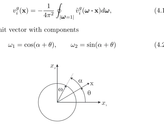
i.e. _f˙_j_δ₍_x₎_{. Introducing a plane wave expansion for the incremental}

displacement vg_i of the Green's state

v_ig(x) =− 1 4π2

I

|ω=1|

˜

v_ig(ω·x)dω, (4.1)

whereω is a unit vector with components

ω1 = cos(α+θ), ω2= sin(α+θ) (4.2)

q a w

x

1

x

2

x

Figure 4.1: Reference system, vectorsω,xand anglesθ andα.

with reference to Figure 4.1, the following representation can be obtained from equation (2.35) in the transformed domain

˜

vg_i(ω·x) = (δ1iω2−δ2iω1)(δ1gω2−δ2gω1)

L(ω) [Ci(η|ω·x|) cos (ηω·x)+

+Si(ηω·x) sin (ηω·x)−iπ

2 cos (ηω·x)],

(4.3)

(44)

4.2. The boundary integral equation

where Ci and Si are the cosine integral and sine integral functions, re-spectively, and

L(ω) =µ(1 +k)ω4₂

ω₁2 ω2 2

−γ1 ω 2 1 ω2 2 −γ2

>0, (4.4)

with

η = Ω

r _ρ

L(ω). (4.5)

The gradient of the incremental displacement (4.1) can be written as

vg_i,k(x) =− 1 4π2

I

|ω|=1

˜

v_i,kg (ω·x)dω (4.6)

where

˜

v_i,kg (ω·x) =ωk

δig−ωiωg

L(ω)

1

ω·x−ηΞ(ηω·x)

(4.7)

and

Ξ(α) = sin(α)Ci(|α|)−cos(α)Si(α)−iπ

2 sin(α). (4.8)

The plane wave expansion of (2.35) has been developed in [6] and [7]. Fi-nally the Green's function for incremental nominal stresses can be derived from the constitutive equations (2.13) as

˙

tg₁₁= (2µ∗−p)v₁g_,₁+ ˙πg_, _t_˙g

12= (µ−p)v

g

1,2+ (µ+µk)v

g

2,1,

˙

tg₂₁= (µ−p)v₂g_,₁+ (µ−µk)v₁g_,₂, t˙g₂₂=−(2µ∗−p)v₁g_,₁+ ˙πg.

(4.9)

4.2 The boundary integral equation

The scattered eld vsc satises the extension of the Betti identity

pro-vided in [7,15]

vsc_g (y) = Z

∂B

˙

tijnivg_j(x,y)−t˙g_ij(x,y)nivj

(45)

where ∂B represents the boundary of the shear band, which is made up of two straight lines of length2l, with external unit normals of opposite sign, so that equation (4.10) can be specialized for a shear band to

vsc_g (y) =− Z l

−l

[[˙tij]]nivjg(ˆx1,y)−t˙gij(ˆx1,y)ni[[vj]]

dxˆ1. (4.11)

Because the incremental traction is continuous across the shear band, equations (3.2)(3.3), the following boundary integral equation is ob-tained

v_gsc(y) = Z l

−l

˙

tg_ij(ˆx1,y)ni[[vj]]dxˆ1, (4.12)

which provides the incremental displacement at every point in the body as function of the jump of the incremental displacement [[vj]]across the

shear band.

The gradient of the incremental displacement can be evaluated from the integral equation (4.12) as

v_g,ksc (y) =− Z l

−l

˙

tg_ij,k(ˆx1,y)ni[[vj]]dxˆ1, (4.13)

so that from the constitutive equations (2.13) the incremental stress can be written as

˙

tsc_lm(y) =−_K_lmkg Z l

−l

˙

tg_ij,k(ˆx1,y)ni[[vj]]dxˆ1+ ˙p(y)δlm, (4.14)

where the incremental in-plane mean stress p˙, for the moment unknown,

can be determined from the following boundary integral equation [8]

˙

p(y) = − Z

∂B

˙

tignip˙g(x−y)dlx+ Z

∂B

nivjKijkgp˙g_,k(x−y)dlx

− Z

∂B

vini

4µµ∗−4µ2_∗+µσ−2µ∗σ−σ

2

v₁1_,₁₁(x−y)

−σ

µ+σ 2

v2₂_,₁₁(x−y) +ρΩ2W(x−y) i

dlx,

(4.15)

(46)

4.2. The boundary integral equation

wherep˙g is the incremental in-plane mean stress of the Green's state

˙

pg = ˙πg−σ

2v

g

1,1, (4.16)

in which

˙

πg = ωg(2µ∗−µ)(1−ω

2

g) + (µ−(δ2g−δ1g)σ₂)ω2g

L(ω)

1

ω·x−ηΞ(ηω·x)

+ωgηΞ(ηω·x) (4.17)

and

˜

W =4 (µ−µ∗)ω₂2−σv˜₂2(ω·x) + log|ω·x|. (4.18)

Introducing for∂B the straight boundary of the shear band,x1ˆ ∈[−l, l],

equation (4.15) becomes

˙

p(y) = − Z

∂B

[[ ˙tig]]nip˙g(x−y)dlx+ Z

∂B

ni[[vj]]Kijkgp˙g_,k(x−y)dlx

− Z

∂B

[[vi]]ni

4µµ∗−4µ2∗+µσ−2µ∗σ−

σ2

2

v₁1_,₁₁(x−y)

−σ

µ+σ 2

v₂2_,₁₁(x−y) +ρΩ2W(x−y) i

dlx,

(4.19) which, considering the continuity of incremental tractions, equations (3.2) (3.3), and the continuity of the normal component of the incremental displacement across the shear band (3.4) reduces to

˙

p(y) = Z l

−l

ni[[vj]]Kijkgp˙g_,k(ˆx1,y)dx1.ˆ (4.20)

In order to determine the incremental displacement jump [[vj]],

un-known in equation (4.12), the pointy is assumed to approach the shear

band boundary. Denoting with s the unit vector tangent to the shear

band, the boundary conditions at the shear band become

(47)

so that equation (4.13) can be rewritten as

ˆ

t(₂₁inc)(y) =nlsmKlmkg Z l

−l

˙

tg_ij,k(ˆx1,y)ni[[vj]]dxˆ1. (4.22)

Equation (4.22) represents the boundary integral formulation for the dy-namics of a shear band interacting with an impinging wave. The kernel of the integral equation (4.22) is hypersingular of order r−2 as r → 0,

being r the distance between eld pointx and source pointy

r =|x−y|=p(x1−y1)2−(x2−y2)2. (4.23)

Note that the integral on right-hand side of equation (4.22) is specied in the nite-part Hadamard sense.

The solution for an inclined shear band in an innite medium can be expressed in the inclined reference system sketched in Fig. 3.1.

The components of the vector of incremental displacementsv in the

reference system x1x2, can be expressed in the local reference system

ˆ

x1xˆ2 as

v=Qvˆ, [Q] =

cosϑ −sinϑ

sinϑ cosϑ

, (4.24)

so that, due to the boundary conditions (3.4),

[[vj]] =Qj1[[ˆv1]] =sj[[ˆv1]], (4.25)

equation (4.22) can be given the nal form

ˆ

−l

˙

tg_ij,k(ˆx1,y)nisj[[ˆv1]]dx1,ˆ (4.26)

showing that the dynamics of a shear band is governed by a linear integral equation in the unknown jump of tangential incremental displacement across the shear band faces, [[ˆv1]]. It is worth noting that the gradient

of the Green incremental stress tensor, constituting the kernel of the boundary integral equation, turns out to be the sum of a static part_t˙g(st)

ij,k

and a dynamic part _t˙g(dyn)

ij,k , whose expressions are given in Appendix B,

(48)

4.3. Discretization and numerical procedure

leading to

ˆ

−l

˙

tg_ij,k(st)(ˆx1,y) + ˙tg_ij,k(dyn)(ˆx1,y)

nisj[[ˆv1]]dxˆ1. (4.27)

4.3 Discretization and numerical procedure

The treatment of the boundary integral equation (4.27) requires the de-velopment of an ad hoc numerical procedure, which needs the implemen-tation of a special strategy to enforce the singular behaviour at the band tips, similar to that developed for cracks in [56,57].

Since both eld and source pointsxandylie on thex1ˆ axis, equation

(4.26) can be rewritten as

ˆ

t(₂₁inc)(ˆy) =nlsmKlmkg Z l

−l

˙

tg_ij,k(ˆx,yˆ)nisj[[ˆv]](ˆx)dx,ˆ (4.28)

where the index `1' has been dropped, so that xˆ, yˆand [[ˆv]] replace

re-spectivelyxˆ1 ,yˆ1 and [[ ˆv1]].

The shear band segment is divided into Q intervals [ˆx(q),xˆ(q+1)] (q=

0, . . . , Q−1; ˆx₍₀₎ =−l,; ˆx₍_Q₎=l)and a linear variation of the incremental

displacement jump[[ˆv]]is assumed within each interval, with the exception

of the two intervals situated at the shear band tips, where a square root variation of the incremental displacement jump[[ˆv]]is adopted:

[[ˆv]](ˆx(q)+ζ∆q) = [[ˆv]](q)(1−ζ) + [[ˆv]](q+1)ζ (q= 1, . . . , Q−2), (4.29)

[[ˆv]](ˆx₍_q₎+ζ∆q) = [[ˆv]](q+1)

p

ζ (q= 0), (4.30)

[[ˆv]](ˆx(q)+ζ∆q) = [[ˆv]](q)

p

(49)

Dq

z

0 1 2 Q

2l

Q - 1

x

^(q) ^x(q+1)

Q -2

Figure 4.2: The shear band line is divided inQ-intervals. Within each interval a linear variation of the incremental displacement jump is assumed, with the exception of the two intervals at the shear band tips.

For a more compact form of the following equations, let us dene

˜

Klmkgij =nlsmKlmkgnisj (4.32)

Whenyˆ= ˆx(p)(p = 1, . . . , Q−1) is assumed to be the source point, the relevant integral equation becomes

ˆ

t(₂₁inc)(ˆx₍_p₎) = ˜Klmkgij∆0

Z 1

0

˙

tg_ij,k(ˆx₍₀₎+ζ∆0,xˆ(p)) [[ˆv]](1)

p

ζ dζ

+ ˜Klmkgij p−2 X q=1 ∆q Z 1 0 ˙

tg_ij,k(ˆx(q)+ζ∆q,xˆ(p))( [[ˆv]](q)(1−ζ) + [[ˆv]](q+1)ζ)dζ

+ ˜Klmkgij p X

q=p−1

∆q

Z 1

0

˙

+ ˜Klmkgij Q−2

X

q=p+1

∆q

Z 1

0

˙

+ ˜Klmkgij∆Q−1

Z 1

0

˙

tg_ij,k(ˆx₍_Q−1)+ζ∆Q−1,xˆ(p)) [[ˆv]](Q−1)

p

1−ζ dζ. (4.33)

(50)

4.3. Discretization and numerical procedure

In equation (4.33), the integrals which are singular forxˆ(q)+ζ∆q →xˆ(p) are relevant to the static kernel_t˙g(st)

12 and can be rearranged as

p X

q=p−1

∆q

Z 1

0

˙

tg_ij,k(st)(ˆx(q)+ζ∆q,xˆ(p))( [[ˆv]](q)(1−ζ) + [[ˆv]](q+1)ζ)dζ

= ∆p−1

Z 1

0

˙

tg_ij,k(st)(ˆx₍_p−1)+ζ∆p−1,xˆ(p))[[ˆv]](p)ζ dζ

+∆p

Z 1

0

˙

t_ij,kg(st)(ˆx₍_p₎+ζ∆p,xˆ(p))[[ˆv]](p)(1−ζ)dζ

+∆p−1

Z 1

0

˙

tg_ij,k(st)(ˆx₍_p−1)+ζ∆p−1,xˆ(p))[[ˆv]](p−1)(1−ζ)dζ

+∆p

Z 1

0

˙

tg_ij,k(st)(ˆx(p)+ζ∆p,xˆ(p))[[ˆv]](p+1)ζ dζ,

(4.34)

so that, by means of a change of variable, the integrals can be evaluated as

p X

q=p−1

∆q

Z 1

0

˙

tg_ij,k(st)(ˆx(q)+ζ∆q,xˆ(p))( [[ˆv]](q)(1−ζ) + [[ˆv]](q+1)ζ)dζ

= Z ∆p

−∆p−1 ˙

tg_ij,k(st)(rer) [[ˆv]](p)dr−

1 ∆p−1

+ 1

∆p

Z ∆p

−∆p−1 ˙

tg_ij,k(st)(rer) [[ˆv]](p)r dr

− 1 ∆p−1

Z 0

−∆p−1 ˙

tg_ij,k(st)(rer) [[ˆv]](p−1)r dr+

1

∆p

Z ∆p

0

˙

tg_ij,k(st)(rer) [[ˆv]](p+1)r dr, (4.35) with er = r/r. The non-null nite parts of the above integrals can be

calculated as

Z ∆p

−∆p−1 ˙

tg_ij,k(st)(rer) [[ˆv]](p)dr=T

g ijk(θ)

− 1

∆p−1

− 1

∆p

[[ˆv]]₍_p₎,

− 1 ∆p−1

Z 0

−∆p−1 ˙

tg_ij,k(st)(rer) [[ˆv]](p−1)r dr=Tijkg (θ)

log ∆p−1

∆p−1

[[ˆv]](p−1),

1

∆p

Z ∆p

0

˙

tg_ij,k(st)(rer) [[ˆv]](p+1)r dr=Tijkg (θ)

log ∆p

∆p

[[ˆv]](p+1)

(51)

In the particular cases when yˆ = ˆx(p) is assumed to be the source point andp= 1 or p=Q−1, equation (??) has to be rewritten as

ˆ

t(₂₁inc)(ˆx(p)) = ˜Klmkgij∆0

Z 1

0

˙

tg_ij,k(ˆx(0)+ζ∆0,xˆ(p)) [[ˆv]](1)

p

ζ dζ

+ ˜Klmkgij∆1

Z 1

0

˙

tg_ij,k(ˆx(1)+ζ∆1,xˆ(p))( [[ˆv]](1)(1−ζ) + [[ˆv]](2)ζ)dζ

+ ˜Klmkgij Q−3 X q=2 ∆q Z 1 0 ˙

+ ˜Klmkgij∆Q−2

Z 1

0

˙

tg_ij,k(ˆx₍_Q−2)+ζ∆Q−2,xˆ(p))( [[ˆv]](Q−2)(1−ζ)+[[ˆv]](Q−1)ζ)dζ

+ ˜Klmkgij∆Q−1

Z 1

0

˙

tg_ij,k(ˆx₍_Q−1)+ζ∆Q−1,xˆ(p)) [[ˆv]](Q−1)

p

1−ζ dζ. (4.37)

When p= 1, the nite parts of singular integrals can be evaluated as

∆0

Z 1

0

˙

tg_ij,k(st)(ˆx(0)+ζ∆0,xˆ(p)) [[ˆv]](1)

p

ζ dζ

+ ∆1

Z 1

0

˙

t_ij,kg(st)(ˆx(1)+ζ∆1,xˆ(p)) [[ˆv]](1)(1−ζ)dζ

=T_ijkg (θ)

− 9

8∆0

−ln ∆0

2∆0

− 1

∆1

−ln ∆1

∆1

[[ˆv]](1), (4.38)

while, when p =Q−1, the nite parts of the singular integrals can be

evaluated as

∆Q−2

Z 1

0

˙

tg_ij,k(st)(ˆx(Q−2)+ζ∆Q−2,xˆ(p)) [[ˆv]](Q−1)ζ dζ

+ ∆Q−1

Z 1

0

˙

tg_ij,k(st)(ˆx(Q−1)+ζ∆Q−1,xˆ(p)) [[ˆv]](Q−1)

p

1−ζ dζ

=T_ijkg (θ)

− 9

8∆Q−1

−ln ∆Q−1

2∆Q−1

− 1

∆Q−2

−ln ∆Q−2

∆Q−2

[[ˆv]](Q−1). (4.39)

(52)

4.4. Validation of the numerical procedure

Hence, using a collocation method, thus assuming p = 1, . . . , Q−1, a

system ofQ−1 algebraic equations is obtained which can be written in

matrix form as follows

n ˆ

t(₂₁inc)

o

= [C]{[[ˆv]]}, (4.40)

withCthe matrix of the coecients.

The nominal shear traction_tˆ(inc)

21 generated by a shear wave impinging the shear band can be obtained using equations (2.34) and (2.13) into equation (3.12), thus yielding

ˆ˙

t(₂₁inc)(x) =τ0ei

Ω

c(p·x−ct)(n2

1(η−1)−(1−k)n22) cos2θ0

+ (n2₂(η−1) + (1 +k)n2₁) sin2θ0

+n1n2(η−2ξ) sin 2θ0

.

(4.41)

whereτ0=iAµΩ/cis the maximum shear stress acting at the shear wave front in the quasi-static limit,Ω→0. For a wave traveling orthogonally

to the shear band, equation (4.41) reduces to a positive quantity, at least until strong ellipticity holds true.

4.4 Validation of the numerical procedure

A shear band is discretized withQ= 100 line elements and numerically

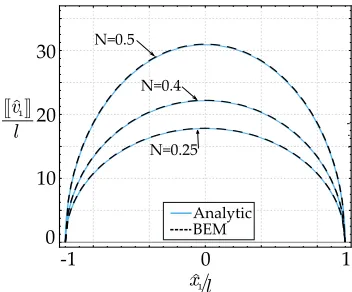
analyzed when inside a ductile metal whose behaviour is described by the J2-deformation theory of plasticity. A validation of the developed numerical technique can be obtained, in the limit Ω → 0, by

compar-ing with the analytic solution for the static case provided by Bigoni and Dal Corso [9]. This validation is provided in Figure 4.3, where the mod-ulus of the displacement jump [[ˆv1]] (divided by the semi-length of the

shear band) is plotted along the shear band line x1ˆ . The validation

turns out to be excellent, as the analytic solution is superimposed to the numerical solutions, for dierent values of the hardening exponent N (0.25,0.4,0.5), at respective levels of prestrain close to the elliptic

(53)

The convergence of the numerical solution to the static -analytical-solution (developed in [9]) is shown in Figure 4.4, where the (percent) error in the incremental displacement jump [[ˆv]]q, evaluated at the middle

of the shear band, xˆ1/l = 0, is reported as a function of the number of the collocation points Q.

1

^ x/_l

0 1

-1

v

l

1

^

10 20 30

0

Anal ticy

BEM N=0.4 N=0.5

N=0.25 [[ [ [

Figure 4.3: The quasi-static behaviour of a shear band loaded with a remote shear (obtained numerically in the limitΩ→0) is compared with an available analytical solution for dierent hardening exponentsN and prestrains near the elliptic border. Modulus of dimensionless displacement jump along the shear band line,xˆ1/l, for theJ2-deformation theory of plasticity and three hardening exponents N(0.25,0.4,0.5).

Two dierent sets of shape functions are considered, namely, linear shape functions for the whole shear band in one case (circular spots), while in the other case square-root shape functions are used only in the element at the shear band tip (square spots). It can be seen that in the middle of the shear band for Q = 100 the error is about 1% for both

shape function sets.

(54)

4.4. Validation of the numerical procedure

v(

q

)

^_[[

[[

Error % of

Number of discretization Q 0

0 100 200 300 400 500

4 8 10

2 6

N=0.4

Figure 4.4: Percent error in the incremental displacement jump[[ˆv]]q for dier-ent numbers of collocation pointsQ(10,20,50,100,200,500), and for two sets of shape functions (N = 0.4 has been considered). The errors are evaluated at the middle of the shear band,xˆ1/l= 0, note that the circular and square spots are practically superimposed forQ>200.

With Q = 100 elements and the selected shape functions, the

(55)

(56)

5 Results for an isolated shear

band

In this Chapter results pertaining to an isolated shear band are reported for two dierent constitutive equations: for a J2-deformation theory of plasticity with hardening exponent N = 0.4, and for a Mooney-Rivlin

material.

5.1 Results for the

J

2

-deformation theory of

plas-ticity

A shear band is discretized withQ= 100 line elements and numerically

analyzed when inside a ductile metal whose behaviour is described by the J2-deformation theory of plasticity. The incremental moduli are provided by equations (2.54) and the hardening exponent is assumed to beN = 0.4,

so that ellipticity is lost at the critical value of the logarithmic strain ε1 ≈0.678. Results are presented below.

5.1.1 Wave propagation normal to the shear band

(57)

Chapter 5. Results for an isolated shear band

loaded. The numerical solution of the linear system (4.40) allows to com-pute the longitudinal displacement jump across the shear band, [[ˆv1]].

The dynamic shape of the displacement jump along the shear band line is reported in Figure 5.1, referred to a prestrain ε1 = 0.667, close to the boundary of ellipticity loss. This gure shows that, near the reso-nance frequency, the displacement jump along the shear band assumes the quasi-static shape, but at high frequency displays a markedly dif-ferent behaviour [37], namely, it decades in amplitude and displays an oscillation (see the pink curve referred to Ωl/c1 = 6).

x l / 1 ^ 0 -1 v

v(st) 1 ^ 1 ^

|

0 0.4 0.8 1.2 [[ [[ [[ [[ 6 = l W_c 1 3 = l W c1 2 = l W c1 0 = l W c1 1 = l W c1 1

Figure 5.1: Modulus of dimensionless displacement jump along the shear band line,xˆ1/l, for theJ2-deformation theory of plasticity: dierent wavenumber are considered withN = 0.4and prestrainε1= 0.667.

The variation with the wavenumber, Ωl/c1, (of the modulus) of the displacement jump[[ˆv1]](normalized with respect to the quasi-static value [[ˆv(₁st)]]) is shown in Figure 5.2 for several values of prestrain, ranging from

0 to ε1 = 0.667. In this gure the maxima of the curves represent reso-nance condition (the displacement grows, but does not blow-up to innity, due to the radiation damping, properly accounted for in the numerical solution), so that it is clear that an increase in the prestrain leads to an amplication factor which grows from 20%, occurring at null prestrain,

to 41%, occurring at a prestrain close to the border of ellipticity loss.

(58)

5.1. Results for theJ2-deformation theory of plasticity

Results not reported for brevity show that a decrease in the hardening exponentN shifts the resonance towards higher frequencies.

3 4 6

2 1 5 0 0 0.2 0.4 0.6 0.8 1.0 1.2 1.4 v1

^

|

( = )x^₁ 0

|

v1

^( = )x^₁ 0

[[ [[

[[ (st) [[

l W c1 =0.01 e1 =0.05 e1 =0.10 e1 =0.15 e1 =0.21 e1 =0.27 e1 =0.34 e1 =0.43 e1 =0.55 e1 =0.67 e1

Figure 5.2: Modulus of dimensionless displacement jump in the middle of the shear band (xˆ1= 0) is plotted as a function of the dimensionless frequency for dierent values of prestrain and for theJ2-deformation theory of plasticity with N = 0.4 and limit prestrain ε1 = 0.667 at the EC/H boundary. Note that a resonance frequency is visible (the peak of the curves) and that this resonance becomes more evident at increasing prestrain, when it approaches the elliptic boundary.

The stress concentration at the shear band tips can be investigated using the Stress Intensity Factor (SIF) and because only incremental shear stresses are acting on the band, a Mode II SIF is adopted, which is dened as

KII = lim

ˆ

x1→l+ ˆ˙

t21(ˆx1,x2ˆ = 0)p2π(ˆx1−l) (5.1)

which in the quasi-static case becomes

Kst = ˆ˙t∞

√

(59)

The SIF is also dened as a function of the displacement jump in the form [3,18]

KII =

µ√2π

4(1−ν)

[[ˆv]](1)

√

∆0

, (5.3)

where [[ˆv]]₍₁₎ is the displacement jump evaluated at the rst inner node

from the tip of the shear band. Figure 5.3 reports the SIF, KII,

nor-malized through the quasi-static condition K_II(st), as a function of the wavenumber. ● ● ◆ ◆ ◆ ◆ ◆ ◆ ◆ ◆ ◆ ◆

l

W

c

1

0 1.0 1.5

0.2 0.4 0.6 0.8 1.0 1.2 1.4 KII KII

(st)

0.0 ◆ ◆ ◆ ◆ ◆ ◆ ◆ ◆ ◆ ◆ ◆ ◆ _{◆ ◆ ◆} ◆ ◆ ◆ _◆ ◆ ◆ =0 b

= /6p b

= /2p b Chen & Sih

=0 b

= /6p b

= /2p b BEM

◆ ◆

◆

Figure 5.3: Modulus of dimensionless mode II Stress Intensity Factor at the shear band tip as a function of the wavenumber; a comparison with the analyt-ical solution of Chen and Sih [17], with null prestrain in the isotropic case with

µ=µ∗.

It has to be noted that Chen and Sih [17] developed an analytical solution for the SIF pertinent to a crack impinged by an incident shear wave in a linear elastic and isotropic body. This solution can be used to validate the developed numerical procedure, as reported in Figure 5.3, relative to a null prestrain. Here the absolute value of the SIF (normalized

(60)

with respect to the quasi-static limit) is reported as a function of the wavenumber. The validation turns out to be satisfactory because, for the tested anglesβ of the wave propagation, the discrepancy is within 8%.

3 4 6

2

1 5

0

l

W

c

1

=0.01

e1 =0.21

e1 =0.43

e1 =0.55

e1 =0.67

e1

5 10 15

0

KII KII

(st)

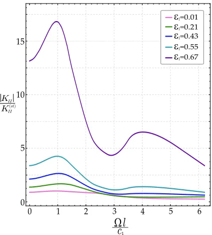
Figure 5.4: Modulus of dimensionless mode II Stress Intensity Factor at the shear band tip as a function of the wavenumber for dierent levels of prestrain for aJ2-deformation theory withN = 0.4.

The dimensionless SIF for the shear band tips at dierent levels of prestrain is reported in Figure 5.4 as a function of the dimensionless fre-quency. In the quasi-static limit and for a null prestrain the SIF correctly tends to 1, while, when the elliptic boundary is approached, the SIF blows up, reaching a value approximately 15 times the quasi-static value for a prestrain ε1 = 0.66, whereas at the elliptic border it grows to innity, coherently with the quasi-static behaviour, [9]. This is once more the evidence of a resonance condition, with an increase of 41% of the SIF

(61)

band produces a resonance, evidenced through a substantial growth in the jump of displacement across the shear band and in the stress intensity factor at the shear band tip.

5.1.2 Wave propagation inclined or parallel to the shear band

A wave obliquely impinging a shear band is now considered, with p·n

dierent from both 0 and 1. The shear traction can be derived from equation (4.41) and is composed of a real symmetric part and an imagi-nary skew-symmetric part. Therefore, the traction is non-symmetric with respect to the xˆ2-axis.

This can be noted in Figure 5.5, where, as in Figure 5.1, the dimen-sionless displacement jump is reported along the shear band line as a function of the dimensionless frequency, for various inclinations of the wave propagation vector. When the wave propagation is inclined at an angle β belonging to the interval (−π/2 +θ0, π/2 +θ0), the maximum

value of the displacement jump shifts towards the right tip of the band. Due to the fact that the wave is now inclined with respect to the shear band, the stress intensity factors at the tips of the shear band are dierent [62], see Figure 5.6, where the dimensionless SIF for the two tips (one denoted by `+' and the other by `−') are reported as functions

of the dimensionless frequency. It can be observed that the higher the displacement jump, the higher is the SIF, moreover a wave orthogonal to the shear band produces the largest value of the SIF and therefore the maximum resonance.

(62)

0 =

l

W_c

1 =1

l W_c 1 = l W_c

1 p₂ =

l W_c 1 = l W_c 1 = l W_c

1 2p

p

3 2

v v(st)

1 ^ 1 ^

|

[[ [[ [[ [[ v v(st)

1 ^ 1 ^

|

[[ [[ [[ [[ x1 x2 q0 b p v v(st)

1 ^ 1 ^

|

[[ [[ [[ [[

(63)

3 4 6

2 1 5 0 5 10 15 0 5 10 15 0 0 20 20

3 4 6

2 1 5 -KII KII (st)

l W c1 l W c1 KII KII (st)

+ -x1 x2 q0 =p/2 b + -x1 x2

=q +p/2

q0 0 b + -x1 x2 q0

=q0

b + -x1 x2 q0 =0 b

Figure 5.6: SIF at the left `−' and right `+' tips of a shear band (in a J2 -deformation theory of plasticity material with N = 0.4), for dierent inclina-tionsβ of the wave propagation (0, θ0, π/2, π/2 +θ0).

(64)

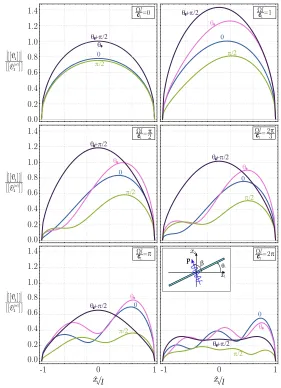
5.1.3 Incremental strain elds

The modulus of the incremental strain eld (which is deviatoric, because of incompressibility) dened as (vi,jvi,j+vi,jvj,i)/2, can be computed

by using the gradient of the incremental displacement, equation (4.13), in the constitutive equations (2.13). In the following the modulus of the incremental strain eld is computed by using the real part of the gradient of incremental displacement, so that the phase shift related to the imaginary part is not considered. The modulus of the incremental strain eld, computed at a prestrain level of ε1 = 0.667 (i.e. close to

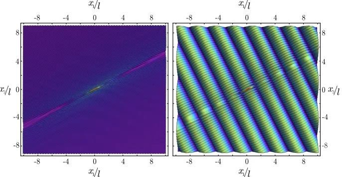
the elliptic boundary) is reported in Figure 5.7, in terms of scattered wave eld (on the left) and in terms of total wave eld (on the right). Two incident waves with wavenumber Ωl/c1 = 1 are considered, one

orthogonal to the shear band (with inclination β = θ0 +π/2) and the

other aligned parallel to the x1−axis (with inclination β = 0). These inclinations of propagation represent the directions along which the wave velocity c assumes the minimum and maximum values respectively, see equation (3.16).

It is worth noting that the wavenumber Ωl/c1 = 1used for the

com-putations corresponds to a wavelength in the direction orthogonal to the shear band,2πlc/c1, which is approximately 1/6 of the shear band length, thus much greater than the shear band thickness.

It can be noted that for both wave inclinations, the scattered eld turns out to be a family of plane waves parallel to the shear band. The eect of this scattered eld on the total strain eld is to produce a ne texture of parallel vibrations, which superimposes on the impinging wave eld. The texture shows a narrow conical shadow zone emanating from the shear band tips, where the scattered eld is strongly attenuated and tends to disappear. This eect becomes more visible in the case ofβ = 0,

because incident and scattered waves propagate in dierent directions, rather than in the case of wave travels orthogonal to the band. In the case of an incident wave with wavenumber Ωl/c1 = 1,

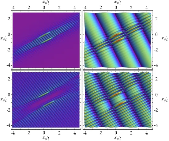
propagat-ing in the direction parallel to the shear band, Figure 5.8 represents the scattered and total strain elds for three increasing levels of prestrain (ε1 = 0.43, ε1 = 0.55, ε1 = 0.66). Starting from the lowest level of

(65)

0 4 8

-4

-8 -8 -4 0 4 8

4

-4

0 8

-8

4

-4 0 8

-8

4

-4

0 8

-8

4

-4 0 8

-8

0 4 8

-4

-8 -8 -4 0 4 8

=0

b =q +p/2

b 0

x l2/

Figure 5.7: Scattered (left) and total (right) incremental strain eld produced by a wave incident to a shear band (in a J2-deformation theory of plasticity material withN = 0.4) orthogonally to it (β=θ0+π/2) or aligned parallel to thex1−axis (β = 0). The wavenumber is Ωl/c1 = 1and the level of prestrain isε1= 0.667, close to the elliptic boundary.

to become narrower when the elliptic boundary is approached.

(66)

4

-4 0 8

-8 =0.43

4

-4 0 8

-8

0 -4 -8

=0.67

4

-4 0 8

-8 =0.55

e1

x l1/ x l1/

x l2/

4 8 -8 -4 0 4 8

0 -4

-8 4 8 -8 -4 0 4 8

4

-4 0 8

-8

4

-4 0 8

-8 4

-4 0 8

-8

(67)

The shadow zone is analyzed near the elliptic boundary as a func-tion of the frequency, in particular, the upper left quarter of the map of the incremental strain eld is reported in Figure 5.9 for two frequencies (Ωl/c1 = π/5,Ωl/c1 = π/2). This plot reveals that the shadow zone becomes more visible at frequencies higher than the value corresponding to resonance.

0 2 4 6 0 2 4 6

0 2 4 6 0 2 4 6 0

x l1/ x l1/

x l2/

=p/5

l W

c1

= p/2

l W

c1

2 4 6 8 10 0 2 4 6 8 10

0 2 4 6 8 10 0 2 4 6 8 10

Figure 5.9: Incremental strain eld near a shear band (in a J2-deformation theory of plasticity material with N = 0.4) produced by a wave impinging parallel to the shear band,β=θ0and waveleghtΩl/c1=π/5(upper part) and Ωl/c1=π/2(lower part).

(68)

5.2. Results for a Mooney-Rivlin material

5.2 Results for a Mooney-Rivlin material

A shear band in a Mooney-Rivlin material, emerges and grows parallel to theσ1-principal axis, with a null inclination,θ0 = 0. In order to approach the elliptic/parabolic boundary, the limit of the prestressk →1 (which

formally correspon