96
Copyright © 2018. IJEMR. All Rights Reserved.
Volume-8, Issue-2, April 2018
International Journal of Engineering and Management Research
Page Number: 96-102
Vector Autoregressive (VAR) for Rainfall Prediction
Tita Rosita1, Zaekhan2 and Rachmawati Dwi Estuningsih3
1,3Lecturer, Department of Statistics, Polytechnic of AKA Bogor, INDONESIA 2Assistant Professor, Graduate Program in Economics, Universitas Indonesia, INDONESIA
1Corresponding Author: [email protected]
ABSTRACT
Weather and climate information is useful in a variety of areas including agriculture, tourism, transportation both land, sea and air. For that, up to date weather and climate data and its forecasting are essential. This study aims to create rainfall modeling with Vector Auto Regressive (VAR) using circular data and linear data. The data used comes from the station climatology Darmaga Bogor period 2006-2017. The VAR model (2) of the rainfall variables in the t-month is affected by the t-1 moisture air moisture, the t-2 moisture air and the air temperature at t -2. This VAR model (2) is used to forecast the next period. The mean absolute percentage error (MAPE) VAR (2) obtained was 42.18. The novelty of the study is (1) VAR modeling for rainfall prediction, (2) Use of circular data for wind direction data.
Keywords-- Vector Auto Regressive (VAR); Circular Data; Rainfall
Type of Paper:Empirical. MSC Classification: 62P99 JEL Classification: C32, C51, C53.
I.
INTRODUCTION
Weather is a state of air at any given moment and in a relatively narrow area and in a short period of time in hours or days (Tjasjono, 2004). Climate is the average weather condition within a year that the investigation is done for a long time (minimum 30 years) and covers a large area (Tjasjono, 2004). Weather and climate have elements such as light, air humidity, air temperature, air pressure, wind (wind direction and speed) and rainfall. Information on weather and climate is useful in a variety of areas including agriculture, tourism, transportation both land, sea and air.
Up-to-date climate data and its forecast for several future periods are important. Forecasting method for rainfall time series data, air humidity, air temperature, air pressure, wind direction and wind speed can be done by single time series model forecasting technique and can be simultaneously done. This is
because the movement of time series data can occur together or follow the movement of other time series data. One of the most commonly used forecasting methods is Vector Autoregressive (VAR). VAR is widely used mainly in the field of econometrics. In VAR the system of equations shows that each variable as a linear function of the constant and the past value (lag) of the variable itself and the lag value of the other variables present in the system (Enders, 1995).
The dynamic relationship between the movement of interrelated variables and the reciprocal effect of the weather is an interesting topic to examine. The choice of six variables namely rainfall, air humidity, air temperature, air pressure, wind direction and speed in this study because it is assumed there is a reciprocal relationship and relationship between six variables. In addition, Tjasjono (2004) also states that rain is a symptom or a weather phenomenon that is seen as a non-free variable formed from various elements of the weather.
Based on the explanation above, in this research will be formed a VAR model using six variables, namely rainfall, air humidity, air temperature, air pressure, wind direction and wind speed. The wind direction is a circular variable, ie a variable measured in units of degrees that can be represented in a circle of radius of one unit. The position of each data in the circle depends on the selection of the zero point and the direction of rotation. Therefore, in the data analysis the variable of wind direction is divided into component sin direction and cos direction.
II.
RESEARCH OBJECTIVES
97
Copyright © 2018. IJEMR. All Rights Reserved.
III.
DATA AND METHODOLOGY
Data
The data used in this research is secondary data of monthly weather element that is rainfall, air humidity, air temperature, air pressure, direction and wind speed of Darmaga Bogor region from January 2006 to December 2017. In this research, the data is divided into two, namely January data 2006- December 2015 used for VAR modeling and data from January 2016- December 2017 as validation data.
Methodology
Stages of Data Analysis:
Conducting exploration of data on each variable. Exploration of data conducted among them determine the descriptive statistics that is the measure of central symptoms (average), the size of the spread (minimum value, maximum value, and standard deviation).
Conduct a test of data kestasioneran for each variable. The kestasioneran of each variable can be checked through the Dickey Fuller test (Enders, 1995). The test kestasioneran data following the order autoregresi process 1. Suppose the time series data yt single variable is
written:
with a distinction model can be written as:
The hypothesis to be tested is:
H0 : (data is not stationary)
H1 : (data is stationary)
The value is assumed by the least squares method by making the regression between and as well as
the tests performed using t-test. Test statistics can be written as follows:
̂
̂
where ̂ indicates the value of conjecture and ̂
indicates the standard deviation from ̂. Decision:
If the tstat value < is critical value in the Dickey Fuller
table, then reject Ho which means the data is stationary.
Selects the lag of the VAR model
If the VAR order is denoted by p, then each n equation contains n × p coefficient coupled with an intercept. According to Enders (1995), the VAR order can be determined by using AIC (Akaike Information Criterion). The AIC measures the goodness of the model that improves the loss of degrees of freedom when additional lag is included in the model. The order of VAR is determined by the value of p which produces the smallest AIC.
According to Enders (1995), the test criteria for determining the order of VAR with AIC statistics are:
| |
where | | indicates the determinant of the covariance variance matrix error, indicates number of observations, N indicates the expected number of parameters of all equations. If each equation in n
variables VAR has plag and intercept, then N = n2p + n
(Enders, 1995).
Make predictions of model parameters
Vector Autoregressive (VAR) is a system of equations involving each variable as a linear function of the constants and lag (past) of the variable itself and the lag value of other variables present in the system (Enders 1995). How to estimate the VAR model with the least squares method (Ordinary Least Square, OLS) in each equation separately.
In general the model VAR of order p for n
variables can be formulated as follows (Enders, 1995):
where indicates n × 1 sized vector containing n
variables included in the VAR model at time t and t-i, i = 1,2, ... p, indicates intercept vector of n × 1 size,
n × n coefficient matrix for each i = 1,2, ... p,
indicates the n × 1 sized vector sizes are 1, 2, ....,
𝑛 , p indicates order VAR, t indicates observation period.
Assesses the impulse response and decomposition response functions
IRF informs the effect of shock change or shock of a variable on the forecast of the variable itself and other variables (Enders, 1995). Decomposition of variance decomposes the change of values of a variable caused by the shock of the variable itself and the shock of other variables.
Suppose the order VAR model 1 with the equation:
and the number of endogenous variables 2 (x_t and z_t), then the forecast for the next step is (Enders, 1995):
E(yt+m) = (I+A1+ A12+ ... + A1m-1) A0 + A1myt
with forecast error of:
yt+m - E(yt+m) = =
where [
]
The coefficient can be used to generate the effect of the shock of the variable or ( or ) to the series or . For example, the coefficient is
the direct influence of a unit of change to . In the same way, elements and are the response of unit changes and at . In the nth period, the
effect of on the value of is 𝑛 . The coefficients , , and are
referred to as impulse response functions. The effect of the shock can be seen visually by ploting the coefficients
with i.
Forecasting / validating models
98
Copyright © 2018. IJEMR. All Rights Reserved.
MAPE = | ̂|
where indicates actual data and ̂ indicates forecast data. The smaller the MAPE value, the data forecasting results closer to the actual value.
In summary the above steps are presented in Figure 1.
Figure 1 Stages of modeling
IV.
RESULTS AND DISCUSSION
Data Exploration
Results Exploration of data on all variables are as follows:
Table 2. Descriptive Statistics of Linear Variables
Variables Rainfall (mm) Humidity (%) Air Temperature
(0C) Air pressure (mb)
Wind velocity (knot) Mean 303,9378 82,8141 25,8448 1012,1160 6,4248 Max 855,0000 90,0000 27,1000 1017,1000 14,0000
Min 2,0000 70,0000 24,4400 1009,1000 3,1000
Deviation Standar 168,9247 4,4259 0,4628 1,4755 2,0451
Descriptive statistics of wind direction variables are separate from other variables. This is due to the wind direction variable is the circular data, so to determine the
descriptive statistics and the graph is different from the variables with the linear scale. The descriptive statistics of wind direction variables are presented in Table 3.
Table 3 Descriptive statistics of wind direction variables Variables Wind direction
Mean Directions ̅ 300,417°
Mean Length of Response Vector | ̅| 0,702
Concentration ( ̂) 2,019
Circular Variance 0,298
is 271.219 °. This shows during 2001-2008 the direction of wind tends to come from the northwest. The average resultant vector length | ̅|
99
Copyright © 2018. IJEMR. All Rights Reserved.
2006-2015 the wind direction varies or does not converge to a particular value (Fisher, 2000). The value of circular variance of 0.298 gives the meaning that the circular data (wind direction) is quite varied. For wind direction data for the last eight years, cos component direction and sin direction correlate closely (r = 1) or in other words multicollinearity occurs. So in making the VAR model, the wind direction component used is chosen one. In this study the wind direction component used is cos direction.
Stationary Data
There is an assumption that must be met in VAR analysis that is checking kestasioneran data. The kestasioneran data checking is done by Dickey Fuller test. The data analysis is conducted to test whether the variables of rainfall, humidity, air temperature, air pressure, wind speed and cos wind direction are stationary or not. The results of the test kestasioneran data presented in Table 4.
Table 4. Dickey Fuller test for the stationary data
Variables I(0)
t-stat Critical value Explanation
Rainfall -8,2048 -2,8859 Stationary
Air Humidity -6,6108 -2,8867 Stationary
Air Temperature -6,3041 -2,8859 Stationary
Air pressure -3,6154 -2,8859 Stationary
Wind velocity -3,7082 -3,4483 Stationary
Cos direction -3,2150 -2,8861 Stationary
Based on Table 4, all variables are stationary at α = 0 05 so there is no need for differencing. The model used is a standard VAR model. Determination of Order of VAR
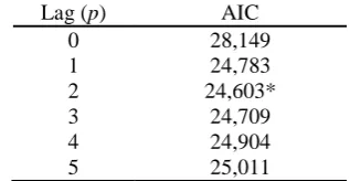
The determination of the order or length of the VAR model lag is done by examining the AIC (Akaike Information Criteria) value. The AIC value calculation results are presented in Table 5.
Table 5. AIC calculation results for selection of VAR order Lag (p) AIC
0 28,149
1 24,783
2 24,603*
3 24,709
4 24,904
5 25,011
* Indicates selected order or song based on AIC criteria
Based on Table 5, when p = 1 obtained the smallest AIC value so that the order of VAR model is order 2 or written VAR (2). The VAR model (2) can be written as follows:
where indicates vector size 6×1 containing 6 variables included in the VAR model in month t, indicates
vector size 6×1 containing 6 variables included in the
VAR model in month t-1, indicates intercept vector
6×1, indicates coefficient matrix measuring 6×6,
indicates the remaining vector is 6×1 in month t. Estimation of Order VAR Model 2
The VAR model estimation is done by the least squares method. The VAR model used in this research is the order VAR 2. The result of the assumption of the parameter of the order VAR model 2 is as follows:
Raint = 17865,79 + 0,0859 Raint-1 – 0,1032 Raint-2 + 19,1994 Humidt-1* – 19,6022 Humidt-2* + 73,3649 Tempt-1 99,0169
Tempt-2* – 15,1756 Presst-1 – 1,5177 Presst-2 + 14,5238 Veloct-1 – 8,7751 Veloct-2 – 19,3487 Cost-1 + 0,9104 Cost-2.
Humidt = 453,958 + 0,0031 Raint-1 + 0,0004 Raint-2 + 0,6939 Humidt-1* – 0,1345 Humidt-2 + 2,0189 Tempt-1* – 0,8754
Tempt-2 – 0,6154 Presst-1 + 0,1722 Presst-2 + 0,0203 Veloct-1 + 0,1244 Veloct-2 – 1,6043 Cost-1* + 0,2705 Cost-2.
Tempt = –48,6209 + 0,0001 Raint-1 + 0,0000 Raint-2 – 0,0141 Humidt-1 – 0,0056 Humidt-2 + 0,4365 Tempt-1* – 0,1688 Tempt
-2 + 0,0384 Presst-1 + 0,0297 Presst-2 + 0,0392 Veloct-1 – 0,0127 Veloct-2 + 0,2229 Cost-1* – 0,1758 Cost-2.
Presst = 157,7907 – 0,0002 Raint-1 – 0,0003 Raint-2 – 0,0932 Humidt-1* + 0,1078 Humidt-2* – 0,5939 Tempt-1* + 0,7657
Tempt-2* + 0,6115 Presst-1* + 0,2269 Presst-2* + 0,0319 Veloct-1 + 0,0398 Veloct-2 – 0,3887 Cost-1* – 0,1102 Cost-2.
Veloct = –37,8283 – 0,0001 Raint-1 + 0,0004 Raint-2 + 0,0062 Humidt-1 – 0,0590 Humidt-2 + 0,0285 Tempt-1 – 0,5986 Tempt
-2* – 0,0770 Presst-1 + 0,1338 Presst-2 + 0,4769 Veloct-1* + 0,4411 Veloct-2* + 0,6394 Cost-1* – 0,0179 Cost-2.
Cost = –2,3248 – 0,0000 Raint-1 – 0,0003 Raint-2 + 0,0029 Humidt-1 +0,0250 Humidt-2 + 0,0411 Tempt-1 + 0,0843 Tempt-2 +
0,0939 Presst-1 – 0,0578 Presst-2 + 0,0627 Veloct-1 - 0,0578 Veloct-2 + 0,4139 Cost-1* + 0,2985 Cost-2*.
100
Copyright © 2018. IJEMR. All Rights Reserved.
Based on the VAR model for rainfall above, it is found that the variables that have significant influence on rainfall in month t are the air humidity variables in month t-1, the humidity of air in month t-2 and the air temperature in month t-2. Tjasjono (2004) says that rainfall is seen as one of the most important forecasts of weather and climate variables. This is because rainfall affects human life activities in various sectors such as agriculture, transportation, trade, health, environment
and so on and has a very high diversity both by time and place. Therefore, for the next variables that will be discussed more deeply is the variable of rainfall.
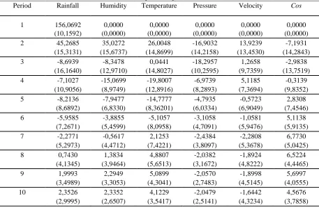
Impulse Response Function
The Impulse Response Function (IRF) function informs the effect of the shock of a variable on the forecast of the variable itself and other variables (Enders 1995). The IRF results from the rainfall variables are presented in Table 6 below:
Table 6. Function of Impulse Response variables Rainfall
Period Rainfall Humidity Temperature Pressure Velocity Cos
1 156,0692 0,0000 0,0000 0,0000 0,0000 0,0000 (10,1592) (0,0000) (0,0000) (0,0000) (0,0000) (0,0000) 2 45,2685 35,0272 26,0048 -16,9032 13,9239 -7,1931 (15,3131) (15,6737) (14,8699) (14,2158) (13,4530) (14,2843) 3 -8,6939 -8,3478 0,0441 -18,2957 1,2658 -2,9838
(16,1640) (12,9710) (14,8027) (10,2595) (9,7359) (13,7519) 4 -7,1027 -15,0699 -19,8007 -6,9739 5,1185 -0,3139
(10,9056) (8,9749) (12,8916) (8,2893) (7,3694) (9,8352) 5 -8,2136 -7,9477 -14,7777 -4,7935 -0,5723 2,8308
(8,6892) (6,8330) (8,36201) (6,0334) (6,9049) (7,4546) 6 -5,9585 -3,8855 -5,1057 -3,1058 -1,0581 5,1138
(7,2671) (5,4599) (8,0958) (4,7091) (5,9476) (5,9135) 7 -2,2771 -0,5617 2,1253 -2,4384 -2,2808 6,7730
(5,2973) (4,4712) (7,4221) (3,8097) (5,3678) (5,0425) 8 0,7430 1,3834 4,8807 -2,0382 -1,8924 6,5224
(4,1345) (3,9464) (5,6513) (3,1672) (4,8222) (4,4465) 9 1,9993 2,2949 5,0899 -2,0570 -1,8998 5,6997
(3,4989) (3,3053) (4,3041) (2,7483) (4,5145) (4,0555) 10 2,3526 2,3352 4,1229 -2,0479 -1,6442 4,5676
(2,9995) (2,6507) (3,5417) (2,5141) (4,3234) (3,7858)
The table above shows how the six variables in the VAR system respond when a standard 1 deviation shock occurs in rainfall. Shock of 1 standard deviation on rainfall in month t resulted in a standard deviation error 156,0692 of the unit against forecasting rainfall one month ahead, but did not give effect to the standard deviation error other weather elements in forecasting one month ahead (standard deviation error other variables zero). For forecasting for the next two months, the standard deviation of the rainfall error will be 45.2685 above the average. While the effect on other variables is to give rise of standard deviation of air humidity error error of 35,0272 above average, the increase of standard deviation of error of temperature variable is 26,0048 above average, decrease of standard deviation error of air pressure variable of 16, 9032 above the average, the
standard deviation of the wind speed variation error by 13.9239 above the mean and the standard deviation of the wind direction deviation error of 7.1931 below the mean.
In general, the shock on the rainfall of all variables gives an influence big enough until the sixth month. After that period the effect of rainfall shock on other variables tends to be constant and convergent to zero after a period of six months.
Variance Decomposition
Variance Decomposition (VD) informs the proportion of diversity forecasting errors of a variable described by the error of each variable and other error variables (Enders, 1995). Here is the result of the decomposition of variations of the rainfall variables.
Table 7. Decomposition of Various Rainfall Variables
Period S.E. Rainfall Humidity Temperature Pressure Velocity Cos A
101
Copyright © 2018. IJEMR. All Rights Reserved.
3 171,2654 90,2855 4,4205 2,3055 2,1153 0,6664 0,2068 4 173,4255 88,2182 5,0662 3,5520 2,2246 0,7371 0,2019 5 174,5186 87,3381 5,2103 4,2247 2,2723 0,7289 0,2257 6 174,8437 87,1297 5,2403 4,2943 2,2954 0,7299 0,3105 7 175,0353 86,9559 5,2299 4,2996 2,3098 0,7453 0,4595 8 175,2539 86,7409 5,2231 4,3664 2,3175 0,7551 0,5969 9 175,4691 86,5413 5,2274 4,4399 2,3256 0,7649 0,7009 10 175,6279 86,4028 5,2356 4,4869 2,3349 0,7723 0,7673
Decomposition of various variables of rainfall indicates that for the forecasting of 1 month ahead, the full diversity of rainfall errors (100%) is explained by the shock of rainfall itself. As time went on, the other five variables began to contribute even small.
In the medium term (next 6 months), the diversity of rainfall errors besides explained by the shock of rainfall itself (87.1297%) is also explained by the shock of the other five variables (air humidity 5,2403%, air temperature 4,2943%, air pressure 2.2954%, wind speed 0.7299% and wind direction 0.3105%).
Based on the result of decomposition of variance, generally it can be said that the contribution of other variables to the variation of rainfall forecasting error is relatively constant and small, except the variable of air humidity and air temperature. The humidity and air temperature variables provide a substantial and constant
role for the diversity of rainfall forecasting errors. This is consistent with the VAR model for rainfall which states that only the moisture variables of t-1 and t-2 moons and the t-2 moon air temperature significantly affect rainfall in month t. The variable that has the greatest role in the diversity of rainfall errors is the variable of the rainfall itself.
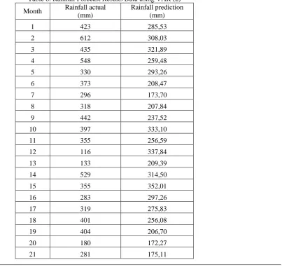
Validation of VAR Model
Forecasting is not the only final goal in a time series model, but many argue that forecasting is an inseparable part of many time series models. To determine the accuracy of forecasting the VAR model used the mean absolute percentage error (MAPE) value of the model for the rainfall variables. The results of rainfall forecast for the last 2 years 2016-2017 are presented in table 8.
Table 8. Rainfall Forecast Results Data using VAR (2)
Month Rainfall actual (mm)
Rainfall prediction (mm)
1 423 285,53
2 612 308,03
3 435 321,89
4 548 259,48
5 330 293,26
6 373 208,47
7 296 173,70
8 318 207,84
9 442 237,52
10 397 333,10
11 355 256,59
12 116 337,84
13 133 209,39
14 529 314,50
15 355 352,01
16 283 297,26
17 319 275,83
18 401 256,08
19 404 206,70
20 180 172,27
102
Copyright © 2018. IJEMR. All Rights Reserved.
22 333 281,45
23 206 369,64
24 180 359,35
MAPE 42,18
Based on table 3, obtained MAPE value for rainfall of 42.18. The MAPE value obtained is relatively large. There are several things that cause large MAPE value, such as rainfall data used for modeling has high fluctuations and from modeling only humidity and temperature variables that have a significant effect on rainfall.
V.
CONCLUSIONS AND
RECOMMENDATIONS
Conclusions
Based on the results obtained VAR model for elements of rainfall weather, air humidity, air temperature, air pressure, wind direction and speed. For the VAR model the rainfall variables in the t-month are affected by the t-1 moisture air moisture, the t-2 moisture air and the air temperature at t-2.
The VAR model (2) used is used to forecast the next period. MAPE values obtained are influenced by several things such as rainfall data used for modeling has high fluctuations, and many other variables that have significant effect on rainfall.
REFERENCES
[1] Arpan F, Kirono GDC & Sudjarwadi. (2004). Kajian meteorologis hubungan antara hujan harian dan unsur-unsur cuaca studi kasus di stasiun meteorologi adisucipto yogyakarta. Majalah Geografi Indonesia, 2, 69-79. [2] Boer R. (2003). Penyimpangan iklim di Indonesia. makalah seminar nasional ilmu tanah. Yogyakarta, KMIT
Jurusan Tanah Fakultas Pertanian UGM. Yogyakarta.
[3] Ender W. (1995). Applied Econometric Time Series. New York: Willey and sons. Inc.
[4] Fisher NI. (1993). Statistical analysis of circular data. Cambridge: Cambridge University Press.
[5] Hadi YS. (2003). Analisis vector autoregressive (VAR) terhadap korelasi antara pendapatan nasional dan
investasi pemerintah di Indonesia 1983/1984-1999/2000.
Jurnal Keuangan dan Moneter, 2, 107-121.
[6] Naylor, L.N., W.P. Falcon, D. Rochberg, & N. Wada. (2001). Using el niño/southern oscillation climate data to predict rice production in Indonesia. Climatic Change, 50(3), 255-265.
[7] Jammalamadaka SR & Sengupta A. (2001). Topics in circular statistics (Series on multivariate analysis). Singapore: World Scientific.
[8] Huffman, G.J., R.F. Adler, D.T. Bolvin, G. Gu, E.J. Nelkin, K.P. Bowman, Y. Hong, E.F. Stocker, & D.B. Wolff. (2007). The TRMM multisatellite precipitation analysis (TMPA): Quasi-global, multiyear, combined-sensor precipitation estimates at fine scales. Journal of Hydrometeorology, 8(1), 38-55.
[9] Mardia KV, Peter EJ. (1972). Directional statistics. New York: Willey and sons. Ltd.
[10] Lutkepohl H. 1993. Introduction to multiple time series analysis. Verlag: Springer- Verlag.
[11] Gujarati, Damodar N. (2006). Essential of
econometrics. New York: McGraw-Hill Co.
[12] Adi Nugroho, Sri Hartati, Subanar, & Khabib Mustofa. (2014). Vector Autoregression (Var) model for rainfall forecast and isohyet mapping in semarang – central java–Indonesia. International Journal of Advanced Computer Science and Applications, 5(11), 44-49.
[13] Sims, C. A., & Zha, T. (1998). Bayesian methods for dynamic multivariate models. International
Economic Review, 39(4), 949- 968.
[14] Sandi IM. (1987). Iklim regional Indonesia. Depok: UI Jurusan Geografi.
[15] SAS Institut Inc. (1996). Forecasting examples for business and economics using the SAS system. North Carolina, USA: SAS Intitut Inc.
[16] Subarna D. (2009). Aplikasi jaringan neural untuk pemodelan dan prediksi curah hujan. Berita Dirgantara,
1, 13-18.