Robust Optimization over Multiple Domains

The Thirty-Third AAAI Conference on Artificial Intelligence (AAAI-19)

Robust Optimization over Multiple Domains

Qi Qian, Shenghuo Zhu, Jiasheng Tang, Rong Jin, Baigui Sun, Hao Li

{qi.qian, shenghuo.zhu, jiasheng.tjs, jinrong.jr, baigui.sbg, lihao.lh}@alibaba-inc.com

Abstract

In this work, we study the problem of learning a single model for multiple domains. Unlike the conventional machine learn-ing scenario where each domain can have the correspondlearn-ing model, multiple domains (i.e., applications/users) may share the same machine learning model due to maintenance loads in cloud computing services. For example, a digit-recognition model should be applicable to hand-written digits, house numbers, car plates, etc. Therefore, an ideal model for cloud computing has to perform well at each applicable domain. To address this new challenge from cloud computing, we de-velop a framework of robust optimization over multiple do-mains. In lieu of minimizing the empirical risk, we aim to learn a model optimized to the adversarial distribution over multiple domains. Hence, we propose to learn the model and the adversarial distribution simultaneously with the stochastic algorithm for efficiency. Theoretically, we analyze the con-vergence rate for convex and non-convex models. To our best knowledge, we first study the convergence rate of learning a robust non-convex model with a practical algorithm. Further-more, we demonstrate that the robustness of the framework and the convergence rate can be further enhanced by appro-priate regularizers over the adversarial distribution. The em-pirical study on real-world fine-grained visual categorization and digits recognition tasks verifies the effectiveness and ef-ficiency of the proposed framework.

Introduction

Learning a single model for multiple domains becomes a fundamental problem in machine learning and has found ap-plications in cloud computing services. Cloud computing witnessed the development of machine learning in recent years. Apparently, users of these cloud computing services can benefit from sophisticated models provided by service carrier, e.g., Aliyun. However, the robustness of deployed models becomes a challenge due to the explosive popular-ity of the cloud computing services. Specifically, to main-tain the scalability of the cloud computing service, only a

singlemodel will exist in the cloud for the same problem from different domains. For example, given a model for dig-its recognition in cloud, some users may call it to identify the handwritten digits while others may try to recognize the printed digits (e.g., house number).

Copyright c2019, Association for the Advancement of Artificial Intelligence (www.aaai.org). All rights reserved.

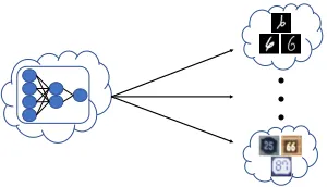
Figure 1: Illustration of optimizing over multiple domains. In this example, a digit-recognition model provided by cloud service carrier should be applicable for multiple domains, e.g., handwritten digits, printed digits.

A satisfied model has to deal with both domains (i.e., handwritten digits, printed digits) well in the modern ar-chitecture of cloud computing services. This problem is il-lustrated in Fig. 1. Note that the problem is different from multi-task learning (Zhang and Yang 2017) that aims to learn different models (i.e., multiple models) for different tasks by exploiting the shared information between related tasks.

meth-ods with non-convex loss functions, e.g, deep neural net-works (He et al. 2016; Krizhevsky, Sutskever, and Hinton 2012; Szegedy et al. 2015). (Chen et al. 2017) proposed an algorithm to solve the non-convex problem, but their anal-ysis relies on a near-optimal oracle for the non-convex sub-problem, which is not feasible for most non-convex prob-lems in real tasks. Besides, their algorithm has to go through the whole data set at least once to update the parameters at every iteration, which makes it too expensive for the large-scale data set.

In this work, we propose a framework to learn a ro-bust model over multiple domains rather than examples. By learning the model and the adversarial distribution simulta-neously, the algorithm can balance the performance between different domains adaptively. Compared with the previous work, the empirical data distribution in each domain remains unchanged and our framework only learns the distribution over multiple domains. Therefore, the learned model will not be potentially misled by the adversarial distribution over ex-amples. Our framework is also comparatively efficient due to the adoption of stochastic gradient descent (SGD) for op-timization. More importantly, we first prove that the pro-posed method converges with a rate ofO(1/T1/3)without the dependency on the oracle. To further improve the ro-bustness of the framework, we introduce a regularizer for the adversarial distribution. We find that an appropriate reg-ularizer not only prevents the model from a trivial solution but also accelerates the convergence rate toO(plog(T)/T). The detailed theoretical results are summarized in Table 1. The empirical study on pets categorization and digits recog-nition demonstrates the effectiveness and efficiency of the proposed method.

Table 1: Convergence rate for the non-convex model and ad-versarial distribution (“Adv-Dist”) under different settings.

Setting Convergence

Model Adv-Dist Model Adv-Dist Smooth Concave O( 1

T1/3) O(

1

T1/3)

Smooth Strongly Concave O(

q

log(T)

T ) O(

log(T)

T )

Related Work

Robust optimization has been extensively studied in the past decades (Bertsimas, Brown, and Caramanis 2011). Recently, it has been investigated to improve the performance of the model in the worst case data distribution, which can be in-terpreted as regularizing the variance (Duchi, Glynn, and Namkoong 2016). For a set of convex loss functions (e.g., a single data set), (Namkoong and Duchi 2016) and (Shalev-Shwartz and Wexler 2016) proposed to optimize the maxi-mal loss, which is equivalent to minimizing the loss with the worst case distribution generated from the empirical distri-bution of data. (Namkoong and Duchi 2016) showed that for thef-divergence constraint, a standard stochastic mirror de-scent algorithm can converge at the rate ofO(1/√T)for the convex loss. In (Shalev-Shwartz and Wexler 2016), the anal-ysis indicates that minimizing the maximal loss can improve

the generalization performance. In contrast to a single data set, we focus on dealing with multiple data sets and propose to learn the non-convex model in this work.

To tackle non-convex losses, (Chen et al. 2017) proposed to apply a near-optimal oracle. At each iteration, the oracle is called to return a near-optimal model for the given dis-tribution. After that, the adversarial distribution over exam-ples is updated according to the model from the oracle. With anα-optimal oracle, authors proved that the algorithm can converge to theα-optimal solution at the rate ofO(1/√T), whereT is the number of iterations. The limitation is that even if we assume a near-optimal oracle is accessible for the non-convex problem, the algorithm is too expensive for the real-world applications. It is because that the algorithm has to enumerate the whole data set to update the param-eters at each iteration. Without a near-optimal oracle, we prove that the proposed method can converge with a rate ofO(plog(T)/T)with an appropriate regularizer and the computational cost is much cheaper.

Robust Optimization over Multiple Domains

an image) andyk

i is the corresponding label. We aim to learn

a model that performs well over all domains. It can be cast as a robust optimization problem as follows.

min

W

s.t. ∀k, fk(W)≤

whereW is the parameter of a prediction model.fk(·)is the

empirical risk of thek-th domain as

fk(W) = X

i:xk

i∈Sk

1

|Sk|

`(xk_i, y_ik;W)

and `(·) can be any non-negative loss function. Since the cross entropy loss is popular in deep learning, we will adopt it in the experiments.

The problem is equivalent to the following minimax prob-lem

min

W pmax:p∈∆L(p, W) =p

>_{f(W) (1)}

wheref(W) = [f1(W),· · · , fK(W)]>.pis an adversarial

distribution over multiple domains andp∈ ∆, where∆is the simplex as∆ ={p∈_RK_|PK

k=1pk = 1;∀k, pk ≥0}.

It is a game between the prediction model and the adver-sarial distribution. The minimax problem can be solved in an alternating manner, which applies gradient descent to learn the model and gradient ascent to update the adversarial dis-tribution. Considering the large number of examples in each data set, we adopt SGD to observe an unbiased estimation for the gradient at each iteration, which avoids enumerating the whole data set. Specifically, at thet-th iteration, a mini-batch of sizemis randomly sampled from each domain. The loss of the mini-batch from thek-th domain is

ˆ

f_kt(W) = 1

m m

X

i=1

It is apparent thatE[ ˆf_kt(W)] =fk(W)andE[∇fˆ_kt(W)] =

∇fk(W).

Algorithm 1Stochastic Algorithm for Robust Optimization

Input: Data set {S1,· · · , SK}, size of mini-batch m, step-sizesηw,ηp

Initializep1= [1/K,· · ·,1/K]

fort= 1toT do

Randomly samplemexamples from each domain UpdateWt+1as in Eqn. 2

Updatept+1as in Eqn. 3

end for return W = 1

T

P

tWt,p¯= _T1 Ptpt

After sampling, we first update the model by gradient de-scent as

Wt+1=Wt−ηwˆgt; where gtˆ = X

k

ptk∇fˆkt(Wt) (2)

Then, the distributionpis updated in an adversarial way. Since p is from the simplex, we can adopt multiplicative updating criterion (Arora, Hazan, and Kale 2012) to update it as

pk_t+1 =p

k

texp(ηpfˆkt(Wt))

Zt ;

where Zt=

X

k

pk_texp(ηpfˆkt(Wt)) (3)

Alg. 1 summarizes the main steps of the approach. For the convex loss functions, the convergence rate is well known (Nemirovski et al. 2009) and we provide a high prob-ability bound for completeness. All detailed proofs of this work can be found in the supplementary.

Lemma 1. Assume the gradient ofW and the function value are bounded as∀t,k∇fˆ_kt(Wt)kF ≤σ,kˆft(Wt)k2≤γand ∀W, kWkF ≤ R. Let(W ,p¯)denote the results returned by Alg. 1 afterT iterations. Set the step-sizes asηw= R

σ√T and ηp = 2

√ 2 log(K)

γ√T . Then, with a probability1−δ, we have

max

p L(p, W)−minW L(¯p, W)≤

c1 √

T +

2c2 p

log(2/δ)

√

T

wherec1=O( p

log(K))andc2is a constant.

Lemma 1 shows that the proposed method with the con-vex loss can converge to the saddle point at the rate of O(1/√T)with high probability, which is a stronger result than the expectation bound in (Namkoong and Duchi 2016). Note that settingηw=O(√1

T)andηp=O(

q log(K)

T )will

not change the order of the convergence rate, which means

σ,γandRare not required for implementation.

Non-convexity

Despite the extensive studies about the convex loss, there is little research about the minimax problem with non-convex loss. To provide the convergence rate for the non-convex problem, we first have the following lemma.

Lemma 2. With the same assumptions as in Lemma 1, if`(·)

is non-convex butL-smoothness, we have

X

t

E[k∇WtL(pt, Wt)k

2

F]≤

L(p0, W0)

ηw +

ηpT γ2

2ηw +

T Lηwσ2

2

X

t

E[L(pt, Wt)]≥max

p∈∆

X

t

E[L(p, Wt)]−(log(K)

ηp +

T ηpγ2

8 )

Since the loss is non-convex, the convergence is measured by the norm of the gradient (i.e., stationary point), which is a standard criterion for the analysis in the non-convex prob-lem (Ghadimi and Lan 2013). Lemma 2 indicates that W

can converge to a stationary point where pt is a qualified

adversary by setting the step-sizes elaborately. Furthermore, it demonstrates that the convergence rate ofWwill be influ-enced by the convergence rate ofpviaηp.

With Lemma 2, we have the convergence analysis of the non-convex minimax problem as follows.

Theorem 1. With the same assumptions as in Lemma 2, if

we set the step-sizes asηw=

q

2γ√2 log(K)

σ√L T

−1/3_andη

p=

2√2 log(K)

γ T

−2/3_{, we have}

E[1

T

X

t

k∇WtL(pt, Wt)k

2

F]

≤(_qL(p0, W0) 2γp2 log(K)

+

q

2γp2 log(K))σ√LT−1/3

E[1

T

X

t

L(pt, Wt)]

≥E[max

p∈∆

1

T

X

t

L(p, Wt)]−γ p

log(K)

√

2 T

−1/3

Remark Compared with the convex case in Lemma 1, the convergence rate of a non-convex problem is degraded from O(1/√T)toO(1/T1/3). It is well known that the conver-gence rate of general minimization problems with a smooth non-convex loss can be up toO(1/√T)(Ghadimi and Lan 2013). Our results further demonstrate that minimax prob-lems with non-convex loss is usually harder than non-convex minimization problems.

Different step-sizes can lead to different convergence rates. For example, if the step-size for updating p is in-creased asηp = 1/

√

T and that for model is decreased as

ηw= 1/T1/4, the convergence rate ofpcan be accelerated

toO(1/√T)while the convergence rate ofWwill degener-ate toO(1/T1/4_{). Therefore, if a sufficiently small step-size} is applicable forp, the convergence rate ofW can be sig-nificantly improved. We exploit this observation to enhance the convergence rate in the next subsection.

Regularized Non-convex Optimization

Eqn. 1 (i.e., one-hot value in p). Besides the issue of ro-bustness, it is prevalent in real-world applications that the importance of domains is different according to their bud-gets, popularity, etc. Incorporating the side information into the formulation is essential for the success in practice. Given a prior distribution, the problem can be written as

min

W pmax:p∈∆p

>_f(W)

s.t. D(p||q)≤τ

whereqis the prior distribution which can be a distribution defined from the side information or a uniform distribution for robustness.D(·)defines the distance between two distri-butions, e.g.,Lpdistance orKL-divergence

DL2(p||q) =kp−qk

2

2; DKL(p||q) = X

k

pklog(pk/qk)

Since KL-divergence cannot handle the prior distribution with zero elements, optimal transportation (OT) distance be-comes popular recently to overcome the drawback

DOT(p||q) = min

P∈U(p,q)hP, Mi

For computational efficiency, we use the version with an en-tropy regularizer (Cuturi 2013) and we have

Proposition 1. Define theOTregularizer as

DOT(p||q) = max

α,β minP

1

ν

X

i,j

Pi,jlog(P(i, j))

+Pi,jMi,j+α>(P1K−p) +β>(P1K−q) (4) and it is convex inp.

According to the duality theory (Boyd and Vandenberghe 2004), for eachτ, we can have the equivalent problem with a specifiedλ

min

W pmax:p∈∆ ˆ

L(p, W) =p>f(W)−λ

2D(p||q) (5)

Compared with the formulation in Eqn. 1, we introduce a regularizer for the adversarial distribution.

If D(p||q) is convex in p, the similar convergence as in Theorem. 1 can be obtained with the same analysis. Moreover, according to the research for SGD, the strongly convexity is the key to achieve the optimal convergence rate (Rakhlin, Shamir, and Sridharan 2012). Hence, we adopt a strongly convex regularizer i.e.,L2 regularizer, for the distribution. The convergence rate for other strongly con-vex regularizers can be obtained with a similar analysis by defining the smoothness and the strongly convexity with the corresponding norm.

Equipped with theL2regularizer, the problem in Eqn. 5 can be solved with projected first-order algorithm. We adopt the projected gradient ascent to update the adversarial distri-bution as

pt+1=P∆(pt+ηtpˆht); where ˆht= ˆft−λ(pt−q)

P∆(p)projects the vectorponto the simplex. The projec-tion algorithm can be found in (Duchi et al. 2008) which is based onK.K.T.condition. We also provide the gradient of

OTregularizer in the supplementary.

Since the regularizer (i.e.,−L2) is strongly concave, the convergence of p can be accelerated dramatically, which leads to a better convergence rate for the minimax problem. The theoretical result is as follows.

Theorem 2. With the same assumptions as in Theorem 1, if we assume ∀t, kˆht_k

2 ≤ µand set step-sizes as ηw = 2µ√log(T)

σ√λLT andη t

p= λt1, we have

E[1

T X

t

k∇WtLˆ(pt, Wt)k

2

F]

≤ L(p0, W0)σ

√ λL

2µplog(T) +

µπ2_σ√_λL

12 + 2µσ

p

λLlog(T)

!

1

√ T

E[1

T X

t

ˆ

L(pt, Wt)]≥E[max

p∈∆

1

T X

t

ˆ

L(p, Wt)]−µ

2_log(T)

λT

Remark With the strongly concave regularizer, it is not surprise to obtain theO(log(T)/T)convergence rate forp. As we discussed in Lemma 2, a fast convergence rate ofp

can improve that ofW. In Theorem 2, the convergence rate of W is improved from O(1/T1/3_)toO(p

log(T)/T). It shows that the applied regularizer not only improves the ro-bustness of the proposed framework but also accelerates the learning procedure.

Moreover, the step-size for the adversarial distribution provides a trade-off between the bias and variance of the gradient. Therefore, the convergence rate can be further im-proved by reducing the variance. We shrink the gradient with a factorcand update the distribution as

pt+1=P∆(pt+

ηt p

1 +c/t

ˆ

ht)

When takingηpt= λt1, the update becomes

pt+1=P∆(pt+

1

λ(t+c) ˆ

ht) (6)

With a similar analysis as Theorem 2, we have

Theorem 3. With the same assumptions as in Theorem 2, if we set the step-sizeηt_p=_λ(t1_+c), we have

E[1

T X

t

ˆ

L(pt, Wt)]

≥E[max

p∈∆

1

T X

t

ˆ

L(p, Wt)]−(λc+µ

2

2λln( T

c + 1) +

µ2

2λ)

1

T

It shows that the constantccan control the trade-off be-tween bias (i.e., λc) and variance (i.e., µ_2λ2ln(T_c + 1)). By setting the constant appropriately, we can have the follow-ing corollary

Corollary 1. When settingc= µ2

λ2₍₁₊q₁₊2µ2

λ2T)

, the RHS in

Theorem 3 is maximum.

The optimality is from the fact that RHS is concave inc

Algorithm 2Stochastic Regularized Robust Optimization

Input: Data set {S1,· · · , SK}, size of mini-batch m, step-sizesηw,ηp

Initializep1= [1/K,· · ·,1/K]

Compute the constantcas in Corollary 1

fort= 1toT do

Randomly samplemexamples from each domain UpdateWt+1with gradient descnet

(Optional) Solve the problem in Eqn. 4 if applying DOT(pt||q)

Updatept+1with gradient ascent Projectpt+1onto the simplex

end for

Trade Efficiency for Convergence

In this subsection, we study if we can recover the optimal convergence rate for the general non-convex problem as in (Ghadimi and Lan 2013). Note that (Chen et al. 2017) ap-plies a near-optimal oracle to achieve the O(1/√T) con-vergence rate. Given a distribution, it is hard to observe an oracle for the non-convex model. In contrast, obtaining the near-optimal adversarial distribution with a fixed model is feasible. For the original problem in Eqn. 1, the solu-tion is trivial as returning the index of the domain with the largest empirical loss. For the problem with the regularizer in Eqn. 5, the near-optimal p can be obtained efficiently by any first order methods (Boyd and Vandenberghe 2004). Therefore, we can change the updating criterion for the dis-tribution at thet-th iteration to

Obtainpt+1such thatkpt+1−p∗t+1k1≤ξt+1 where p∗t+1= arg max

p:p∈∆L(p, Wt) (7)

With the new updating criterion and letting F(W) = maxpL(p, W), we can have a better convergence rate as

follows.

Theorem 4. With the same assumptions as in Theorem 1, if we updatepas in Eqn. 7, whereξt = √1

t, and set the step-size asηw=

√

2

σ√LT, we have

X

t E[1

Tk∇F(Wt)k

2

F]≤(F(W0) + 1) √

Lσ

√

2T +

2σ2 √

T

For the problem in Eqn. 1,ξt can be0by a single pass through the whole data set. It shows that with an expen-sive but feasible operator as in Eqn. 7, the proposed method can recover the optimal convergence rate for the non-convex problem.

Experiments

We conduct the experiments on training deep neural net-works over multiple domains. The methods in the compari-son are summarized as follows.

• Individual: It learns the model from an individual do-main.

• MixtureEven: It learns the model from multiple domains with even weights, which is equivalent to fixingpas an uniform distribution.

• MixtureOpt: It implements the approach proposed in Alg. 2 that learns the model and the adversarial distribu-tion over multiple domains simultaneously.

We adopt the popular cross entropy loss as the loss func-tion `(·)in this work. Deep models are trained with SGD and the size of each mini-batch is set to200. For the meth-ods learning with multiple domains, the number of exam-ples from different domains are the same in a mini-batch and the size is m = 200/K. Compared with the strat-egy that samples examples according to the learned dis-tribution, the applied strategy is deterministic and will not introduce extra noise. The method is evaluated by inves-tigating the worst case performance among multiple do-mains. For the worst case accuracy, it is defined asAccw=

mink{Acc1,· · ·,AccK}. The worst case loss is defined as fw(W) = maxk{f1(W),· · · , fK(W)}. All experiments are implemented on an NVIDIA Tesla P100 GPU.

Pets Categorization

First, we compare the methods on a fine-grained vi-sual categorization task. Given the data sets of VGG cats&dogs (Parkhi et al. 2012) and ImageNet (Russakovsky et al. 2015), we extract the shared labels between them and then generate the subsets with desired labels from them, respectively. The resulting data set consists of 24 classes and the task is to assign the image of pets to one of these classes. For ImageNet, each class contains about1,200 im-ages for training while that of VGG only has100 images. Therefore, we apply data augmentation by flipping (hori-zontal+vertical) and rotating ({45◦,· · ·,315◦}) for VGG to avoid overfitting. After that, the number of images in VGG is similar to that of ImageNet. Some exemplar images from these data sets are illustrated in Fig. 3. We can find that the task in ImageNet is more challenging than that in VGG due to complex backgrounds.

We adopt ResNet18 (He et al. 2016) as the base model in this experiment. It is initialized with the parameters learned from ILSVRC2012 (Russakovsky et al. 2015) and we set the learning rate asηw = 0.005 for fine-tuning.

Consider-ing the small size of data sets, we also include the method of (Chen et al. 2017) in comparison and it is denoted as

MixtureOracle. Since the near-optimal oracle is infeasible forMixtureOracle, we apply the model with100SGD iter-ations instead as suggested in (Chen et al. 2017). The prior distribution in the regularizer is set to the uniform distribu-tion.

500 1000 1500 2000 2500 3000 3500 4000 4500 5000 Number of Mini-batches 0

0.2 0.4 0.6 0.8 1 1.2 1.4 1.6 1.8 2

Worst Case Training Loss

Individual ImageNet

Individual VGG

Mixture Opt

(a) Pets Categorization

500 1000 1500 2000 2500 3000 3500 4000 4500 5000

Number of Mini-batches 0

0.2 0.4 0.6 0.8 1 1.2 1.4 1.6 1.8 2

Worst Case Training Loss

Mixture Even

Mixture Oracle

Mixture Opt

(b) Pets Categorization

1 2 3 4 5 6

Number of Mini-batches #104 0

0.5 1 1.5 2 2.5 3 3.5 4 4.5

Worst Case Training Loss

Individual MNIST

Individual SVHN

Mixture Opt

(c) Digits Recognition

1 2 3 4 5 6

Number of Mini-batches #104

0 0.5 1 1.5 2 2.5

Worst Case Training Loss

Mixture Even

Mixture Opt

(d) Digits Recognition

Figure 2: Illustration of worst case training loss.

Table 2: Comparison on pets categorization. We report the loss and accuracy (%) on each data set.

Methods ImageNet_Loss VGG AccTrw AccTew

Tr AccTr AccTe LossTr AccTr AccTe

IndividualImageNet 0.07 98.95 89.92 0.85 74.56 80.44 74.56 80.44 IndividualVGG 0.90 75.47 77.92 0.02 100.00 86.85 75.47 77.92 MixtureEven 0.17 95.56 88.50 0.05 99.58 89.85 95.56 88.50 MixtureOracle 0.15 96.04 88.92 0.06 99.41 89.99 96.04 88.92 MixtureOpt 0.12 97.36 89.42 0.11 97.72 89.35 97.36 89.35

VGG

ImageNet

Figure 3: Exemplar images from ImageNet and VGG.

500 1000 1500 2000 2500 3000 3500 4000 4500 5000

Number of Mini-batches -0.2

-0.15 -0.1 -0.05 0 0.05 0.1 0.15

Difference in Training Loss

Mixture Even Mixture Oracle Mixture Opt

Figure 4: Comparison of discrepancy in losses.

1 2 3 4

0 2000 4000 6000 8000 10000 12000

Running Time (seconds)

Mixture Even

Mixture Opt

Mixture OT

Mixture Oracle

Figure 5: Comparison of running time.

the results of the methods learning with multiple data sets. First, we find that both MixtureOracleand MixtureOpt can achieve the lower worst case loss than MixtureEven, which

500 1000 1500 2000 2500 3000 3500 4000 4500 5000

Number of Mini-batches

0 0.2 0.4 0.6 0.8 1 1.2 1.4 1.6 1.8 2

Training Loss

Mixture Even-Best Mixture Even-Worst Mixture Opt-Best Mixture Opt-Worst

(a)σ∈ {0,4,8,12}

500 1000 1500 2000 2500 3000 3500 4000 4500 5000

Number of Mini-batches

0 0.5 1 1.5 2 2.5 3

Training Loss

Mixture Even-Best Mixture Even-Worst Mixture Opt-Best Mixture Opt-Worst

(b)σ∈ {0,10,20,30}

Figure 6: Illustration of best and worst training loss on Ima-geNet with Gaussian noiseN(0, σ2).

confirms the effectiveness of the robust optimization. Sec-ond, MixtureOptperforms best among all of these methods and it demonstrates that the proposed method can optimize the performance over the adversarial distribution. To inves-tigate the discrepancy between the performances on two do-mains, we illustrate the result in Fig. 4. The discrepancy is measured by the difference between the empirical loss as

fImageNet−fVGG. We can find that fImageNet is smaller thanfVGGat the beginning butfVGGdecreases faster than

perfor-500 1000 1500 2000 2500 3000 3500 4000 4500 5000 Number of Mini-batches -0.08

-0.06 -0.04 -0.02 0 0.02 0.04 0.06

Difference in Training Loss 6=0.1 6=0.05 6=0.01

(a)DL2(p||q)

500 1000 1500 2000 2500 3000 3500 4000 4500 5000

Number of Mini-batches

-0.6 -0.4 -0.2 0 0.2 0.4 0.6 0.8

Difference in Distribution

6=0.1 6=0.05 6=0.01

(b)DL2(p||q)

500 1000 1500 2000 2500 3000 3500 4000 4500 5000

Number of Mini-batches

-0.2 -0.15 -0.1 -0.05 0 0.05 0.1 0.15

Difference in Training Loss 6=0.001

6=0.0005

6=0.0001

(c)DOT(p||q)

500 1000 1500 2000 2500 3000 3500 4000 4500 5000

Number of Mini-batches

-1 -0.8 -0.6 -0.4 -0.2 0 0.2 0.4 0.6

Difference in Distribution

6=0.001 6=0.0005 6=0.0001

(d)DOT(p||q)

Figure 7: Illustration of the influence of the regularizer. Table 3: Comparison on digits recognition.

Methods MNIST_Loss SVHN AccTrw AccTew

Tr AccTr AccTe LossTr AccTr AccTe

IndividualMNIST 0.001 100.00 98.81 4.01 30.80 29.58 30.80 29.58 IndividualSVHN 1.91 66.66 68.25 0.10 97.11 91.84 66.66 68.25 MixtureEven 0.001 100.00 98.74 0.14 96.20 91.33 96.20 91.33 MixtureOpt 0.03 99.03 98.13 0.11 97.05 92.14 97.05 92.14

mance between them.

To further demonstrate that MixtureOptcan trade the per-formance effectively, we conduct the experiments with noisy data. We simulate each individual domain by adding the ran-dom Gaussian noise fromN(0, σ2)to each pixel of the im-ages from ImageNet pets. We vary the variance to generate the different domains and obtain two tasks where each has four domains withσ∈ {0,4,8,12}andσ∈ {0,10,20,30}, respectively. Fig. 6 compares the gap between the best and worst performance on different domains for MixtureEven and MixtureOpt. First, we can find that the proposed method improves the worst-case performance significantly while keeping the best performance almost the same. Besides, do-mains can achieve the similar performance for the simple task with variance in{0,4,8,12}. For the hard task that in-cludes an extreme domain with noise from N(0,302), the best performance is not sacrificed much due to the appropri-ate regularizer in MixtureOpt.

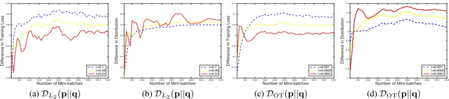
After the comparison of performance, we illustrate the in-fluence of the parameterλin Fig. 7. The parameter can be found in Eqn. 5 and it constrains the distance of the adversar-ial distribution to the prior distribution. Besides theL2 regu-larizer applied in MixtureOpt, we also include the results of theOTregularizer defined in Proposition 1 and the method is denoted asMixtureOT. Fig. 7 (a) and (c) compare the dis-crepancy between the losses as in previous experiments. It is obvious that the smaller theλ, the smaller the gap between two domains. Fig. 7 (b) and (d) summarize the drifting in a distribution, which is defined aspImageNet−pVGG. Evi-dently, the learned adversarial distribution can switch adap-tively according to the performance of the current model and the importance of multiple domains can be constrained well by settingλappropriately.

Finally, we compare the running time in Fig. 5. Due to the lightweight update for the adversarial distribution, MixtureOpt and MixtureOThave almost the same running

time as MixtureEven. MixtureOracle has to enumerate the whole data set after each100SGD iterations to update the current distribution, hence, its running time with only 50

complete iterations is nearly 3 times slower than the pro-posed method with5,000iterations on these small data sets.

Digits Recognition

In this experiment, we examine the methods on the task of digits recognition, which is to identify 10 digits (i.e.,

0-9) from images. There are two benchmark data sets for the task: MNIST and SVHN. MNIST (LeCun et al. 1998) is collected for recognizing handwritten digits. It contains

60,000 images for training and 10,000 images for test. SVHN (Netzer et al. 2011) is for identifying the house num-bers from Google Street View images, which consists of

604,388training images and26,032test images. Note that the examples in MNIST are28×28gray images while those in SVHN are 32×32 color images. To make the format consistent, we resize images in MNIST to be 32×32and repeat the gray channel in RGB channels to generate the color images. Considering the task is more straightforward than pets categorization, we apply the AlexNet (Krizhevsky, Sutskever, and Hinton 2012) as the base model in this ex-periment and set the learning rate as ηw = 0.01. With a different deep model, we also demonstrate that the proposed framework can incorporate with various deep models.

Conclusion

In this work, we propose a framework to learn a robust model over multiple domains, which is essential for the ser-vice of cloud computing. The introduced algorithm can learn the model and the adversarial distribution simultaneously, for which we provide a theoretical guarantee on the conver-gence rate. The empirical study on real-world applications confirms that the proposed method can obtain a robust non-convex model. In the future, we plan to examine the per-formance of the method with more applications. Besides, extending the framework to multiple domains with partial overlapped labels is also important for real-world applica-tions.

Acknowledgments

We would like to thank Dr. Juhua Hu from University of Washington Tacoma and anonymous reviewers for their valuable suggestions that help to improve this work.

References

Arora, S.; Hazan, E.; and Kale, S. 2012. The multiplicative weights update method: a meta-algorithm and applications.

Theory of Computing8(1):121–164.

Bertsimas, D.; Brown, D. B.; and Caramanis, C. 2011. The-ory and applications of robust optimization. SIAM Review

53(3):464–501.

Boyd, S., and Vandenberghe, L. 2004.Convex optimization. Cambridge university press.

Chen, R. S.; Lucier, B.; Singer, Y.; and Syrgkanis, V. 2017. Robust optimization for non-convex objectives. InNIPS, 4708–4717.

Cuturi, M. 2013. Sinkhorn distances: Lightspeed computa-tion of optimal transport. InNIPS, 2292–2300.

Duchi, J. C.; Shalev-Shwartz, S.; Singer, Y.; and Chandra, T. 2008. Efficient projections onto thel_{1-ball for learning}

in high dimensions. InICML, 272–279.

Duchi, J. C.; Glynn, P.; and Namkoong, H. 2016. Statis-tics of Robust Optimization: A Generalized Empirical Like-lihood Approach.ArXiv e-prints.

Ghadimi, S., and Lan, G. 2013. Stochastic first- and zeroth-order methods for nonconvex stochastic program-ming. SIAM Journal on Optimization23(4):2341–2368. He, K.; Zhang, X.; Ren, S.; and Sun, J. 2016. Deep residual learning for image recognition. InCVPR, 770–778. Krizhevsky, A.; Sutskever, I.; and Hinton, G. E. 2012. Imagenet classification with deep convolutional neural net-works. InNIPS, 1106–1114.

LeCun, Y.; Bottou, L.; Bengio, Y.; and Haffner, P. 1998. Gradient-based learning applied to document recognition.

Proceedings of the IEEE86(11):2278–2324.

Namkoong, H., and Duchi, J. C. 2016. Stochastic gradi-ent methods for distributionally robust optimization with f-divergences. InNIPS, 2208–2216.

Nemirovski, A.; Juditsky, A.; Lan, G.; and Shapiro, A. 2009. Robust stochastic approximation approach to stochastic pro-gramming. SIAM Journal on Optimization 19(4):1574– 1609.

Netzer, Y.; Wang, T.; Coates, A.; Bissacco, A.; Wu, B.; and Ng, A. Y. 2011. Reading digits in natural images with unsu-pervised feature learning. InNIPS workshop on deep learn-ing and unsupervised feature learnlearn-ing, volume 2011, 5. Parkhi, O. M.; Vedaldi, A.; Zisserman, A.; and Jawahar, C. V. 2012. Cats and dogs. InCVPR.

Rakhlin, A.; Shamir, O.; and Sridharan, K. 2012. Making gradient descent optimal for strongly convex stochastic op-timization. InICML.

Russakovsky, O.; Deng, J.; Su, H.; Krause, J.; Satheesh, S.; Ma, S.; Huang, Z.; Karpathy, A.; Khosla, A.; Bernstein, M.; Berg, A. C.; and Fei-Fei, L. 2015. ImageNet Large Scale Visual Recognition Challenge. IJCV115(3):211–252. Shalev-Shwartz, S., and Wexler, Y. 2016. Minimizing the maximal loss: How and why. InICML, 793–801.