Inference via Low-Dimensional Couplings

(1)

Inference via Low-Dimensional Couplings

Massachusetts Institute of Technology Cambridge, MA 02139 USA

Editor:Manfred Opper

Abstract

We investigate the low-dimensional structure of deterministic transformations between random variables, i.e., transport maps between probability measures. In the context of statistics and machine learning, these transformations can be used to couple a tractable “reference” measure (e.g., a standard Gaussian) with a target measure of interest. Direct simulation from the desired measure can then be achieved by pushing forward reference samples through the map. Yet characterizing such a map—e.g., representing and evaluat-ing it—grows challengevaluat-ing in high dimensions. The central contribution of this paper is to establish a link between the Markov properties of the target measure and the existence of low-dimensional couplings, induced by transport maps that aresparseand/ordecomposable. Our analysis not only facilitates the construction of transformations in high-dimensional settings, but also suggests new inference methodologies for continuous non-Gaussian graph-ical models. For instance, in the context of nonlinear state-space models, we describe new variational algorithms for filtering, smoothing, and sequential parameter inference. These algorithms can be understood as the natural generalization—to the non-Gaussian case—of the square-root Rauch–Tung–Striebel Gaussian smoother.

Keywords: transport map, variational inference, graphical models, sparsity, state-space models, joint parameter and state estimation

1. Introduction

This paper studies the low-dimensional structure of transformations between random vari-ables. Such transformations, which can be understood as transport maps between prob-ability measures, are ubiquitous in statistics and machine learning. They can be used for posterior sampling (Moselhy and Marzouk, 2012), possibly via deep neural networks (Rezende and Mohamed, 2015); for accelerating Markov chain Monte Carlo or importance sampling algorithms (Parno and Marzouk, 2018; Han and Liu, 2017); or as the building blocks of implicit generative models (Kingma and Welling, 2013; Goodfellow et al., 2014) and flexible methods for density estimation (Tabak and Turner, 2013; Dinh et al., 2016).

In the context of variational inference (Blei et al., 2016), a transport map can be used to define a deterministic coupling between a tractable reference measure νη that we can easily simulate (e.g., a standard Gaussian) and an arbitrary target measure νπ that we wish to characterize (e.g., a posterior distribution). Given i.i.d. samples (Xi) from the reference measure, we can evaluate the transport map to obtain i.i.d. samples (T(Xi)) from

c

(2)

the target. In other words, the map allows any expectationR

gdνπ over the target measure to be rewritten as an integral over the reference measure,

Z

g(x) dνπ(x) =

Z

g(T(x)) dνη(x),

thus enabling the use of standard integration techniques for the tractable νη, including Monte Carlo sampling (Meng and Schilling, 2002) and deterministic quadratures.

We focus on absolutely continuous measures (νη,νπ) onRn, for which the existence of a

transport mapT :Rn→ Rn is guaranteed (Santambrogio, 2015). Such a map, however, is

seldom unique. Identifying a particular map requires imposing additional structure on the problem. Optimal transport maps, for instance, define couplings that minimize a particular integratedtransport cost expressing the effort required to rearrange samples (Villani, 2008). The analysis of such maps underpins a vast field that links geometry and partial differential equations, with applications in fluid dynamics, economics, statistics (Douglas, 1999; Kan-torovich, 1965), and beyond. In recent years, several other couplings have been proposed for use in statistical problems, e.g., parametric approximations of the Knothe–Rosenblatt rearrangement (Moselhy and Marzouk, 2012), couplings induced by the flows of ODEs (An-deres and Coram, 2012; Heng et al., 2015), and couplings induced by the composition of many simple maps, including deep neural networks (Rezende and Mohamed, 2015; Liu and Wang, 2016). Yet the construction, representation, and evaluation of all these maps grows challenging in high dimensions. In the setting considered here, a transport map is a function from Rn onto itself; without specifying further structure, representing such a map or even

realizing its action is often intractable as nincreases.

The central contribution of this paper is to establish a link between the conditional inde-pendence structure of the reference-target pair—the so-called Markov properties (Lauritzen, 1996) of νη and νπ—and the existence of low-dimensional couplings. These couplings are induced by transport maps that aresparse and/or decomposable. A sparse map consists of scalar-valued component functions that each depend only on a few input variables, whereas a decomposable map factorizes as the exact composition of finitely many functions of low effective dimension (i.e.,T =T1◦ · · · ◦T`, where each Ti differs from the identity map only along a subset of its components). These properties, and their combinations, dramatically reduce the complexity of representing a transport map and can be deduced before the map is explicitly computed.

(3)

of a decomposable transport map, which is constructed (recursively) in a single forward pass using local operations. These algorithms can be understood as the natural generaliza-tion, to the non-Gaussian case, of the square-root Rauch-Tung-Striebel Gaussian smoother. Moreover, the results presented in this paper underpin recent efforts in structure learning for non-Gaussian graphical models (Morrison et al., 2017), and novel approaches to the filtering of high-dimensional spatiotemporal processes (Spantini, 2017, Ch. 6). Overall, we propose a range of techniques to address problems of inference in continuous non-Gaussian graphical models.

The paper is organized as follows. Section 2 introduces some notation used through-out the paper. Section 3 reviews the Knothe-Rosenblatt rearrangement, a key coupling for our analysis, while Section 4 briefly recalls some standard terminology for Markov random fields and graphical models. The main results are in Sections 5–7: Section 5 addresses the sparsity of triangular transports, while Section 6 introduces and develops the concept of decomposable transport maps for general Markov networks. These two sections can be read independently. Section 7 specializes the theory of Section 6 to state-space models, introduc-ing new variational algorithms for filterintroduc-ing, smoothintroduc-ing, and parameter inference. Section 8 illustrates aspects of the theory with numerical examples. A final discussion is presented in Section 9. Appendix A collects some technical details on the Knothe-Rosenblatt rearrange-ment and its generalizations. Appendix B contains the proofs of the main results. Appendix C provides pseudocode for our variational algorithms applied to state-space models, and additional numerical experiments are described in Appendix D. Code and all numerical examples are available online.1

2. Notation

Here, we collect some useful notation used throughout the paper.

Notation for functions, sets, and graphs. For a pair of functions f and g, we denote their composition byf◦g. We denote by∂kf the partial derivative off with respect to its kth input variable. By ∂kf = 0, we mean that the function f does not depend on its kth input variable. Depending on the context, we can identify a matrix Q with its corresponding linear map, given byx7→Qx.

For all n > 0, we let Nn = {1, . . . , n} denote the set of the first n integers. For any pair of sets, A ⊂ Bmeans that Ais a subset of B(including the possibility of A=B). We denote by|A| the cardinality of A.

Given a graph G = (V,E) with vertices V and edges E, we denote by Nb(k,G) the neighborhood of a node k in G, while for any set A ⊂ V, we denote by GA = (V0,E0) the

subgraph given by V0 =Aand E0 =E ∩(A × A).

Notation for measures and densities. In this paper, we mostly consider probability measures on Rn that are absolutely continuous with respect to the Lebesgue measure, λ,

and that are fully supported. We denote the set of such measures byM+(Rn). Thedensity

of a measure will always be intended with respect to λ. For a pair of measures ν1,ν2, ν1 ν2 means that ν1 is absolutely continuous with respect toν2.

For any measure ν and measurable mapT, we denote byT]ν the pushforward measure given by ν ◦T−1, where for any set B, T−1(B) is the set-valued preimage of B under T.

(4)

Similarly, we denote by T]ν the pullback measure given byν◦T. Given a measureν with densityπand a mapT, we denote byT]πthe density ofT]ν, provided it exists (depending on

T). We callT]πthepushforward density ofπbyT. Similarly, we define the pullback density

T]π as the density ofT]ν, provided it exists. Whether the map T preserves the absolute continuity of the measure depends on the regularity of T. For instance, if T :Rn→ Rn is

a diffeomorphism—i.e., a differentiable bijection with differentiable inverse—then one has:

T]π(x) =π(T−1(x))|det∇T−1(x)|, T]π(x) =π(T(x))|det∇T(x)|, (1) where ∇T(x) denotes the Jacobian of T at x. The regularity assumptions on T can be substantially weakened as long as one modifies (1) appropriately (Fremlin, 2000). We will give one such example shortly when dealing with triangular maps (see Section 3 or Appendix A). We denote by R

f(x)ν(dx) the integration of a measurable function

f : Rn → R with respect to a measure ν. For the Lebesgue measure, we simplify our

notation asR

f(x)λ(dx) =R

f(x) dx. Given a pairη, π of probability densities and a map

T :Rn→Rn, we say thatT pushes forward ηtoπif and only ifT couples the corresponding

probability measures, i.e.,T]νη =νπ, with νη(B) =

R

Bη(x) dx andνπ(B) = R

Bπ(x) dxfor

all measurable setsB. (Notice thatT]η need not be given by (1) since we are not specifying any regularity onT.)

When it is clear from context, we will freely omit the qualifier a.e. to indicate a property that holds up to a set of measure zero.

Notation for random variables. We use boldface capital letters, e.g., X, to denote random variables on Rn with n > 1, while we write scalar-valued random variables as X.

The law of a random variableX defined on a probability space (Ω,P) is given byX]P. For a

measureν,X ∼ν means thatX has lawν. IfX = (X1, . . . ,Xp) is a collection of random variables and A ⊂Np, then XA = (Xi, i ∈ A) denotes a subcollection of X. In the same way, for j < k,Xj:k = (Xj,Xj+1, . . . ,Xk). If X = (X1, . . . ,Xp) has joint density π and A ⊂ _N_p, we denote by πXA the marginal ofπ along XA, i.e., πXA(xA) =

R

π(x) dx_Np\A.

Ifπ is the density ofZ = (X,Y), we denote by πX|Y the density of X given Y, where

πX|Y(x|y) =

(

πX,Y(x,y)/πY(y) ifπY(y)6= 0

0 otherwise. (2)

We denote independence of a pair of random variablesX,Y byX ⊥⊥Y. In the same way, X ⊥⊥Y|R means thatX and Y are independent given a third random variable R.

3. Triangular Transport Maps: a Building Block

An important transport for our analysis is the Knothe-Rosenblatt (KR) rearrangement on

Rn (Rosenblatt, 1952). For a pair of measures νη,νπ ∈ M+(Rn), with densities η and π, respectively, the KR rearrangement is the unique monotone increasing lower triangular measurable map that pushes forwardνη toνπ, i.e.,T]νη =νπ (Carlier et al., 2010). Here, monotonicity is with respect to the lexicographic order on Rn, while uniqueness is up to

(5)

component depends only on the first kinput variables, i.e.,

T(x) =



   

T1(x1)

T2(x1, x2) ..

.

Tn(x1, x2, . . . xn)



   

for some collection of functions (Tk) and for allx= (x1, . . . , xn).

The distinction between lower, upper, or other more general forms of triangular map is a matter of convention. We will revisit this important point in Section 6. See Appendix A for a constructive definition of the KR rearrangement based on a sequence of one-dimensional transports. In our hypothesis, the KR rearrangement is always a bijection on Rn, while

each map

ξ7→Tk(x1, . . . , xk−1, ξ) (3)

is homeomorphic (continuous bijection with continuous inverse), strictly increasing, and dif-ferentiable a.e. (Santambrogio, 2015). Here, monotonicity with respect to the lexicographic order is equivalent to each function (3) being increasing. The resulting rearrangement T

is far from being a diffeomorphism but is still regular enough to define a useful change of variables, as the following lemma proven in Bogachev et al. (2005) shows.

Lemma 1 If T is a KR rearrangement pushing forward νη to νπ, then νη-a.e.,

T]π(x) =π(T(x)) det∇T(x) =η(x), (4)

where det∇T :=Qn

i=1∂kTk exists a.e., and whereT]π is the density of T]νπ.

In general, det∇T in (4) is not the determinant of the Jacobian ofT since the map may not be differentiable, in which case it would not be possible to define∇T in the classical sense; this is why det∇T is redefined in the lemma. Nevertheless, it is known that T inherits the same regularity as η and π, but not more (Santambrogio, 2015). See Appendix A for additional remarks on the regularity of the map.

An essential feature of the triangular transport map is its anisotropic dependence on the input variables. That is, even though each component of the transport map does not depend on alln inputs, the map is still capable of coupling arbitrary probability distribu-tions. Informally, we can think of the KR rearrangement as imposing the sparsestpossible structure that preserves generality of the coupling—in that the rearrangement is guaranteed to exist for anyνη,νπ ∈M+(Rn). In Section 6, we will show that the anisotropy of the KR

rearrangement is crucial to proving that certain “complex” (and generally non-triangular) transports can be factorized into compositions of a fewlower-dimensional triangular maps. Thus we can think of the KR rearrangement as the fundamental building block of a more general class of non-triangular transports.

(6)

maps. From the perspective of function approximation, parameterizing a monotone trian-gular map is straightforward: it suffices to write each component of the map as2

Tk(x) =ak(x1, . . . , xk−1) +

Z xk

0

exp (bk(x1, . . . , xk−1, t)) dt, (5) for some arbitrary functionsak:Rk−1 →Randbk:Rk→R(Ramsay, 1998). For example,

one could parameterize each ak, bk using a linear expansion

ak(x) =

X

i

ak,iψi(x), bk(x) =

X

j

bk,jψj(x)

in terms of multivariate Hermite polynomials (ψi) and unknown coefficientsc= (ak,i, bk,j); alternatively, one could use a neural network representation of ak and bk. The resulting transport map T[c]—parameterized by the coefficients c—is monotone and invertible for all choices of c. (In contrast, parameterizing general classes of monotone non-triangular maps is a difficult task.) The minimization of D_KL(T]νη||νπ) for a map in T4 and for a

pair of nonvanishing target (π) and reference (η) densities can be rewritten as

min T −E

"

logπ(T(X)) +X k

log∂kTk(X)−logη(X)

#

(6)

s.t. T ∈ T4,

where the expectation is with respect to the reference measure—which is the law of X. Two aspects of (6) are particularly important. First, for the purpose of optimization, the target density can be replaced with its unnormalized version ¯π. (This replacement is es-sential in Bayesian inference, where the posterior normalizing constant is usually unknown.) Second, (6) can be treated as a stochastic program and solved by means of sample-average approximation (SAA) or stochastic approximation (Shapiro, 2013; Kushner and Yin, 2003). Recall that the reference measure is a degree of freedom of the problem and is chosen pre-cisely to make the integration in (6) feasible using, for instance, quadrature, Monte Carlo, or quasi-Monte Carlo methods (Dick et al., 2013).

Assuming some additional regularity forπ (e.g., at least differentiability) and using the monotone parameterization of (5), then (6) becomes an unconstrained and differentiable optimization problem. In particular, we can use the gradient of logπ to obtain an unbiased estimator for the gradient of (6) (Asmussen and Glynn, 2007). Alternatively, if ∇logπ is unavailable, we can use thescore method(Glynn, 1990) to produce an estimator that is still unbiased, but with higher variance. For concreteness, consider the realization of an i.i.d. sample (xi)Mi=1 from νη. Then a SAA of (6) reads as:

min T −

M

X

i=1

log ¯π(T(xi)) +

X

k

log∂kTk(xi)−logη(xi)

!

(7)

s.t. T ∈ T4,

(7)

which is now amenable to deterministic optimization techniques. The numerical solution of (7) by means of an iterative method (e.g., BFGS, Wright and Nocedal, 1999) produces a sequence of maps Te₁,Te₂, . . . that are increasingly better approximations of the KR

rear-rangement, in the sense defined by (7). In particular, we can interpret (Te_k)_k as a discrete

time flow that pushes forward the collection of reference samples, (xi)M_i=1, to the target distribution. See Figure 1 for a simple illustration. As shown by Moselhy and Marzouk (2012), the KL divergenceD_KL(Te_]ν_η||ν_π) for an approximate mapTecan be estimated as:

DKL(Te_]ν_η||ν_π)≈

1 2Var

"

log ¯π(Te(X)) + X

k

log∂kTek(X)−logη(X) #

, (8)

up to second-order terms, in the limit of DKL(Te_]ν_η||ν_π) → 0, even if the normalizing

constant of π is unknown. This convergence criterion is rather useful for any variational inference method, and is usually not available for techniques like MCMC. In the same way, one can construct effective estimators for the normalizing constant β:= ¯π/π as

ˆ

β = expE

"

log ¯π(Te(X)) + X

k

log∂kTek(X)−logη(X) #

. (9)

We refer the reader to (Parno, 2015; Parno and Marzouk, 2018) for an alternative construction of the transport map that is useful when onlysamples from the target measure are available. An interesting application of the latter construction is the problem of density estimation or Bayesian inference with intractable likelihoods (Tabak and Turner, 2013; Csill´ery et al., 2010). In this case, it turns out that the inverse transport S = T−1 can be easily computed via convex optimization. (Notice thatS is just an ordinary triangular transport map that pushes forwardνπ toνη. The “inverse” descriptor will help distinguish

S from the mapT that pushes forward the reference to the target distribution. We refer to

T as thedirect transport.) We can then invertS atx∈Rnto obtain the evaluation of the

direct transportT(x). Inverting a monotone triangular function is a computationally trivial task since it requires the solution of a sequence of one-dimensional root finding problems. In practice, one just needs to invert (3) for k= 1, . . . , n. It is also possible to compute the inverse transport from the unnormalized target density, rather than from samples; here, it suffices to minimize D_KL(νη||S]νπ) for S ∈ T4. The resulting variational problem is

equivalent to (6) with the identity S =T−1_{. By symmetry of our formulation,} _S _{has the} same regularity as T. In particular, Lemma 1 holds forS as well, and gives a formula for the pushforward densityT]η as:

T]η(z) =η(S(z)) det∇S(z) =π(z),

where det∇S :=Qn

i=1∂kSk exists a.e., and whereT]η is the density of T]νη.

(8)

itself, and in high dimensions (i.e., for largen) the representation and approximation of such functions becomes increasingly intractable. In the ensuing sections, on the other hand, we will show that a large class of transport maps are in fact only superficially high-dimensional; that is, they possess somehiddenlow-dimensional structure that can facilitate their fast and reliable computation. This low-dimensional structure is linked to the Markov properties of the target measure, which we briefly review in the next section.

3 0 3 3

0 3 6 9 12 15 18

e

T0

3 0 3 3

0 3 6 9 12 15 18

e

T1

3 0 3 3

0 3 6 9 12 15 18

e

T2

3 0 3 3

0 3 6 9 12 15 18

e

T3

Figure 1: Computation of a simple transport map in two dimensions: The leftmost figure shows contours of the reference density η, which is a standard Gaussian, and of the target density π, which is a banana-shaped distribution in the tails of η. The target distribution has a nonlinear dependence structure. The orange dots in the leftmost figure correspond to 100 samples (xi) from η and are used to make a sample-average approximation of (6). We adopt the triangular monotone parameterization of (5) for the candidate transport map, where the functions

ak, bk are expanded in a multivariate Hermite polynomial basis of total degree two (Xiu, 2010). The resulting optimization problem is solved with a quasi-Newton method (BFGS). Thekth figure from the left shows the pushforward of the original reference samples through the approximate transport map,Te_k, afterk

iterations of BFGS. The initial mapTe₀ is chosen to be the identity. The reference

samples flowcollectively towards the target density and eventually settle on the support ofπ, capturing its structure after just a few iterations.

4. Markov Networks

(9)

with a distinct random variable, Zk, and where the edges in E encode a specific notion of probabilistic interaction among these random variables (Koller and Friedman, 2009). In particular, we say that Z is a Markov network—or a Markov random field (MRF)—with respect toG if for any triplet A,S,Bof disjoint subsets ofV, whereS is a separator set for A andB,3 _{the subcollections}_Z

A and ZB are conditionally independent given ZS, i.e.,

ZA ⊥⊥ZB|ZS. (10)

The measure νπ is said to satisfy the global Markov property, relative to G, if (10) holds. We can also say thatνπ is globally Markov with respect toG. The corresponding graph is then called an independence map (I-map) for νπ.

Intuitively, a sparse graph represents a family of distributions that enjoy many condi-tional independence properties. I-maps are in general not unique. Of particular interest areminimal I-maps, i.e., the sparsest graphs compatible with the conditional independence structure of νπ.

Conditional independence is associated with factorization properties of π. For instance, ZA ⊥⊥ZB|ZS if and only if πZA,ZB|ZS =πZA|ZSπZB|ZS a.e. (Lauritzen, 1996). We then

say that νπ factorizesaccording to some graph G if there exists a version of the density of νπ such that

π(z) = 1

c

Y

C∈C

ψC(zC), (11)

for some nonnegative functions (ψC) calledpotentials, whereCis the set of maximal cliques4

ofG andcis a normalizing constant. It is immediate to show that ifνπ factorizes according toG, thenνπ satisfies the global Markov property relative toG(Lauritzen, 1996, Prop. 3.8). The converse is true only under additional assumptions: for instance, ifνπ admits a contin-uous and strictly positive density (see the Hammersley-Clifford theorem; Hammersley and Clifford, 1971; Lauritzen, 1996).

A critical question then is how to characterize a suitable I-map for a given measure. There are several answers. First of all, in many applications that involve probabilistic modeling, the target distribution is defined in terms of its potentials, as in (11), because this is just a more convenient way to specify a high-dimensional distribution and to perform inference (or general probabilistic reasoning) with it. Finding a graph for whichνπfactorizes is then a trivial task. See Figure 4 (left) for an example. Applications where this commonly holds range from spatial statistics and image analysis to speech recognition (Koller and Friedman, 2009; Rue and Held, 2005). In Section 7, for example, we focus exclusively on discrete-time Markov processes, where the Markov structure of the problem is self-evident. More specifically, Section 7 tackles the problem of recursive smoothing and static parameter estimation for a state-space model. In this context, the target measureνπ could represent the joint distribution of state and parameters, conditioned on all the available observations (see Figures 4 and 8). The reader might want to consider this sequential inference problem

3. S is a separator set forAandBif (1)S is disjoint fromAandB, and if (2) every path fromα∈ Ato β∈ BintersectsS. IfAand Bare disconnected components ofG, thenS=∅is a separator set forA

andB.

(10)

as a guiding application while reading the forthcoming Sections 5 and 6. We emphasize, however, that our theory is far more general and by no means restricted to any specific Markov structure.

In other settings, the graph is unknown and must be estimated. When only samples fromνπ are available, this is a question of model learning (Koller and Friedman, 2009, Part III)—a problem with various applications (Hyv¨arinen, 2005; Meinshausen and B¨uhlmann, 2006; Lin et al., 2015). In case of a known and smooth target density, we can characterize pairwise conditional independence in terms of mixed second-order partial derivatives, as shown by the following lemma.

Lemma 2 (Pairwise conditional independence) If Z ∼ νπ for a measure νπ with smooth and strictly positive densityπ, we have:

Zi ⊥⊥Zj|ZV\(i,j) ⇐⇒ ∂i,j2 logπ = 0 onRn.

Thus, if we can evaluate π and its derivatives (up to a normalizing constant), we can use Lemma 2 to assess pairwise conditional independence and to define a minimal I-map for νπ as follows: add an edge between every pair of distinct nodes unless the corresponding random variables are conditionally independent (Koller and Friedman, 2009, Thm. 4.5).

Regardless of the many ways to obtain an I-map, there is a fundamental connection between Markov properties of a distribution and the existence of low-dimensional transport maps. The rest of the paper will elaborate precisely on this connection.

5. Sparsity of Triangular Transport Maps

We begin our investigation of low dimensional structure by considering the notion of sparse transport map. A sparse map is a multivariate function where each component does not depend on all of its input variables. According to this definition, a triangular transport is already sparse. In this section, however, we show that the KR rearrangement can be even sparser, depending on the Markov structure of the target distribution.

5.1. Sparsity Bounds

Given a lower triangular function T, we define its sparsity pattern, IT, as the set of all integer pairs (j, k), withj < k, such that the kth component of the map does not depend on the jth input variable, i.e., I_T = {(j, k) : j < k, ∂jTk = 0}. (We do not include pairs

j > k in the definition of IT since, for a lower triangular function, ∂jTk= 0 for j > k by construction.)

(11)

The following theorem, which is the main result of this section, characterizesbounds on the sparsity patterns of triangular transport maps given an I-map for the target measure. In the statement of the theorem, we denote the direct transport byT and the inverse transport by S =T−1 (see Section 3). The theorem suggests that S and T can have quite different sparsity patterns.5

Theorem 3 (Sparsity of Knothe–Rosenblatt rearrangements) Let X ∼ νη, Z ∼ νπ withνη,νπ ∈M+(Rn) and νη a product measure on ×ni=1R. Moreover, assume that νπ is globally Markov with respect toG, and define, recursively, the sequence of graphs (Gk)n_k=1 as: (1) Gn := G and (2) for all 1 ≤k < n, Gk−1 is obtained from Gk by removing node k

and by turning its neighborhood Nb(k,Gk₎ _{into a clique. Then the following hold:}

1. If I_S is the sparsity pattern of the inverse transport map S, then

b

IS ⊂IS, (12)

where bI_S is the set of integer pairs (j, k) such that j /∈Nb(k,Gk).

2. If I_T is the sparsity pattern of the direct transport map T, then

b

I_T ⊂I_T, (13)

where bI_T is defined recursively as follows: for k= 2, . . . , n the pair (j, k)∈bI_T if and

only if(j, i)∈bI_T for alli∈Nb(k,Gk).

3. The predicted sparsity pattern of S is always greater than or equal to that of T, i.e.,

b

IT ⊂bI_S. (14)

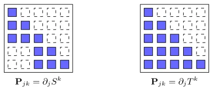
Several remarks are in order. First, we emphasize the fact that Theorem 3 characterizes sparsity patterns using only an I-map for νπ, without requiring any actual computation of the transports. One only needs to perform simple graph operations on G to build the sequence of graphs (Gk_{). See Figure 2 for an illustration of this procedure, with the} corre-sponding sparsity patterns in Figure 3. We refer to (Gk_{) as the} _marginal _{graphs. In fact,} the sequence (Gk) is precisely the set of intermediate graphs produced by the variable elim-ination algorithm (Koller and Friedman, 2009, Ch. 9), when marginalizing with elimelim-ination ordering (n, n−1, . . . ,1). This should not be surprising as the KR rearrangement is essen-tially a sequence of ordered marginalizations (Villani, 2008). The hypothesis that νη is a product measure is important for the theorem to hold. If we pick a reference measure with an arbitrary Markov structure, there need not exist a sparse transport map couplingνη and νπ, even if νπ has a sparse I-map. The role of a reference measure is somewhat peculiar to the world of couplings and is usually not addressed in classical treatments of graphical models. Nonetheless, this assumption on νη is not restrictive in the present framework,

(12)

since the reference distribution is considered a degree of freedom of the problem. Theorem 3 gives sufficient but not necessary conditions on (νη,νπ) for the existence of a sparse map. And it could not be otherwise: if νη = νπ then the identity map—the sparsest possible map—would be a valid coupling.

We also note that Theorem 3 does not provide the exact sparsity patterns of the trian-gular transport maps; instead, (12) and (13) provide subsets of I_T andI_S. In other words, the actual transport maps might be sparser than predicted by the sets bI_S and bI_T—but,

crucially, they cannot be less sparse. Thus, we can think of Theorem 3 as providingbounds on the sparsity of triangular transports. An important fact is that, without additional in-formation on νπ, these bounds are sharp. That is, we can always find a pair of measures (νη,νπ) satisfying the hypotheses of Theorem 3 and such that the predicted and actual sparsity patterns coincide, i.e.,bI_T =I_T orbI_S =I_S.

Part 3 of Theorem 3 shows that the predicted sparsity pattern of the inverse KR rear-rangement is always larger than or equal to that of the direct transport, i.e.,bI_T ⊂bIS. This

does not mean that for every pair of measures (νη,νπ), the inverse triangular transport is always at least as sparse as the direct transport; in fact, it is possible to provide simple counterexamples. However, this result does imply that if we are only given an I-map forνπ, then parameterizing candidate inverse triangular transports allows the imposition of more sparsity constraints than parameterizing candidate direct transports. In general, sparser transports are easier to represent. See Figure 4 (right) for a nontrivial example of sparsity patterns for a stochastic volatility model.

Indeed, (14) hints at a typical trend: inverse transport maps tend to be sparser (in many practical cases,much sparser) than their direct counterparts. Intuitively, the sparsity of a direct transport is associated with marginal independence in Z, whereas the inverse transport inherits sparsity from the conditional independence structure ofZ. The latter is a weaker condition than mutual independence; for instance, the correlation length of a process modeled by a Markov random field may be much larger than the typical neighborhood size (Rue and Held, 2005). Thus, given a sparse I-map for the target measure, it can be computationally advantageous to characterize an inverse transport rather than a direct one, because the inverse transport can inherit a larger sparsity pattern. Given an inverse triangular transport S, we can then easily evaluate the direct transport T = S−1 at any point x ∈ Rn by inverting S pointwise, as described in Section 3. There is no need to

have an explicit representation of the direct transport as long as it can be implicitly defined through its inverse.

5.2. Connection to Gaussian Markov Random Fields

The reader familiar with Gaussian Markov random fields (GMRFs), might see links between the preceding results and widespread approaches to the modeling of Gaussian fields. In this section, we clarify the extent of these connections.

(13)

interac-3

2 5

1 4

G5

3

2 5

1 4

G4

3

2 5

1 4

G3

5

2 4

1 3

G2

Figure 2: Sequence of graphs (Gk_{) described in Theorem 3 for a target measure in}_M+₍

R5)

with I-map illustrated by the leftmost graph, G5. Notice that to generate the graphG2, we remove node 3 fromG3 and turn its neighborhood into a clique by adding the edge (1,2).

Pjk=∂jSk Pjk=∂jTk

Figure 3: Sparsity patterns predicted by Theorem 3 for the target measure analyzed in Figure 2. We represent the sparsity patterns using a symbolic matrix notation: the (j, k)-th entry of the matrix isnot colored if the kth component of the map (S orT) does not depend on thejth input variable, or, equivalently, if (j, k)∈bI_S

(resp. bI_T) (12). (Since we are considering lower triangular transports, all entries

j > k are uncolored. Note also that Sk and Tk are always functions of their kth input by strict monotonicity of the map.) The predicted sparsity pattern for the direct transport in this example isbI_T =∅.

(14)

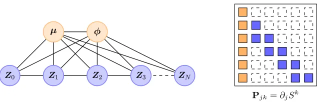
Z0 Z1 Z2 Z3 ZN

µ φ

Pjk=∂jSk

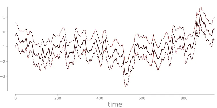
Figure 4: (left) Markov network for a stochastic volatility model (Kim et al., 1998). Blue nodes represent the discrete-time latent log-volatility process (Zk)Nk=0, which obeys a simple autoregressive model with hyperparametersµ,φ. The graph above is a minimal I-map for the posterior density described in Section 8,πµ,φ,Z0:N|y0:N,

wherey0:N are some (fixed) observations. (right) The predicted sparsity pattern

b

IS (only the top 6×6 block is shown) for the inverse transport corresponding to the model on the left: the first column/row of the matrix refer jointly to all of the hyperparameters. Each component Sk of the inverse transport can de-pend at most on four input variables, namely µ,φ,Zk−1,Zk, regardless of the overall dimension N of the problem. In order to apply the results of Theorem 3, we must select an ordering of the input variables; here, we used the ordering (µ,φ,Z0, . . . ,ZN). Optimal orderings are further discussed in Section 5.3.

Now the connection with Section 5.1 is clear: L> is an inverse triangular transport,6 while L−> is a direct one. Moreover, solving a triangular linear system is just a par-ticular instance of inverting a nonlinear triangular function by performing a sequence of one-dimensional root-findings. Thus the developments of the previous section, which con-sider arbitrarynonlinear maps, are a natural generalization—to thenon-Gaussiancase—of modeling and sampling techniques for high-dimensional GMRFs (Rue and Held, 2005).

5.3. Ordering of Triangular Maps

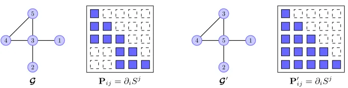
The results of Theorem 3 suggest that the sparsity of a triangular transport map depends on the ordering of the input variables. See Figure 5 for a simple illustration. Indeed, the triangular transport itself depends anisotropically on the input variables and requires the definition of a proper ordering. A natural approach is then to seek the ordering that promotes thesparsest transport map possible.

Consider a pair of measures (νη,νπ) that satisfies the hypotheses of Theorem 3. We associate an ordering of the input variables with a permutationσ onNn={1, . . . , n}, and define the reordered target measure ν_πσ as the pushforward of νπ by the matrix Qσ that represents the permutationσ. In particular, (Qσ)ij = (eσ(i))j, whereei is theith standard basis vector on Rn. Moreover, ifG is an I-map forνπ, then we denote an I-map for νπσ by

(15)

Gσ_{. Notice that}_Gσ _{can be derived from}_G _{simply by relabeling its nodes according to the} permutation σ. Then we can cast a variational problem for thebest orderingσ∗ as:

σ∗ ∈arg maxσ |IS| (15)

s.t. S]νπσ =νη

σ∈P(Nn),

where S is the KR rearrangement that pushes forward the reordered target ν_πσ to νη and

P(Nn) is the set of permutations of Nn. The goal is to maximize the cardinality of the sparsity pattern of the inverse map, |IS|. We restrict our attention to the sparsity of the inverse transport, since we know from Section 5.1 that the direct transport tends to be dense, even for the most trivial Markov structures.

Ideally, we would like to determine a good ordering for the map before computing the actual transport, and to use the resulting information about the sparsity pattern to sim-plify the optimization problem for S. However, evaluating the objective function of (15) requires computing a different inverse transport for each permutation σ. One possible way to relax (15) is to replaceIS with the predicted sparsity patternbI_S introduced in (12). The

advantage of this approach is that the objective function of the relaxed problem can now be evaluated in closed form without computing any transport map, but rather by performing the simple sequence of graph operations onGσ described by Theorem 3. The caveat is that, in general,bI_S ⊂I_S, and thus maximizing|bI_S|amounts to seeking the tightest lower bound

on the sparsity pattern of the inverse transport. From the definition ofbI_S, it follows that

the best orderingσ∗ for therelaxed problem is one that introduces the fewest edges in the construction of the marginal graphs Gn_{, . . . ,}_G1_{, whenever} _Gn ₌ _Gσ∗_{. Thus, for a given} I-map G, we denote by F(σ;G) the fill-in produced by the ordering σ. That is, F(σ;G) is a set containing all the edges introduced in the construction of the marginal graphs (Gk) from Gσ_{. A computationally feasible relaxation of (15) is then given by:}

σ∗∈arg minσ |F(σ;G)| (16) s.t. σ ∈P(Nn).

(16) is a standard problem in graph theory; it arises in a variety of practical settings, including (most relatedly) finding the best elimination ordering for variable elimination in graphical models, or finding the permutation that minimizes the fill-in of the Cholesky factor of a positive definite matrix (George and Liu, 1989; Saad, 2003). From an algorithmic point of view, (16) is NP-complete (Yannakakis, 1981). This should not be surprising, as best– ordering problems are typically combinatorial in nature. Nevertheless, given its widespread applicability, a host of effective polynomial-time heuristics for (16) have been developed in past years (e.g., min-fill or weighted-min-fill, Koller and Friedman, 2009). Most importantly, (16) can be solved without ever touching the target measure (assuming, of course, that an I-mapG forνπ is known). As a result, the cost of finding a good ordering is often negligible compared to the cost of characterizing a nonlinear transport map via optimization.

6. Decomposability of Transport Maps

(16)

3

2 5

1 4

G Pij=∂iSj

5

2 3

1 4

G0

P0ij=∂iSj

Figure 5: Illustration of how a simple re-ordering of the input variables can change the (predicted) sparsity pattern of the inverse map. On the left,Grepresents an I-map for the target measure considered in Figure 2, with ordering (Z1, Z2, Z3, Z4, Z5), together with its sparsity patternbI_S. (See Figure 3 for details on the “matrix”

representation of sparsity patterns.) On the right, G0 is an I-map for the same target measure but with the ordering (Z1, Z2, Z5, Z4, Z3). The corresponding sparsity patternbI_S0 is now the empty set.

target measure. Though direct triangular transports also inherit some sparsity according to Theorem 3, they tend to be more dense.

This section shows that direct transports enjoy a different form of low-dimensional structure: decomposability. A decomposable transport map is a function that can be written as the composition of a finite number of low-dimensional maps, e.g., T =T1◦ · · · ◦T` for some integer`≥2. We use a very specific notion of low-dimensional map, as follows.

Definition 4 (Low-dimensional map with respect to a set) A mapM :Rn→Rnis

low-dimensional with respect to a nonempty set C ⊂ V '_N_n if

1. Mk(x) =xk for k∈ C

2. ∂jMk= 0 for j∈ C andk∈ V \ C.

The effective dimension ofM is the minimum cardinality|V \ C| over all setsC with respect to which M is low-dimensional.

In particular, up to a permutation of its components, we can rewriteM as:

M(x) =

MC¯(x_C¯) xC

,

where ¯C = V \ C denotes the complement of C in V, and where for any map M and set A = {a1, . . . , ak}, MA denotes the multivariate function x 7→ (Ma1(x), . . . , Mak(x)) obtained by stacking together the components of M with index in A. Thus M is the trivial embedding of a |C|-dimensional function into the identity map and has¯ effective dimension bounded by |C|¯ < n. It is not surprising, then, that a decomposable transport

(17)

The forthcoming analysis will considergeneral, and hence possibly non-triangular, trans-ports. Thus its scope is much broader than that of Section 5, where we only focused on the sparsity of triangular transports. Yet, we will show that triangular maps are the build-ing block of decomposable transports. The cornerstone of our analysis is Theorem 7, which characterizes the existence and structure of decomposable transports given only the Markov structure of the underlying target measure.

Our discussion will proceed in two stages: first, we show how to identify direct transports that decompose into two maps, i.e., T = T1 ◦T2, and then we explain how to apply this result recursively to obtain a general decomposition of the formT =T1◦ · · · ◦T`.

6.1. Preliminary Notions

Before addressing the decomposability of transport maps, we need to introduce two useful concepts: proper graph decompositions and generalized triangular functions. The decom-position of a graph is a standard notion (Lauritzen, 1996).

Definition 5 (Proper graph decomposition) Given a graphG = (V,E), a triple(A,S,B) of disjoint subsets of the vertex setV forms a proper decomposition ofGif (1)V =A∪S ∪B, (2) A andB are nonempty, (3) S separates A from B, and (4) S is a clique.

See Figure 6 (top left) for an example of a decomposition. Clearly, not every graph admits a proper decomposition; for instance, a fully connected graph does not have a separator set for nonemptyA and B. The idea we will pursue here is that graph decompositions lead to the existence of decomposable transports.

The notion of a generalized triangular function is perhaps less standard, but still rela-tively straightforward:

Definition 6 (Generalized triangular function) A function T : Rn → Rn is said to

be generalized triangular, or simply σ-triangular, if there exists a permutation σ of Nn such that the σ(k)th component of T depends only on the variables xσ(1), . . . , xσ(k), i.e.,

Tσ(k)₍_x_{) =}_Tσ(k)₍_x

σ(1), . . . , xσ(k)) for all x= (x1, . . . , xn) and for all k= 1, . . . , n.

We can think of a generalized triangular function as a map that is lower triangular up to a permutation. In particular, ifσ is the identity onNn, then aσ-triangular function is simply

a lower triangular map (see Section 3). To represent the permutationσ, we use the notation

σ({i1, . . . , ik}) ={σ(i1), . . . , σ(ik)} to denote an ordered set that collects the action of the permutation on the elements (ij). For example, ifT :R4 →R4 is a σ-triangular map with σ defined as σ(N4) ={1,4,2,3}, thenT will be of the form:

T(x) =



  

T1(x1)

T2₍_x

1, x4, x2)

T3(x1, x4, x2, x3)

T4(x1, x4)



  

for some collection (Tk). We regard each component Tσ(k) as a map Rk → R. We say

(18)

permutation σ of Nn, there exists a (νη-unique) monotone increasing σ-triangular map— which we call a σ-generalized KR rearrangement—that pushes forward νη toνπ. We give a constructive definition for a generalized KR rearrangement in Appendix A.

A key property of a σ-generalized KR rearrangement is that it allows different sparsity patterns to be engineered, depending onσ, in a map that is otherwise fully general—in the sense of being able to couple arbitrary measures inM+(Rn). This feature will be essential

to characterizing decomposable transport maps.

6.2. Decomposition and Graph Sparsification

We now characterize transports that decompose into a pair of low-dimensional maps, as described in the following theorem. We formulate the theorem for a generic target measure νi. Later we will apply the theorem recursively to a sequence (νi) of different targets.

Theorem 7 (Decomposition of transport maps) Let X ∼νη, Zi ∼νi, with νη,νi ∈ M+(Rn) and νη tensor product measure. Denote by η, πi a pair of nonvanishing densities for νη and νi, respectively, and assume that νi factorizes according to a graph Gi, which admits a proper decomposition (A,S,B). Then the following hold:

1. There exists a factorization of πi of the form

πi(z) = 1

c ψA∪S(zA∪S)ψS∪B(zS∪B), (17)

where ψA∪S is strictly positive and integrable, with c= R

ψA∪S.

2. For any factorization (17) and for any permutation σ of Nn with

σ(k)∈



 

 

S if k= 1, . . . ,|S|

A if k=|S|+ 1, . . . ,|A ∪ S| B otherwise,

(18)

there exists a nonempty family, Di, of decomposable transport maps T = Li ◦R parameterized by R∈R_i such that eachT ∈D_i pushes forward νη toνi and where:

(a) Li is a σ-generalized KR rearrangement that pushes forward νη to a measure with densityψA∪S(zA∪S)ηXB(zB)/c and is low-dimensional with respect to B.

(b) R_i is the set of maps Rn →Rn that are low-dimensional with respect to A and

that push forward νη to the pullback L]iνi ∈M+(Rn).

(c) If Zi+1 ∼L]_iνi, then Z_Ai+1 ⊥⊥Z_S∪Bi+1 andZ_Ai+1=XA in distribution.

(d) L]_iνi factorizes according to a graphGi+1 that can be derived from Gi as follows:

– Remove any edge from Gi that is incident to any node in A.

– For any maximal cliqueC ⊂ S ∪B with nonempty intersectionC ∩S, letjC be

the maximum integerj such that σ(j)∈ C ∩ S and turnC ∪ {σ(1), . . . , σ(jC)}

(19)

We first look at the theorem for i= 1 and let ν1 :=νπ and G1 :=G, where νπ denotes our usual target measure with I-mapG and where (A,S,B) denotes a decomposition ofG. Among the infinitely many transport maps from νη to νπ, Theorem 7 identifies a fam-ily of decomposable ones. The existence of these maps relies exclusively on the Markov structure of νπ: we just requireG to admit a (proper) decomposition.7

Each transport T ∈ D₁ pushes forward νη to νπ and is the composition of two low-dimensional maps, i.e., T = L1 ◦R for a fixed L1 defined in Theorem 7[Part 2a] and for some R ∈ R1. (We also write D1 := L1 ◦R1.8) The structure of these low-dimensional maps is quite interesting. Up to a reordering of their components, Theorem 7[Parts 2a and 2b] show thatL1 and R have an intuitive complementary form:

L1(x) =



 

LA₁(xS,xA)

LS₁(xS)

xB





, R(x) = 

 

xA

RS(xS,xB)

RB(xS,xB) 



. (19)

(If S = ∅, one can just remove LS₁ and RS from (19), and drop the dependence of the remaining components onxS.) In particular, L1 and R have effective dimensions bounded by|A ∪ S|and|S ∪ B|=|V \ A|, respectively (see Definition 4). Even though L1 and Rare low-dimensional maps, their composition is quite dense—in the sense of Section 5—and is in general nontriangular:

T(x) = (L1◦R)(x) =



 

LA₁(RS(xS,xB),xA)

LS₁(RS(xS,xB) )

RB(xS,xB)



 ,

and thus more difficult to represent and to work with. The key idea of decomposable transports is that they can be represented implicitly through the composition of their low-dimensional factors, similar to the way that direct transports can be represented implicitly through their sparse inverses (Section 5).

The sparsity patterns of L1 and R in (19) are needed for the theorem to hold. In particular,L1must be aσ-triangular function withσspecified by (18). Notice that (18) does not prescribe an exact permutation, but just a few constraints on a feasibleσ. Intuitively, these constraints say that L1 should be a function whose components with indices in S depend only on the variables inS (wheneverS 6=∅), and whose components with indices in Adepend only on the variables inA ∪ S. Thus, there is usually some freedom in the choice ofσ. Different permutations lead to different families of decomposable transports, and can induce different sparsity patterns in an I-map,G2, for L]₁νπ (Theorem 7[Part 2d]).

Part 2d of the theorem shows how to derive a possible I-map G2—not necessarily minimal—by performing a sequence of graph operations on G. There are two steps: one that does not depend onσ and one that does. Let us focus first on the former: the idea is to remove fromG any edge that is incident to any node inA, effectively disconnectingAfrom the rest of the graph. That is, ifZ2∼L]₁νπ, then, regardless ofσ,L1makesZA2 marginally

7. To obtain a proper decomposition ofG, one is free to add edges toGin order to turn the separator set

S into a clique (see Definition 5);νπstill factorizes according to any less sparse version ofG.

(20)

independent of Z_S∪B2 by acting locally on G. And not only that: L1 also ensures that the marginals of νη and L]₁νπ agree along A (see Theorem 7[Part 2c]). Thus we should really interpretL1 as the first step towards a progressive transport of νη toνπ. L1 is a local map: it can depend nontrivially only upon variables in xA∪S. Indeed, in the most general case,

|A ∪ S|is the minimum effective dimension of a low-dimensional map necessary to decouple A from the rest of the graph. The more edges incident to A, the higher-dimensional a transport is needed. This type ofgraph sparsificationrequires a peculiar “block triangular” structure forL1 as shown by (19): anyσ-triangular function withσ given by (18) achieves this special structure. The second step of Part 2d shows that if S 6=∅, then it might be necessary to add edges to the subgraph GS∪B, depending on σ.9 The relevant aspect ofσ

for this discussion is the definition of the permutation onto the first|S|integers. In general, there are|S|! different permutations that could induce different sparsity patterns inG2_{. We} shall see that permutations that add the fewest edges possible are of particular relevance.

6.3. Recursive Decompositions

The sparsity ofG2 is important because it affects the “complexity” of the maps inR₁: each

R ∈R1 pushes forward νη toL]₁νπ. More specifically, by the previous discussion, we can see how the role of each R ∈ R₁ is really only that of matching the marginals of νη and

L]₁νπ alongV \ A. A natural question then is whether we can break this matching step into simpler tasks, or, in the language of this section, whether R1 contains transports that are further decomposable. Intuitively, we are seeking a finer-grained representation for some of the transports in R1. The following lemma (for i= 1) provides a positive answer to this question as long as V \ A is not fully connected inG2. From now on, we denote (A,S,B) by (A₁,S₁,B₁), since we will be dealing with a sequence of different graph decompositions. Lemma 8 (Recursive decompositions) Let νη,νi,Gi be defined as in the assumptions of Theorem 7 for a proper decomposition(Ai,Si,Bi) of Gi, while let Gi+1 andDi =Li◦Ri be the resulting graph (Part 2d) and family of decomposable transports,10respectively. Then there are two possibilities:

1. S_i∪ B_i is not a clique in Gi+1_{. In this case, it is possible to identify a proper} de-composition (Ai+1,Si+1,Bi+1) of Gi+1 for some Ai+1 that is a strict superset of Ai by (possibly) adding edges to Gi+1 in order to turn Si+1 into a clique. Let Di+1 =

Li+1◦Ri+1 be defined as in Theorem 7 for the pair of measures νη,νi+1 :=L]_iνi and (A_i+1,S_i+1,B_i+1). Then the following hold:

(a) Ri ⊃Di+1 and Li◦Ri ⊃Li◦Li+1◦Ri+1.

(b) Li+1 is low-dimensional with respect to Ai∪ Bi+1 and has effective dimension bounded by |(Ai+1\ Ai)∪ Si+1|.

(c) Each R∈Ri+1 has effective dimension bounded by |V \ Ai+1|.

9. This is not always the case. For instance, ifS is a subset of every maximal clique ofG inS ∪ B that has nonempty intersection withS, then, by Theorem 7[Part 2d], no edges need to be added.

10. Whenever we do not specify a permutationσi or a factorization (17) in the definition ofLi, it means

(21)

2. S_i∪ B_i is a clique in Gi+1_{. In this case, the decomposition of Part 1 does not exist.}

Lemma 8[Part 1] shows that if S1 ∪ B1 is not fully connected in G2, then there exists a proper decomposition (A2,S2,B2) of G2 (obtained, possibly, by adding edges to G2 in V \ A₁) for whichA₂ is a strict superset ofA₁. One can then apply Theorem 7 for the pair νη,ν2=L]₁ν1 and the decomposition (A2,S2,B2). As a result, Part 1a of the lemma shows that R₁ contains a subset D₂ = L2◦R2 of decomposable transport maps where both L2 and each R ∈R2 are local transports on V \ A1, i.e., they are both low-dimensional with respect to A1. In particular, L2 is responsible for decoupling A2\ A1 from the rest of the graph and for matching the marginals of νη and L]2L

]

1νπ = (L1◦L2)]νπ along A2\ A1. The effective dimension ofL2 is bounded above by the size of the separator set S2 plus the number of nodes inA₂\ A₁ (Part 1b of the lemma). The effective dimension of eachR∈R₂

is bounded by the cardinality of V \ A2 and is, in the most general case, lower than that of the maps in R₁ (Part 1c). Moreover, by Part 1a, D₁ =L1 ◦R1 ⊃L1 ◦L2◦R2, which means that among the infinitely many decomposable transports that push forwardνη toνπ, there exists at least one that factorizes as the composition of three low-dimensional maps as opposed to two, i.e., T =L1◦L2◦R for someR∈R2.

If, on the other hand, S₁∪ B₁ is fully connected in G2_{, then by Lemma 8[Part 2] we} know that the decomposition of Part 1 does not exist. As a result, we cannot use Theorem 7 to prove the existence of more finely decomposable transports in R₁. In other words, if we want to match the marginals ofνη and L]1νπ alongV \ A1 =S1∪ B1, then we must do so in one shot, using a singletransport map.

The main idea, then, is to apply Lemma 8[Part 1], recursively, k times, where kis the first integer (possibly zero) for which S_k+1∪ B_k+1 is a clique in Gk+2_{. After} _k _iterations, the following inclusion must hold:

D₁ =L1◦R1 ⊃L1◦ · · · ◦Lk+1◦Rk+1, (20) which shows that there exists a decomposable transport,

T =L1◦ · · · ◦Lk+1◦R, (21) for some R∈R_k+1, that pushes forwardνη toνπ. (Note that we can apply Lemma 8[Part 1] only finitely many times since|V \ A_i+1|is an integer function strictly decreasing iniand bounded away from zero.) Each Li in (20) is aσi-triangular map for some permutation σi that satisfies (21), and is low-dimensional with respect to Ai−1∪ Bi, i.e., for i > 1 and up to a permutation of its components,

Li(x) =



   

xAi−1

LAi\Ai−1

i (xSi,xAi\Ai−1) LSi_i (xSi)

xBi



   

.

(22)

sets (A_i) are nested, i.e.,A₁ ⊂ · · · ⊂ A_k+1.) Figure 6 illustrates the mechanics underlying the recursive application of Lemma 8.

We emphasize that the existence and structure of (21) follow from simple graph opera-tions on G, and do not entail any actual computation with the target measureνπ. Notice also that even if each map in the decomposition (20) isσ-triangular, the resulting transport mapT need not be triangular at all. In other words, we obtain factorizations of general and possibly non-triangular transport maps in terms of low-dimensional generalized triangular functions. In this sense, we can regard triangular maps as a fundamental “building block” of a much larger class of transport maps.

Decomposable transports are clearly not unique. In particular, there are two factors that affect both the sparsity pattern and the number k of composed maps in the family

L1 ◦ · · · ◦ Lk+1 ◦Rk+1: the sequence of decompositions (Ai,Si,Bi) and the sequence of permutations (σi). Usually, there is a certain freedom in the choice of these parameters, and each configuration might lead to a different family of decomposable transports. Of course some families might be more desirable than others: ideally, we would like the low-dimensional maps in the composition to have the smallest effective dimension possible. Recall that by Lemma 8 the effective dimension of each Li can be bounded above by |(Ai \ Ai−1) ∪ Si| (with the convention A0 = ∅). Thus we should intuitively choose a decomposition (A_i,S_i,B_i) ofGi _{and a permutation} _σ

i forLi that minimize the cardinality of (Ai\ Ai−1)∪ Si, and that, at the same time, minimize the number of edges added from

Gi to Gi+1. In principle, we should also account for the dimensions of all future maps in the recursion. In the most general case, this graph theoretic question could be addressed using dynamic programming (Bertsekas, 1995). In practice, however, we will often consider graphs for which agoodsequence of decompositions and permutations is rather obvious (see Section 7). For instance, if the target distributionνπ factorizes according to a treeG, then it is immediate to show the existence of a decomposable transportT =T1◦ · · · ◦Tn−1 that pushes forwardνη toνπ and that factorizes as the composition ofn−1 low-dimensional maps (Ti)ni=1−1, each associated to an edge ofG: it suffices to consider a sequence of decompositions (Ai,Si,Bi) withA1 ⊂ A2 ⊂ · · ·, where, for a given rooted version of G,Ai\ Ai−1 consists of a single node ai with the largest depth in GV\Ai−1, and where Si contains the unique

parent of that node. Remarkably, each mapTi has effective dimension less than or equal to two, independent of n—the size of the tree.

(23)

6.4. Computation of Decomposable Transports

Given the existence and structure of a decomposable transport like (21), what to do with it? There are at least two possible ways of exploiting this type of information. First, one could solve a variational problem like (6) and enforce an explicit parameterization of the transport map as the composition T =L1◦ · · · ◦Lk+1◦R. In this scenario, one need only parameterize the low-dimensional maps (Li, R) and optimize, jointly, over their composition. The advantage of this approach is that it bypasses the parameterization of a single high-dimensional function, T, altogether. See the literature on normalizing flows (Rezende and Mohamed, 2015) for possible computational ideas in this direction.

An alternative—and perhaps more intriguing—possibility is to compute the maps (Li) sequentially by solving separate low-dimensional optimization problems—one for each map

Li. By Theorem 7[Part 2a] and Lemma 8, there exists a factorization (17) of πi—a density ofL]_i₋₁νi−1—for which Li is aσi-generalized KR rearrangement that pushes forwardνη to a measure with density proportional to ψAi∪SiηXB_i, where (Ai,Si,Bi) is a decomposition

of Gi _and _Gi _{is an I-map for} _ν

i. In generalψAi∪Si depends on Li−1, and so the maps (Li)

must be computed sequentially.11 _{In essence, decomposable transports break the inference} task into smaller and possibly easier steps.

Note that we could define Li with respect to any factorization (17) with ψAi∪Si

in-tegrable: these different factorizations would lead to a family of decomposable transports with the same low-dimensional structure and sparsity patterns (as predicted by Theorem 7). Thus, as long as we have access to a sequence of integrable factors (ψAi∪Si), we can

com-pute each map Li individually by solving a low-dimensional optimization problem. (See Appendix A for computational remarks on generalized triangular functions.) Intuitively, since by Lemma 8[Part 1b] Li is low-dimensional with respect to Ai−1∪ Bi, we really only need to optimize for a portion of the map, namely LC_i forC = (A_i\ A_i−1)∪ Si, which can be regarded effectively as a multivariate map on R|C|. In the same way, the map R can

be computed as any transport (possibly triangular) that pushes forward νη toL]_k+1νk+1. Theorem 7[Part 2b] tells us that once again we only need to optimize for a low-dimensional portion of the map, namely,RSk+1∪Bk+1_.

While it might be difficult to access a sequence of factorizations (17) for a general problem, there are important applications, such as Bayesian filtering, smoothing, and joint parameter/state estimation, where the sequential computation of the transports (Li, R) is always possible by construction. We discuss these applications in the next section.

7. Sequential Inference on State-Space Models: Variational Algorithms

In this section, we consider the problem of sequential Bayesian inference (or discrete-time data assimilation; Reich and Cotter, 2015) for continuous, nonlinear, and non-Gaussian state-space models.

Our goal is to specialize the theory developed in Section 6 to the solution of Bayesian fil-tering and smoothing problems. The key result of this section is a new variational algorithm

11. This is not always the case. For instance, given a rooted version ofG and a pair of consecutivedepths

(see the discussion at the end of Section 6.3), all the maps (Li) associated with edges connecting nodes

(24)

A

1

S

1

B

1

2 3

1 6

4

5

A

1

S

1

B

1

2 3

1 6

4

5

A

2

S

2

B

2

2 3

1 6

4

5

A

2

S

2

B

2

2 3

1 6

4

5

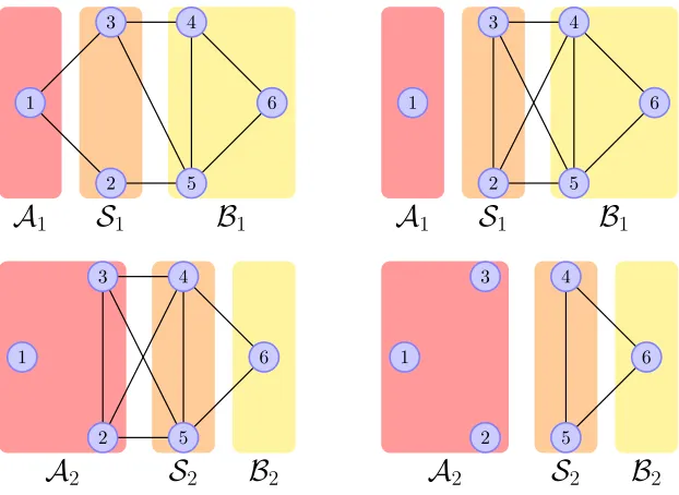
Figure 6: Sequence of graph decompositions associated with the recursive application of Lemma 8. On the(top left) there is an I-map, G1_{, for} _ν

π, with νπ ∈ M+(R6).

We first decompose this graph into (A1,S1,B1) as indicated, and apply Theorem 7 to the pair νη,νπ. To do so, we first need to add edge (2,3) to G1 in order to turn (A₁,S₁,B₁) into a proper decomposition of G1 _{with a fully connected} S1. The resulting graph, G1?, is now chordal (in fact, a triangulation of G1, Lauritzen, 1996), but still an I-map for νπ. The first map L1 is σ1-triangular withσ1(N6) ={2,3,1,4,5,6} and it is low-dimensional with respect to B1; The (top right)figure shows the I-map,G2_{, for}_L]

1νπ as given by Theorem 7[Part 2d]: as expected, A₁ is disconnected from S₁∪ B₁; moreover, a new maximal clique {2,3,4,5} appears in G2. This new clique is larger than any of the maximal cliques inG1

?, even thoughG1? is chordal. (Notice thatσ1 is not the permutation that adds the fewest edges possible inG2_{. An example of such “best” permutation} would beσ(N6) = {3,2,1,4,5,6}.) Though Theorem 7 guarantees the existence

of a low-dimensional map R ∈ R1 that pushes forward νη to L]1νπ, we instead proceed recursively by applying Lemma 8[Part 1] for a proper decomposition, (A₂,S₂,B₂), of G2_{, where}_A

2 is a strict superset of A1 (bottom left). The lemma shows thatR₁ ⊃L2◦R2for someσ2-triangular mapL2, which is low-dimensional with respect toA1∪B2, and where eachR∈R2 pushes forwardνη to (L1◦L2)]νπ. Can we apply Lemma 8 one more time to characterize decomposable transports inR₂? The answer is no, as the I-map for (L1◦L2)]νπ (bottom right) consists of a single clique inS2∪ B2. Nevertheless, eachR∈R2 is still low-dimensional with respect toA₂. Overall, we showed the existence of a transport mapT :R6→R6

(25)

for characterizing the full posterior distribution of the sequential inference problem—e.g., not just a few filtering or smoothing marginals—via recursive lag–1 smoothing with trans-port maps. The proposed algorithm builds a decomposable high-dimensional transtrans-port map in a single forward pass by solving a sequence of local low-dimensional problems, without resorting to any backward pass on the state space model (see Theorem 9). These results extend naturally to the case of joint parameter and state estimation (see Section 7.3 and Theorem 12). Pseudocode for the algorithm is given in Appendix C.

A state-space model consists of a pair of discrete-time stochastic processes (Zk,Yk)k≥0 indexed by the timek, where (Zk) is a latent Markov process of interest and where (Yk) is the observed process. We can think of eachYkas a noisy and perhaps indirect measurement ofZk. The Markov structure corresponding to the joint process (Zk,Yk) is shown in Figure 7. The generalization of the results of this section to the case of missing observations is straightforward and will not be addressed here.

We assume that we are given the transition densitiesπZk+1|Zkfor allk≥0, sometimes

re-ferred to as the “prior dynamic,” together with the marginal density of the initial conditions

πZ0. (For instance, the prior dynamic could stem from the discretization of a continuous

time stochastic differential equation; Oksendal, 2013.) We denote byπYk|Zk the likelihood

function, i.e., the density ofYkgiven Zk, and assume thatZkandYkare random variables taking values on Rn and Rd, respectively. Moreover, we denote by (yk)k≥0 a sequence of realizations of the observed process (Yk) that will define the posterior distribution over the unobserved (hidden) states of the model, and make the following regularity assumption in our theorems: πZ0:k−1,Y0:k−1 >0 for allk≥1. (The existence of underlying fully supported

measures will be left implicit throughout the section for notational convenience.)

Z0 Z1 Z2 Z3 ZN

Y0 Y1 Y2 Y3 YN

X0 X1 X2 X3 XN

Figure 7: (above) I-map for the joint process (Zk,Yk)k≥0 defining the state-space model. (below)I-map for the independent reference process (Xk)k≥0 used in Theorem 9.

7.1. Smoothing and Filtering: the Full Bayesian Solution

In typical applications of state-space modeling, the process (Yk) is only observed sequen-tially, and thus the goal of inference is to characterize—sequentially in time and via a recursive algorithm—the joint distribution of the current and past states given currently available measurements, i.e.,

(26)

for all k ≥ 0. That is, we wish to characterize π_Z_0:_k|y0:k based on our knowledge of the

posterior distribution at the previous timestep, πZ0:k−1|y0:k−1, and with an effort that is

constant over time. We regard (22) as the full Bayesian solution to the sequential inference problem (S¨arkk¨a, 2013).

Usually, the task of updating πZ0:k−1|y0:k−1 to yieldπZ0:k|y0:k becomes increasingly

chal-lenging over time due to the widening inference horizon, making characterization of the full Bayesian solution impractical for largek. Thus, two simplifications of the sequential infer-ence problem are frequently considered: filtering and smoothing (S¨arkk¨a, 2013). In filtering, we characterizeπZk|y0:k for all k≥0, while in smoothing we recursively update πZj|y0:k for

increasing k > j, where Zj is some past state of the unobserved process. Both filtering and smoothing deliver particular low-dimensional marginals of the full Bayesian solution to the inference problem, and hence are often considered good candidates for numerical approximation (Doucet and Johansen, 2009).

The following theorem shows that characterizing the full Bayesian solution to the se-quential inference problem via a decomposable transport map is essentially no harder than performing lag–1 smoothing, which, in turn, amounts to characterizing π_Z_k−₁_,_Z_k|y0:k for all

k ≥ 0 (an operation only slightly harder than regular filtering). This result relies on the recursive application of the decomposition theorem for couplings (Theorem 7) to the tree Markov structure of π_Z_0:_k|y0:k. In what follows, let (Xk)k≥0 be an independent (reference)

process with nonvanishing marginal densities (ηXk), with eachXktaking values onR

n_{. See} Figure 7 for the corresponding Markov network.

Theorem 9 (Decomposition theorem for state-space models) Let (Mi)i≥0 be a se-quence of (σi)-generalized KR rearrangements on Rn×Rn, which are of the form

Mi(xi,xi+1) =

"

M0_i(xi,xi+1)

M1_i(xi+1)

#

(23)

for some σi, M0_i :Rn×Rn→Rn, M1i :Rn→Rn, and that are defined by the recursion: – M0 pushes forward ηX0,X1 toπ

0 ₌

e

π0/c0, – M_i pushes forward ηXi,Xi+1 toπ

i₍_z

i,zi+1) =ηXi(zi)eπ