Task-Driven Common Representation Learning via Bridge Neural Network

The Thirty-Third AAAI Conference on Artificial Intelligence (AAAI-19)

Task-Driven Common

Representation Learning via Bridge Neural Network

Yao Xu,

Xueshuang Xiang,

Meiyu Huang

1_{Qian Xuesen Laboratory of Space Technology, China Academy of Space Technology, Beijing, 100190}

2_{School of Aerospace Science and Technology, Xidian University, Xian, 710071}

{xuyao, xiangxueshuang, huangmeiyu}@qxslab.cn

Abstract

This paper introduces a novel deep learning based method, named bridge neural network (BNN) to dig the potential rela-tionship between two given data sources task by task. The proposed approach employs two convolutional neural net-works that project the two data sources into a feature space to learn the desired common representation required by the specific task. The training objective with artificial negative samples is introduced with the ability of mini-batch train-ing and it’s asymptotically equivalent to maximiztrain-ing the total correlation of the two data sources, which is verified by the theoretical analysis. The experiments on the tasks, including pair matching, canonical correlation analysis, transfer learn-ing, and reconstruction demonstrate the state-of-the-art per-formance of BNN, which may provide new insights into the aspect of common representation learning.

Introduction

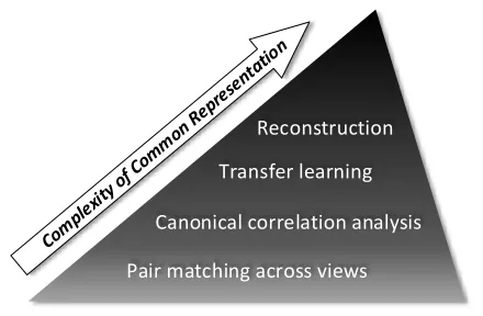
In the real world, a potential relationship always exists be-tween two sets of data, which can be either from multi-views of one data source, e.g., two voices of songs, audio and subti-tles of movies, or from two different data sources, e.g., faces of couples, objects with the same labels. One idea of min-ing the potential relationship of given data pairs is learnmin-ing a common representation of them, which has achieved lots of interests (Ngiam et al. 2011; Eisenschtat and Wolf 2017; Andrew et al. 2013; Chandar et al. 2016). These methods tried to build a universal model motivated by more than one task, including (i) pair matching across views, (ii) canoni-cal correlation analysis (CCA) (Hotelling 1936), (iii) trans-fer learning and (iv) reconstruction of a missing view. How-ever, different task imposes different complexity levels of common representations, as shown in Figure 1.

To clarify Figure 1, the complexity level of common rep-resentations for each task will be described briefly, from simple to complex. (i) For the task of pair matching across views, the common representations are just some poten-tial information which can build a connection between data pairs. This connection can be just a few similarities between pairs, which can be fairly simple. (ii) For the task of CCA, the common representations are the projections of two data

∗

Corresponding author.

Copyright c2019, Association for the Advancement of Artificial Intelligence (www.aaai.org). All rights reserved.

sources and it is supposed to maximize the linear correla-tion between them. CCA methods are always developed as a strategy to build common representations, which makes it an intermediate task rather than a final application objec-tive. (iii) For the task of transfer learning, the common repre-sentations need to be features which are useful for a certain learning objective, such as classification. The relationship of those features can be more complex than the linear correla-tion. (iv) Reconstruction of a missing view requires the com-mon representations to be an encoder, which should contain the information of the views as whole as possible.

Pair matching across views Canonical correlation analysis

Transfer learning Reconstruction

Figure 1: The complexity of common representations vary-ing from different tasks. A task on the top of the triangle is more complex than a bottom one.

Because of the diversity of different tasks, different tasks impose different levels of complexity of the common repre-sentations. Motivated by this understanding, we propose a novel deep learning based method, named bridge neural net-work (BNN) to learn common representations by mining the potential relationship of the specified data sources according to a given task, as shown in Figure 2. Given a task, we first construct the correlated data source, named positive sam-ples and build the negative samsam-ples according to the positive samples. Then both positive samples and negative samples are used to train a BNN to handle the given task.

de-Negative Sample

Positive Sample BNN Task

Figure 2: A framework of using Bridge Neural Network (BNN) to handle a task, e.g. as that shown in Figure 1.

termine whether two given data sources have a potential re-lationship, i.e. positive sample or not, i.e. negative sample. Thus, the problem of mining the potential relationship can be transferred to a binary classification problem by intro-ducing artificial negative samples. The main contributions of the proposed BNN in this paper are:

• First propose a task-driven framework to learn common representations by mining the potential relationship of given data pairs, which is specified task by task;

• A novel optimization problem, i.e. training objective us-ing artificial negative samples is introduced, and it’s asymptotically equivalent to maximization of the total correlation;

• BNN with lightweight convolution layers can be trained using Gradient Descent based optimization methods, making it more scalable for dealing with large high di-mensional data.

Related work

Canonical Correlation Analysis (CCA) (Hotelling 1936) is often used to build common representations. It is also a general procedure for investigating the relationships be-tween two sets of variables by computing a linear projec-tion for data pairs into a common space which can max-imize their linear correlation. It plays a significant role in many fields including biology and neurology (Hardoon et al. 2007), natural language processing (Dhillon, Foster, and Un-gar 2011), speech processing (Arora and Livescu 2013) and computer vision tasks, e.g., action recognition (Kim, Wong, and Cipolla 2007), linking text and image (Eisenschtat and Wolf 2017). CCA is also a basic method in multi-view learn-ing, see (Xu, Tao, and Xu 2013; Zhao et al. 2017) for details. However, traditional CCA method (Hotelling 1936) and its derivatives, such as regularized CCA (Vinod 1976), Nonparametric Canonical Correlation Analysis (NCCA) (Michaeli, Wang, and Livescu 2016), Random-ized Canonical Correlation Analysis (RCCA) (Mineiro and Karampatziakis 2014) and Kernel Canonical Correlation Analysis (KCCA) (Akaho 2006; Hardoon, Szedmak, and Shawe-Taylor 2004; Bach and Jordan 2002; Melzer, Re-iter, and Bischof 2001), do not scale well with the size of the dataset and the representations. A number of re-searches were therefore proposed to overcome this draw-back. Deep Canonical Correlation Analysis (DCCA) (An-drew et al. 2013) and its improved versions in image

and text matching (Yan and Mikolajczyk 2015; Wang, Li, and Lazebnik 2016) are one of those which introduced deep learning method. Based on DCCA, later works such as Correlation Neural Network(CorrNet) (Chandar et al. 2016) and Deep Canonically Correlated Autoencoders (DC-CAE) (Wang et al. 2015), brought in Multimodal Autoen-coder (MAE) (Ngiam et al. 2011) to extend the task of recon-struction of views. The introducing of MAE also improves the performance of CCA because it aims to capture a more meaningful common representation by adding an optimiza-tion objective minimizing the distance between the original input and the decoded output of each view. Along this line, 2-Way Nets (2WayNet) (Eisenschtat and Wolf 2017) gave a different approach by replacing the optimization objective into the Euclidean loss. In summary, these methods achieved the state-of-the-art performance, but still have some prob-lems, such as the scalability, high inference time with fully connected layers and most of these methods were to build a universal model motivated by more than one task.

In order to fix these problems, this paper proposes bridge neural network (BNN) with lightweight convolution layers to learn common representations by mining the potential re-lationship of the specified data sources according to a given task. The most related work is DCCA (Andrew et al. 2013), 2WayNet (Eisenschtat and Wolf 2017) and Siamese Net-work (Chopra, Hadsell, and LeCun 2005), which is a sim-ilar approach of using two networks to learn the simsim-ilarity between two inputs. Differences between BNN and each of them will be described in next section.

Bridge Neural Network

This section contains a detailed description of our proposed model. It is termed as Bridge Neural Network (BNN) be-cause it acts as a bridge connecting two sets of variables by projecting them to a common feature subspace. Instead of telling the neural network to use CCA to investigate the rela-tionship between two sets of variables (Andrew et al. 2013), we try to tell it which pairs of views are relevant and which are not, hoping the network to find a rule to analyze the po-tential relationship of the given data sources. The goal of BNN is to learn a common representation by mining the po-tential relationship of the specified data sources according to a given computer vision task.

Data sources

As we discussed in Figure 1, different tasks impose different complexity levels of common representations. Given a task, we should first construct the data pairs, which can learn com-mon representations of the corresponding complexity level. For example, suppose we try to build a model to match items across views, we can set the data pairs as the sets of two data sources, denoted by {X1, X2} ⊂ Rn1 _×

Rn2_,X

1 = {xi

1}Ni=1,X2={x2i}Ni=1. And the i-th componentxi1∈X1,

xi

2 ∈X2match each other. Here we defineSp ={xi1, xi2} as the positive sample set andSn ={xi1, x

j

2}, i6=j as the negative sample set. For the matching task, since the i-th componentsxi

Left CNN

●●● ●●●

Right CNN

1

0

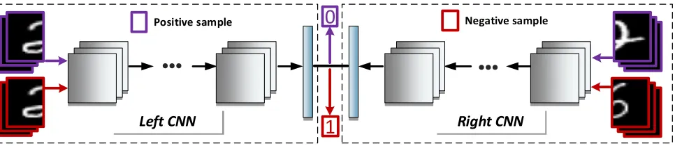
Figure 3: A schematic of bridge neural network, which employs two convolutional neural networks that project two given data sources into a common feature space. The Euclidean loss of the two output layers is supposed to close to0or1for positive samples or negative samples respectively. For the task of reconstruction of a missing view, transposed convolution networks should be introduced to make the common representation an encoder, see Figure 5.

not match the j-th componentxj₂ ∈X2,i 6=j. Actually, in practice, we may have two componentsxi

1, x

j

1 ∈ X1very close to each other. Ifxi

1matchesxi2andx

j

1matchesx

j

2, we may also havexi

1matchesx

j

2. Thus in the training process, the negative samples used to train BNN model are randomly selected fromSn, where we also take account the situation

that the size ofSnisN(N−1), that is almost square of the

size of positive sample. The details of constructing data pairs according to different computer vision task can be found in the Experiments.

Architecture

Our proposed network architecture is illustrated in Figure 3, which contains two convolutional neural networks: left CNN f1(·;θ1)and right CNNf2(·;θ2)with weights(θ1, θ2). For given input data pairs(x1, x2), the two outputs of left CNN and right CNN aref1(x1;θ1)andf2(x2;θ2)respectively. Both CNNs contain k hidden layers {h1, h2, ..., hk} and

each layer of the firstk−1 layers, contains a convolution layer, batch normalization, followed by the activation func-tion ReLU. Thek-th layer is a linear projection of the out-put of hk−1, followed by the sigmoid activation function. The BNN output of given input data pairs(x1, x2)is the Eu-clidean distance of the two outputs of left CNN and right CNN, that is defined as

f(x1, x2;θ1, θ2) =

1

√

n||(f1(x1;θ1)−f2(x2;θ2))||, (1) wherenis the dimension of the output ofhk, i.e., the

com-mon representation. We use a predefined threshold param-eter γ ∈ (0,1) onf(x1, x2;θ1, θ2) to determine whether input data pairs(x1, x2)have a potential relationship or not. According to the definition of the positive sample setSp

and negative sample setSn, BNN is supposed to judge that

the data pair inSp is relevant and the data pair inSnis not

relevant. Thus the BNN outputf(x1, x2;θ1, θ2)is supposed to be close to0 if(x1, x2) ∈ Sp and1 if(x1, x2) ∈ Sn.

Then define the loss on positive sample set as lp(Sp;θ1, θ2) =

1

|Sp|

X

(x1,x2)∈Sp

(f(x1, x2;θ1, θ2)−0)2, (2)

and the loss on negative sample set as

ln(Sn;θ1, θ2) =

1

|Sn|

X

(x1,x2)∈Sn

(f(x1, x2;θ1, θ2)−1)2, (3)

where BNN can be seen as a binary classification problem. Thus the overall loss of BNN onSpandSnis

Lbnn(Sp, Sn;θ1, θ2) =

lp(Sp;θ1, θ2) +α·ln(Sn;θ1, θ2)

1 +α ,

(4)

whereαis a parameter to balance the weights of positive samples and negative samples. Then the goal of BNN is, givenSpandSn, to find weights(θ∗1, θ∗2)such that

(θ₁∗, θ₂∗) = argmin_θ

1,θ2l(Sp, Sn;θ1, θ2). (5)

Relation with DCCA. Here we present a discussion of the relation between BNN and DCCA (Andrew et al. 2013). Besides the slight difference of basic architecture, i.e. DCCA uses fully connected layers and BNN uses convolu-tional layers, the main difference between DCCA and BNN is the optimization objective function. Since the motivation of DCCA is from the goal of canonical correlation analysis, the objective of DCCA is to find(θ₁∗, θ₂∗)which make the output layers of left and right CNN maximally correlated, that is

(θ₁∗, θ₂∗) = argmax_θ1,θ2corr(f1(X1;θ1), f2(X2;θ2)), (6)

which just involves the positive samples Sp. As that

Theorem 1 For a group of weights (θ∗1, θ∗2) obtained by (5), if the overall loss of BNN on Sp and Sn has l(Sp, Sn;θ1∗, θ2∗) → 0, then the outputs of BNN has

corr(f1(X1;θ1∗), f2(X2;θ∗2))→nasN → ∞.

Proof.To make the comparison more clear, we use the sim-ilar notations as that in DCCA (Andrew et al. 2013). Let H1 ∈ Rn×N, H2 ∈ Rn×N be matrices whose columns

are the outputs produced by the left CNN and right CNN on X1 and X2 of size N with weights (θ1∗, θ2∗). That is

H1=f1(X1;θ∗1),H2=f2(X2;θ∗2). LetH¯1=H1−_N1H11 be the centered data matrix (resp.H¯2), and defineΣˆ12 =

1

N−1H¯1H¯20, andΣˆ11= _N−11H¯1H¯10+r1Ifor regularization constantr1(resp.Σˆ22). Herer1 >0is chosen to makeΣˆ11 positive definite. Then by the discussion of Section 2 in (An-drew et al. 2013), the correlation, i.e., the total correlation of the topncomponents ofH1 andH2is the sum of the top

nsingular values of matrix T = ˆΣ−₁₁1/2Σˆ12Σˆ− 1/2 22 , that is exactly the trace of matrixT:

corr(H1, H2) =||T||tr= tr(T0T)1/2. (7)

Now we come to prove this theorem. For a group of weights(θ₁∗, θ₂∗)obtained by (5), if the overall loss of BNN onSpandSnhasl(Sp, Sn;θ1∗, θ2∗)→0, by the definition in (4), we have

lp(Sp;θ1∗, θ2∗)→0, ln(Sn;θ∗1, θ∗2)→0,

combined with the definition in (2) and (3), we obtain

f(x1, x2;θ1∗, θ2∗)→0, ∀(x1, x2)∈Sp, f(x1, x2;θ∗1, θ

∗

2)→1, ∀(x1, x2)∈Sn.

By the definition of f(x1, x2;θ∗1, θ∗2) in (1) and H1 =

f1(X1;θ∗1),H2=f2(X2;θ2∗), the above equations indicate that for the columns ofH1,hi1,i= 1, ..., Nand the columns ofH2,hi2,i= 1, ..., N,

||hi₁−hi₂|| →0, ||hi₁−hj₂|| →√n, i6=j, (8)

where the first equation meansH1→H2, which yields

¯

H1→H¯2. (9)

Notice that the output of each CNN is followed with sigmoid activation, then each entry of vectorhi

1 or hi2 is in (0,1), which yields thel-th entry satisfies|hi

1(l)−hi2(l)| ∈(0,1). Combined with the second equation in (8), we obtain for l= 1, ..., n,

|hi₁(l)−h₂j(l)| →1, i6=j. (10)

And sincehi

1(l), h

j

2(l)∈(0,1), then we have eitherhi1(l)→

0orhi2(l)→0, which leads tohi1(l)h

j

2(l) = 0,l= 1, ..., n. This means the inner product of vector hi

1 and hi2 has hhi

1, h

j

2i → 0,i 6= j, leading toH20H1 → D, whereD =

diag(hh1

1, h12i,hh21, h22i, ...,hhN1, hN2i). SinceH1→H2, we havehhi₁, hi₂i → ||hi₁||2_{, which meansDis close to a} posi-tive diagonal matrix. By the definition of centered data ma-trixH¯1,H¯2and a simple calculation, asN → ∞, we have

¯

H20H¯1→D. (11)

In order to simplify the discussion, suppose we have N = Kn with K ∈ Z. Then we can redefine H¯i =

( ¯Hi,1,H¯i,2, ...,H¯i,K) withH¯i,j ∈ Rn×n, i = 1,2, j = 1, ..., K. Then the diagonal matrixDcan also be redefined toD = (D1, D2, ...DK)withDj ∈ Rn×n,j = 1, ..., K.

Then the equation (11) meansH¯₂0_,jH¯1,j →Dj. SinceDis

close to a positive diagonal matrix, combined with lemma that the left inverse of a square matrix is the right inverse, we have H¯1,jH¯20,j → Dj and H¯1,j → H¯2,j according

to (9), thus we obtain H¯2,jH¯10,j → Dj. Then we have

¯

H2H¯10 →Dˆ :=

PK

j=1Dj, combined with (9), we have

¯

H1H¯10, H¯2H¯20, H¯2H¯10 →D,ˆ (12)

which means that the matrices Σˆ11,Σˆ12,Σˆ22 are close to a same positive diagonal matrix, leading toT → I. Com-bined with the definition ofcorr(H1, H2)in (7), andH1=

f1(X1;θ∗1),H2=f2(X2;θ∗2), asN → ∞we have

corr(f1(X1;θ∗1), f2(X2;θ∗2))→n.

This ends the proof.

We should remark that the above proof can be just asymp-totically understood. Actually, since we always haven

N, it’s impossible to haveH₂0H1be equal to a diagonal ma-trix. Theorem 1 is proposed to show that the objective of BNN is asymptotically equivalent to maximizing the corre-lation of the outputs of two CNNs on input data pairs, i.e. two views as that named in DCCA. In conclusion, the bene-fits of using BNN than DCCA can be summarized as

• Both for 1D signals and 2D signals, DCCA uses fully connected layers, while BNN uses convolutional lay-ers, which makes BNN less computation cost. There are around106_{learnable parameters in DCCA model, while} only about105parameters exist in our model.

• DCCA uses L-BFGS based pre-training strategy for a stochastic method on mini-batch training, but with no the-oretical analysis to verify the effectiveness of the training strategy and more cost in searching the pre-trained model. BNN proposes a novel optimization ob-jective with asymptotic equivalence to the maximization of the total correlation, and the objective can be easily used to a stochastic optimization procedure that operates on mini-batch data points one at a time.

Actually, there is a potential relation of using L-BFGS based pre-training strategy on the architecture for DCCA. Since DCCA uses fully connected layers, the pre-training of the weights in each layer can be formulated to find a local mini-mum of the total squared error of a reconstructing problem, where the L-BFGS second-order optimization method can be used. Otherwise, if DCCA uses convolutional layers, it will be complicated to use L-BFGS, since L-BFGS is more suitable to optimize a matrix.

the common Euclidean regression optimization problems. In conclusion, the benefits of using BNN than 2WayNet can be summarized as

• Both for 1D signals and 2D signals, 2WayNet uses fully connected layers to make the signal able to be re-constructed (but no reconstruction results are found in 2WayNet), while BNN uses convolutional layers, which makes BNN gain performance benefits when dealing with high dimensional inputs, such as datasets of large size im-ages.

• 2WayNet gives the lower bound analysis of the total cor-relation on the Euclidean loss, but with no upper bound analysis. Instead of just using Euclidean loss, the artificial negative sample is introduced in BNN to make the ob-jective asymptotically equivalent to the total correlation, which can be seen as another technique to handle the Eu-clidean regression optimization problems.

Relation with Siamese Network. Siamese Network (Chopra, Hadsell, and LeCun 2005) is a classical neural net-work architecture, which learns the similarity between two inputs. It consists of two identical neural networks, each tak-ing one of the two inputs. The similarity between them is then calculated by feeding the last layers of the two net-works into a contrastive loss function. BNN has a similar positive/negative-sample based optimization objective with Siamese Network, however there are three fundamental dif-ferences between them.

• The main task of Siamese Network is pair matching prob-lem, while BNN focuses on common representation learn-ing which can be used in variety tasks.

• The loss function of Siamese Network is a summa-tion of product between label and a Euclidean-based pre-designed loss, while the loss function of BNN is a Euclidean-based binary classification loss.

• Siamese Network shares weights for right and left net-works, while BNN has two totally independent networks which enable it to solve multimodal problems naturally.

Training process

Once the BNN model, i.e.{h1, h2, ..., hk}of left CNN and

right CNN, is defined, we can use a stochastic optimization procedure, e.g. SGD with mini-batch to train the weights given the training samples. Here we train the left CNN and the right CNN alternately in a single iteration, i.e. one mini-batch. As that discussed before, the negative samples used are randomly selected fromSn according to a predefined

parameterξ, named NP ratio, which denotes the ratio of the size of the negative samples on that of positive samples. See Algorithm 1 for the details of the training process of BNN.

Actually, using randomly selected negative samples is a trade-off strategy. In the ideal condition, we hope using all negative samples in the training, which is impossible in prac-tice. We compared the performance of the proposed negative sample generating strategy and the ideal one (training with all negative samples) based on a small sub-dataset. The dif-ference between the results of them is negligible.

Algorithm 1Training process of BNN

1: Construct positive samplesSp={xi1, xi2};

2: Define balance parameterα, learning rateηand NP ratio ξ;

3: Randomly initialize weightsθ1, θ2;

4: forEach epochdo

5: Randomly construct negative samples: Sn={xi1, x

j

2}, i6=jwith sizeN ξ;

6: formini-batchS_pi ⊂Sp, Sni ⊂Sndo

7: Update left CNN with

θ1←θ1−η

∂lbnn(Sip,S i n;θ1,θ2)

∂θ1 ;

8: Update right CNN with

θ2←θ2−η

∂lbnn(Sip,Sin;θ1,θ2)

∂θ2 ;

9: end for 10: end for

Experiments

In this section, three experiments are presented, includ-ing pair matchinclud-ing test, Canonical Correlation Analysis and transfer learning across views. We perform our experiments based on two datasets commonly used in the recent literature for CCA test: MNIST (LeCun et al. 1998) half matching and X-Ray Microbeam Speech data (XRMB) (Westbury 1994). As for the model we use in our experiment, both the left and right networks have structures of 3 successive convolution layers with 10 filters (3×3filters for MNIST,1×3filters for XRMB) and batch normalization. Each output of the last convolution layers of the two networks connects to a fully connected layer, linearizing into an-dimensional vector.

Actually, CNN is an optional choice in BNN. However, the experiments demonstrate that using lightweight CNN is a better choice since it can achieve the similar performances as that of using full-connected layers (For MNIST dataset, the corresponding accuracy, precision, recall of pair match-ing and CCA result is 92.10, 84.61, 93.29, 49.23). Here we ignore the detailed discussion of comparison.

Data Description

MNIST half matching MNIST handwritten digits image dataset (LeCun et al. 1998) is commonly used for train-ing various image processtrain-ing systems. The database con-tains 60,000 training images and 10,000 testing images of

28×28pixels. In our experiments, each image is cut into two28×14pixel halves vertically. Two strategies are used to construct positive and negative samples: 1) For matching test and CCA examination, we only consider two halves of the same images as positive samples. 2) For transfer learning across views, all pairs of halves from the same digits (with the same labels) are set as positive samples.

sam-ples are used for training and 10,000 for testing. Simultane-ous acSimultane-oustic and articulatory recording pairs are considered as positive samples.

Pair Matching Across Two Views

Among the existing works mentioned before, this task has not been explicitly implemented. Here we will only show our own results. On the testing data, we generate 10,000 pos-itive pairs and 20,000 negative pairs. The output dimension nof both networks is set to 50 for MNIST dataset, 112 for XRMB dataset, and the judging thresholdγis set to 0.5. To make the results more detailed, we also show the precision, recall, and F1 score in addition to the accuracy measure-ment.

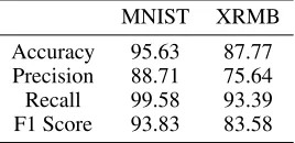
Table 1: Performance of pair matching test across two views learned by BNN on MNIST dataset (%).

MNIST XRMB

Accuracy 95.63 87.77

Precision 88.71 75.64

Recall 99.58 93.39

F1 Score 93.83 83.58

Table 1 suggests that BNN has a outstanding performance on pair matching test, especially the value of recall rate, which proves that BNN is able to learning exact features for accurately predict the relationship of two views as we expected.

(a) Top 100 False Positive Samples (b) Original Images

Figure 4: (a) Top 100 false positive samples. Samples out-lined in red are obviously negative for humans; (b) The orig-inal two images of those negative pairs outlined in (a).

Figure 4 (a) shows top 100 false positive samples on MNIST dataset. Most of those pairs are joined smoothly so that even humans will regard them as positive samples visu-ally. Though some of them are obviously negative samples, their original images are illegible (See Figure 4 (b)). In this case, the results can be considered as reasonable and accept-able.

Correlation between representations of two views

In this section, we will present the CCA result of BNN and compare it with the models we mentioned above. We fol-low Andrew’s Method (Andrew et al. 2013) calculating the total correlation captured in then=50 (MNIST) or n=112 (XRMB) dimensions of the common representations learned by the BNN. The structure of networks is the same as the one in the previous experiment. However, the testing data only contains positive samples, the same as all the experiments in the other works. The results are reported in Table 2. All CCA results of comparative models are stated in the literature of 2WayNet (Eisenschtat and Wolf 2017).

Table 2: Total correlation of the common representations learned by different models on MNIST and XRMB datasets.

Methods MNIST XRMB

CCA 28 16.9

DCCA 39.7 92.9

RCCA 44.5 104.5

DCCAE 25.34 41.47

CorrNet 48.07 95.01

2WayNet 49.15 110.18

BNN 49.32 110.65

Upper Bound 50 112

The reported values in Table 2 are the sum of the corre-lations captured in the 50 (MNIST) or 112 (XRMB) dimen-sions of the learned representations of the two views. The total correlations learned by BNN are closer to the max-imal value of 50 (MNIST) and 112 (XRMB), which are clearly better than the other models. Since the CCA results of 2WayNet are already very close to the maximum, any slight improvement can be considered significant.

Transfer Learning Across Views

In this section, all tests are implemented based on MNIST dataset. The experiment shows that the 50-dimension com-mon representation learned in BNN from the half views of the images can be trained to predict the digits of the other half views. Linear SVM classifier provided by Scikit-learn (Pedregosa et al. 2011) is used in our experiment and the common representaion data used to trian the SVM clas-sifier is inferenced by a well-trained and fixed BNN model. For each model list in Figure 3, we report 5-fold cross-validation accuracy on 10,000 images in the MNIST test dataset. Two sets of tests are reported: (i) training on the left views and testing on the right views, (ii) training on the right views and testing on the left views. All transfer learning re-sults of comparative models are stated in CorrNet (Chandar et al. 2016).

Table 3: Transfer learning (Left to Right, Right to Left) accu-racy using the representations learned using different models on the MNIST dataset.

Methods L. to R. R. to L.

CCA 65.73 65.44

DCCA 68.10 75.71

MAE 64.14 68.88

CorrNet 77.05 78.81

BNN 90.21 91.38

Single View 93.17 91.52

and 80.06 for left and right single views, the single view re-sults of BNN show that the learned common representations with only half digits are good enough for classification. In addition, the single view result is also the upper bound of our transfer learning performance. For BNN, the result of trans-fer learning accuracy is highly close to the accuracy of ideal single view case, indicating that the common representations captured by BNN gains excellent ability of transfer learn-ing. More importantly, it performs significantly better than all the other models as well. The high accuracy of transfer learning and single view on the representation indicates that the common representation found by BNN is much closer to the ideal common feature space for the classification task. Compared with the limited improvement on the task of to-tal correlation captured in Table 2, the huge improvement on transfer learning demonstrates the efficiency of using differ-ent positive samples task by task, since the training samples used in comparison methods are consistent across tasks.

Reconstruction Across Views

Firstly, we present the reconstruction architecture using BNN. Although MAE structure is unnecessary to learn common representations in our algorithm, view reconstruc-tion can be achieved by adding two transposed convolu-tion networks following the common representaconvolu-tion layers of BNN. The architecture is illustrated in Figure 5 which contains a standard bridge neural network and two trans-posed convolutional neural networks. For given input data pairs (x1, x2), the two outputs of the left CNN and right CNN are f1(x1;θ1) and f2(x2;θ2) respectively. For the given common representations (z1, z2) of the two views, the reconstruction of them are the outputs of the two trans-posed convolutional neural networks, which aref₁0(z1;θ10) andf₂0(z2;θ20)respectively.

To minimize the reconstruction error, new loss func-tions are introduced beside the loss of BNN (4). For self-reconstructions, we have the outputs of the two transposed convolutional neural networks asi= 1,2,

x0_{i sel}=f_i0(fi(xi;θi);θi0). (13)

Then we define the loss of self-reconstruction onSpas

lself(Sp;θ1, θ2, θ01, θ02) =

1

|Sp|

X

(x1,x2)∈Sp

(||x0_1sel−x1||+||x02sel−x2||). (14)

●●●

BNN

●●●

●●●

●●●

Left Transposed CNN

Right Transposed CNN

Figure 5: A schematic of bridge neural network with recon-struction structure, which employs a standard BNN (3) and two transposed convolutional neural networks.

For cross-reconstructions, we have two outputs as

x0_1cro=f₁0(f2(x2;θ2);θ10),

x0_2cro=f₂0(f1(x1;θ1);θ20).

(15)

Then we define the loss of cross-reconstruction onSpas

lcross(Sp;θ1, θ2, θ10, θ02) =

1

|Sp|

X

(x1,x2)∈Sp

(||x0_1cro−x1||+||x02cro−x2||). (16)

Thus the overall loss of BNN with reconstruction is

ltotal(Sp, Sn;θ1, θ2, θ10, θ02) =lbnn+lself +lcross. (17)

In the training process, i.e. Algorithm 1, we replace the loss lbnnwithltotaland update the weights in transposed

convo-lutional neural networksθ0

itogether withθi,i= 1,2.

(a)

(b)

(c)

(d)

(e)

Figure 6: Reconstruction results of BNN for MNIST. (a) Left view self-reconstruction; (b) Right view self-reconstruction; (c) Right to left cross-view reconstruction; (d) Left to right cross-view reconstruction; (e) Original images of two views.

Figure 6 shows the output images of self-reconstruction and cross-reconstruction both on left and right views of a few samples. The results are more clear and sharp both in self-reconstruction and cross-reconstruction compared with the visual results of CorrNet (Chandar et al. 2016). The visu-ally satisfying, which indicates that reconstruction can also be an optional function for Bridge Neural Network.

Conclusion

This paper proposes bridge neural network (BNN) with lightweight convolution layers to dig the potential relation-ship of two given data sources, that can be specified accord-ing to a computer vision task. The trainaccord-ing objective with the artificial negative samples is introduced and it’s asymptoti-cally equivalent to maximizing the total correlation of the two data sources in theory. The experiments on the tasks, in-cluding pair matching, canonical correlation analysis, trans-fer learning and reconstruction demonstrate the state-of-the-art performance of BNN.

Acknowledgements

This work was supported by the Innovation Foundation of Qian Xuesen Laboratory of Space Technology and the Na-tional Natural Science Foundation of China (61702520).

References

Akaho, S. 2006. A kernel method for canonical correlation analysis.arXiv preprint cs/0609071.

Andrew, G.; Arora, R.; Bilmes, J.; and Livescu, K. 2013. Deep canonical correlation analysis. InInternational Con-ference on Machine Learning, 1247–1255.

Arora, R., and Livescu, K. 2013. Multi-view cca-based acoustic features for phonetic recognition across speakers and domains. InAcoustics, Speech and Signal Processing (ICASSP), 2013 IEEE International Conference on, 7135– 7139. IEEE.

Bach, F. R., and Jordan, M. I. 2002. Kernel independent component analysis. Journal of machine learning research

3(Jul):1–48.

Chandar, S.; Khapra, M. M.; Larochelle, H.; and Ravindran, B. 2016. Correlational neural networks.Neural computation

28(2):257–285.

Chopra, S.; Hadsell, R.; and LeCun, Y. 2005. Learning a similarity metric discriminatively, with application to face verification. InComputer Vision and Pattern Recognition, 2005. CVPR 2005. IEEE Computer Society Conference on, volume 1, 539–546. IEEE.

Dhillon, P.; Foster, D. P.; and Ungar, L. H. 2011. Multi-view learning of word embeddings via cca. InAdvances in neural information processing systems, 199–207.

Eisenschtat, A., and Wolf, L. 2017. Linking image and text with 2-way nets.arXiv preprint.

Hardoon, D. R.; Mourao-Miranda, J.; Brammer, M.; and Shawe-Taylor, J. 2007. Unsupervised analysis of fmri data using kernel canonical correlation.NeuroImage37(4):1250– 1259.

Hardoon, D. R.; Szedmak, S.; and Shawe-Taylor, J. 2004. Canonical correlation analysis: An overview with applica-tion to learning methods.Neural computation16(12):2639– 2664.

Hotelling, H. 1936. Relations between two sets of variates.

Biometrika28(3/4):321–377.

Kim, T.-K.; Wong, S.-F.; and Cipolla, R. 2007. Tensor canonical correlation analysis for action classification. In

Computer Vision and Pattern Recognition, 2007. CVPR’07. IEEE Conference on, 1–8. IEEE.

LeCun, Y.; Bottou, L.; Bengio, Y.; and Haffner, P. 1998. Gradient-based learning applied to document recognition.

Proceedings of the IEEE86(11):2278–2324.

Melzer, T.; Reiter, M.; and Bischof, H. 2001. Nonlinear fea-ture extraction using generalized canonical correlation anal-ysis. InInternational Conference on Artificial Neural Net-works, 353–360. Springer.

Michaeli, T.; Wang, W.; and Livescu, K. 2016. Nonpara-metric canonical correlation analysis. InInternational Con-ference on Machine Learning, 1967–1976.

Mineiro, P., and Karampatziakis, N. 2014. A randomized algorithm for cca.arXiv preprint arXiv:1411.3409.

Ngiam, J.; Khosla, A.; Kim, M.; Nam, J.; Lee, H.; and Ng, A. Y. 2011. Multimodal deep learning. InProceedings of the 28th international conference on machine learning (ICML-11), 689–696.

Pedregosa, F.; Varoquaux, G.; Gramfort, A.; Michel, V.; Thirion, B.; Grisel, O.; Blondel, M.; Prettenhofer, P.; Weiss, R.; Dubourg, V.; et al. 2011. Scikit-learn: Machine learning in python. Journal of machine learning research

12(Oct):2825–2830.

Vinod, H. D. 1976. Canonical ridge and econometrics of joint production.Journal of econometrics4(2):147–166. Wang, W.; Arora, R.; Livescu, K.; and Bilmes, J. 2015. On deep multi-view representation learning. In International Conference on Machine Learning, 1083–1092.

Wang, L.; Li, Y.; and Lazebnik, S. 2016. Learning deep structure-preserving image-text embeddings. In Proceed-ings of the IEEE conference on computer vision and pattern recognition, 5005–5013.

Westbury, J. 1994. X-ray microbeam speech production database user’s handbook: Madison. WI: Waisman Center, University of Wisconsin.

Xu, C.; Tao, D.; and Xu, C. 2013. A survey on multi-view learning.Computer Science.

Yan, F., and Mikolajczyk, K. 2015. Deep correlation for matching images and text. In Computer Vision and Pat-tern Recognition (CVPR), 2015 IEEE Conference on, 3441– 3450. IEEE.