Gram–Schmidt Orthonormalization based
Projection Depth
Muthukrishnan R
1, Vadivel M
2, Ramkumar N
31Associate Professor, Department of Statistics, Bharathiar University, Coimbatore, Tamil Nadu, India 2, 3Research Scholar, Department of Statistics, Bharathiar University, Coimbatore, Tamil Nadu, India
Abstract—Gram-Schmidt Orthonormalization (GSO) Euclidean vectors based depth function is proposed to compute projection depth. The performance of GSO algorithm has been studied with exact and approximate algorithms, used in the associated estimator namelyStahel-Donoho (S-D) location and scatter estimators, for bivariate data.The efficiency of GSO algorithm is checked out by computing average misclassification error in discriminant analysis under real and stimulatingenvironment. The study concludesthat GSO algorithm based projection depth estimators performs well when compared with exact and approximate algorithms.
Keywords— Gram-Schmidt process, Projection depth, Robust Discriminant analysis.
I.
INTRODUCTION
Data depth is a function which quantifies the centrality of a point in a given data cloud. It is closely related to central regions or trimmed regions. It plays an important role in many notable fields of statistics,namely; data exploration, ordering, asymptotic distributions and robust estimation.Manydepth procedures have been developedin the past few decades, namely,half space depth [13], simplicial depth [7], regression depth [11] and projection depth [8],[18],[14].
Data depth has been used to compute multivariate measures of location and dispersion. In recent years data depth,based on projections has been increasingly studied and is mostly used in multivariate statistics. The essence of depth function in multivariate analyses is to measure the degree of centrality of a point relative to a data set. An analysis of multivariate statistical data is done by consideringeach univariate projection of the data. The main idea is, a central point is located in a multivariate data cloud only if it is located centrally in each univariate projection of this data cloud. The depth of a point in a multivariate data cloud is defined asthe minimum of the depths arising from the univariate projection of the data.
This paper is organized as follows. Section 2 describes the projection depth and associated estimator. Section 3 presents an abstract of various computational algorithms such as exact, fixed and random. The computational aspects of the proposed algorithm, namely, Gram-Schmidt Orthonormalization procedure is also furnished in the section. Section 4 examines the performance of the proposed GSO algorithm and critically compares the various algorithms of projection depth procedure through some examples. Section 5demonstrates the superiority of the GSO algorithm by applying it in the
discriminant analysis under real and simulation environment.
II. PROJECTION DEPTH AND ITS ASSOCIATED ESTIMATOR
[14]Established a projection-based depth function, which has the highest breakdown point among all the existing affine equivariant multivariate location estimators and associated medians. The projection depth is appeared very favorable to robust statistics when compared with the others depth notions.It is due to the reason that all the desirable properties of the general statistical depth function defined in [18], namely, affine invariance, maximality at center, monotonicity relative to deepest point, and vanishing at infinity are satisfied.Also, it can induce the favorable estimators, such as Stahel-Donohoestimator and depth weighted means for multivariate data [15], [16].[15]Introduced the concept of multidimensional trimming on projection depth. Exact computation of bivariate projection depth and Stahel-Donohoestimator,furthermore, with a proper choices of
,
are formulated and studied by [17].Furthercomputing issues of projection depth and its associated estimators has studied by [10]. The basic idea of computing, projection depth is summarized given below.Let µ (.) and σ (.)be univariate location and scale measures, respectively. Then the outlyingness of a point xR with respect to distribution functions F
of X in as[8], [14].
| ) F , x , u ( Q | sup ) F , x ( O
1 || u ||
(1)
where Q
x,F
uTx
F n
/
Fu and Fu is thedistribution of uTx. If uTx(Fu)
Fu 0 , and
u,x,F
0function robust choice of µ and σ is the median (Med) and the median absolute deviation (MAD). Let Fu be
the distribution furthermore, the projection depth and its associated estimator depend on the robust choice of (Med, MAD), Q(x, u, Xn) in (1) with respect to the unit vectors u in (1).
) X , x , u ( Q sup ) X , x ( O n 1 || u || n (2) where, ) X u ( MAD | ) X u ( Med x u | ) X , x , u (
Q T n
n T T
n
WhereuT denotes the projection of x onto the unit vector u anduTXn
uTX1,uTX2,...,uTXn
. Theprojection depth value of a given point x ε Rp with
respect to F can be defined as
)] F , X ( O 1 [ 1 ) F , X ( PD
The famous Stahel-Donoho location estimator [2], [12] i.e. the Projection Weighted Mean (PWM) and Projection Weighted Scatter (PWS) is given by
) dx ( F )) F , x ( PD ( W ) dx ( F )) F , x ( PD ( xW ) F ( PWM 1 1 (3) ) dx ( F )) F , x ( PD ( w ) dx ( F )) F , x ( PD ( w )) F ( PWM x ))( F ( PWM x ( ) F ( PWS 2 2 T (4)
WherePWM(F) and PWS(F) is the aforementioned Stahel-Donoho location and scatter estimators, w2(.)
denotes the weight function on [0, 1] based on projection depth outlying function (µ(F),σ(F)) as respectively. Note that the projection depth and its associated estimators awell defined, certain monotony conditions are required as follows
PD(x,F)
Fdx 0,wi
xiwiPDx,F Fdx ,i1,2.
With a finite sample Xn{X1,X2,...,Xn} from X and
Fn be the corresponding empirical distribution of F
based inXn.
III. GSO PROCEDURE OF COMPUTING PROJECTION DEPTH
In high dimensions, approximate algorithms include fixed and random direction procedures [17], [3] gives low efficiency. To enhance the efficiency and reduce the computational complexity, Gram-Schmidt orthogonal Euclidean vector based projections have been introduced to compute depth.
The fixed direction procedure uses fixed m directions which cut the upperhalfplane equally, and chooses the direction which can maximize (2). While random direction procedure randomly picks some m directions and chooses the optimal direction for computing the projection depth. The detailed computational steps are given by [3].An exact algorithm of computation of bivariate projection depth and the Stahel-Donoho estimator has been studied by [17]. Further, the simplified version of the computational procedure is given by [9].
In mathematics, particularly linear algebra and numerical analysis, the Gram-Schmidt process is a method for orthogonalnormalizationof vectors in an inner product space, most commonly the Euclidean space Rn equipped with the standard inner product. The Gram-Schmidt process takes a finite, linearly independent set S{v1,...,vk}for
k
n
and generates an orthogonal set S'{v1,...,vk}that spans the same k-dimensional subspace of Rn as S. The basic idea of Gram-Schmidt process is as follows: Let u1v1,and 1 k 1
j uj k
k
k v proj (v )
u (5)
where, ,
, , ) ( u u u v u v u proj
Here, u,v uTv, denotes the inner product of the
vectors u and v.Also, . u u e
k k
k The sequence u1,…,uk
is the orthogonal vectors, and the normalized vectors e1,…,ek form an orthonormal set. The computation of
the sequence u1,…,uk is known as Gram-Schmidt
orthogonalization, while the computation of the sequence e1,…,ek is known as Gram-Schmidt
orthonormalization as the vectors are normalized. When this process is implemented on the vectors 𝑢𝑘 are often not quite orthogonal, due to
rounding errors.The Gram-Schmidt process can be stabilized by a small modification. Instead of computing the vector 𝑢𝑘as in (5), it is computed as
) u ( proj u u , . . . , ) u ( proj u u , ) v ( proj v
u (k2)
k 1 k u ) 2 k ( k ) 1 k ( k ) 1 ( k 1 u ) 1 ( k ) 2 ( k k 1 u k ) 1 (
k each
step finds a vector (i) k
u orthogonal to (i1) k
u .Thus (i) k
u is also beingorthogonalized against any errors introduced in computation ofu(ki1).
IV. NUMERICAL ANALYSIS
This section presents some examples to examine the performance of a Matlab implementation of the proposed GSO algorithm alongwith exact and approximate algorithms.
A. Real Data
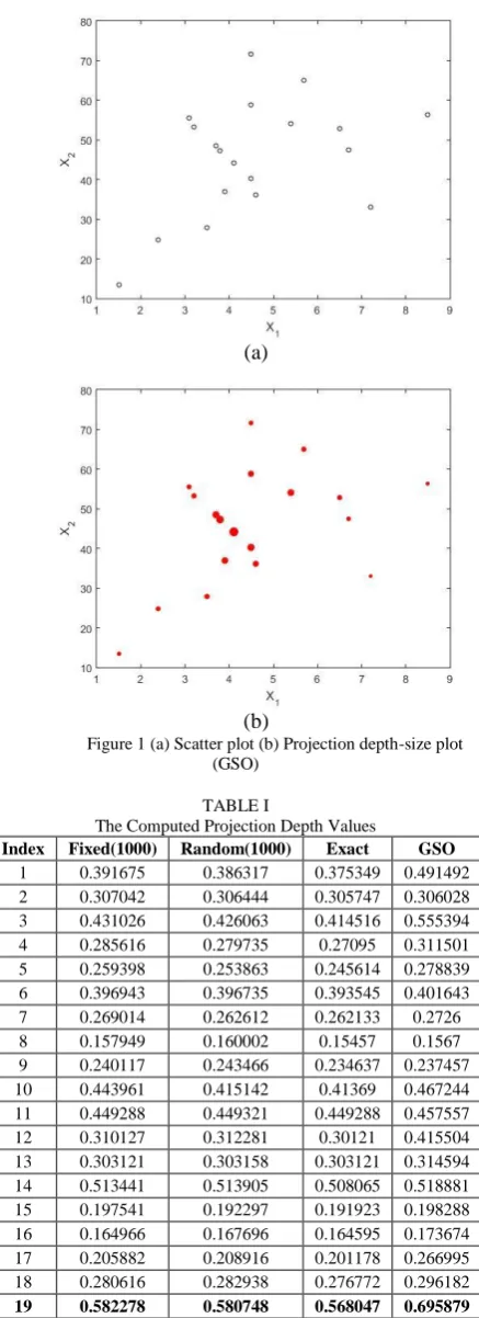
To illustrate the performance of projection depth, a real data example is presented. The data set is taken from [5] (Sweat data, Page 215). The data consists of 19 observations. The data describe 19 healthy females were measured with two variables sweat rate (X1) and sodium content (X2). The scatter
(a)
(b)
Figure 1 (a) Scatter plot (b) Projection depth-size plot (GSO)
TABLE I
The Computed Projection Depth Values
Index Fixed(1000) Random(1000) Exact GSO
1 0.391675 0.386317 0.375349 0.491492 2 0.307042 0.306444 0.305747 0.306028 3 0.431026 0.426063 0.414516 0.555394 4 0.285616 0.279735 0.27095 0.311501 5 0.259398 0.253863 0.245614 0.278839 6 0.396943 0.396735 0.393545 0.401643 7 0.269014 0.262612 0.262133 0.2726 8 0.157949 0.160002 0.15457 0.1567 9 0.240117 0.243466 0.234637 0.237457 10 0.443961 0.415142 0.41369 0.467244 11 0.449288 0.449321 0.449288 0.457557 12 0.310127 0.312281 0.30121 0.415504 13 0.303121 0.303158 0.303121 0.314594 14 0.513441 0.513905 0.508065 0.518881 15 0.197541 0.192297 0.191923 0.198288 16 0.164966 0.167696 0.164595 0.173674 17 0.205882 0.208916 0.201178 0.266995 18 0.280616 0.282938 0.276772 0.296182
19 0.582278 0.580748 0.568047 0.695879
It is noted that, all procedures represent the 19th observation as the location of a given data, since it has the largest depth value. Further comparing the depth value under various algorithms, the GSO gives the highest among them.
B. Simulation Results
A simulation study is performed to compare the efficiency of the proposed GSO procedure along with various notions of projection depth procedure. The data (n=25) are generated from a multivariate normal distribution, mean vector µ= (0,0) and the unit covariance matrix, =I2. The results are listed in table
2.
TABLE II
The Computed Projection Depth Values
S.N o
Fixed(100 0)
Random(10
00) Exact GSO
1
0.279751 0.279985
0.2797 51
0.2846 88 2
0.177699 0.177773
0.1776 99
0.1878 25 3
0.300351 0.300372
0.3002 42
0.3128 25 4
0.418745 0.419082
0.4187 45
0.4213 92 5
0.402708 0.402620
0.4025 44
0.4063 53 6 0.260813 0.261744 0.260813 0.262646
7
0.177237 0.177604
0.1771 37
0.1872 85 8
0.314549 0.315592
0.3145 49
0.3165 94 9
0.327815 0.327222
0.3264 25
0.3401 21 10
0.443497 0.443604
0.4434 97
0.4626 1 11
0.395648 0.395218
0.3948 40
0.4020 85 12
0.180137 0.180194
0.1800 76
0.1931 11 13
0.490847 0.491594
0.4908 47
0.4930 41 14
0.236695 0.236771
0.2366 22
0.2519 2 15
0.287932 0.288072
0.2879 32
0.2979 97 16
0.261341 0.262160
0.2613 41
0.2629 05
17
0.557417 0.558160
0.5574 17
0.5595 98
18
0.201091 0.201263
0.2010 91
0.2014 18 19
0.355026 0.355581
0.3550 26
0.3668 98 20 0.361799 0.361851 0.361799 0.369937
21
0.446930 0.446945
0.4469 30
0.4751 39 22
0.490172 0.490325
0.4901 72
0.5106 81 23
0.291422 0.291432
0.2914 22
0.3097 73 24
0.402583 0.402858
0.4025 83
0.4047 46 25
0.313248 0.313340
0.3132 48
0.3274 95
V. APPLICATION IN DISCRIMINANT ANALYSIS
The superiority of the GSO algorithm over the approximate and exact algorithms is studied by performing classification technique, namely discriminant analysis and compared the misclassification rate. [4] Developed the computational algorithm for fast and robust discriminant analysis, which is used for MATLAB implementation. The Stahel-Donoho estimator based projection depth approach is used for computing location and scatter values. Further, the analysis was performed simulated data with contamination.
A. Real Data
A real data set is taken from [6] (Page 584). The data consists of two different groups: π1 is
ridingmower owners and π2 is without
ridingmowers(non-owners) with each of sample 12. The owners or non-owners on the basis ofvariables, income (x1) and lot size (x2). The computed
group-wise misclassification and its averages are presented in Table 3.
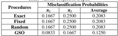
TABLE III
Computed Misclassification Probabilities under Various Projection Depths
Procedures πMisclassification Probabilities
1 π2 Average
Exact 0.1667 0.2500 0.2083
Fixed 0.1667 0.2500 0.2083
Random 0.1667 0.2500 0.2083
GSO 0.0833 0.1667 0.1250
It is observed that, the GSO algorithm gives very less average misclassification rate when compared with approximate and exact algorithms. That GSO procedure is misclassifies only 12%, but all other procedures misclassifies around 21% of the original data.
B. Simulation Result
To compare the GSO procedure with the approximate and exact procedure a simulation study is also performed with/without contamination. The data were generated from two different normal distributions (g=2, p=2) with varying sample sizes 50 and 100.The data were generated from thenormal distribution with covariance matrices ∑1=I2and ∑2=
1.5I2and means µ1= (1, 1) and µ2= (3, 3). The location
and scale contaminations are applied as described using the values of µ1= (-4, -4) and µ2= (-5, -5) along
with the covariance matrices ∑1 =3 I2and ∑2 = 2I2.The
various levels of contamination such as 0%,5%, 10%, 15% and 20% were considered in two cases also. The obtained results with the contamination are displayed in the table4.
TABLE IV
Computed Misclassification Probabilities under Various Contamination Levels
n1=n2=50
Error Exact Fixed Random GSO
0.00 0.0645 0.0645 0.0645 0.0645 0.05 0.0690 0.0690 0.0690 0.0690 0.10 0.0769 0.0769 0.0769 0.0718 0.15 0.0854 0.0854 0.0854 0.0769 0.20 0.0897 0.0897 0.0897 0.0824
n1=n2=100
0.00 0.0952 0.0952 0.0952 0.0952 0.05 0.0984 0.0984 0.0984 0.0984 0.10 0.1205 0.1205 0.1205 0.1193 0.15 0.1250 0.1250 0.1250 0.1236 0.20 0.1582 0.1582 0.1582 0.1429
It is noted that, when the contamination level increases misclassification probabilities is also increasing under all the procedures. On comparing the average probability of misclassification values in the above table, it is evident that the procedures GSO algorithm produces less when compared with exact and approximate algorithms. It is concluded that the GSO performs better than the exact and approximate algorithms. It shows that it is superior to the other algorithms under with/without contaminating data.
VI. CONCLUSION
This paper presents a novel idea of computing, projection depth. The computational aspect of the GSO algorithm is described. The performance of the GSO algorithm is discussed through numerical analysis. Further, the superiority of the GSO is demonstrated over the exact and approximate procedures by applying it in discriminant analysis under with/without contamination. It is concluded that, the performance of GSOprocedure is much better than approximate and exact algorithms. The study can be extended to higher dimensions. The new GSO procedure can be applied in almost all multivariate analysis and in turn it is very useful to research communities doing research in the field of data mining and computer vision.
ACKNOWLEDGEMENT
REFERENCES
[1] Ben Noble and James Daniel.: Applied Linear Algebra, 3rdedition. Prentice Hall, Englewood Cliffs, N.J., (1988). [2] Donoho, D. L., and Gasko, M.: Breakdown properties of
location estimates based on halfspace depth and projected outlyingness. The Annals of Statistics. 20, 1803–1827, (1992).
[3] Dyckerhoff, R,.:Data depthssatistiying the projection property. All emeinestatistischesArchiv, 88, 163-190, (2004).
[4] Hubert, M. and Van Driessen, K.: Fast and Robust Discriminant Analysis. Computaional Statistics and Data Analysis, 45,301,320, (2004).
[5] Johnson, R.A., and Wichern, D.W.: Applied multivariate analysis,3rd ed. Prentice Hall, Englewood Cliffs, New Jersey, (2007).
[6] Johnson, R.A., and Wichern, D.W.: Applied multivariate analysis, 9th ed. Prentice Hall, Englewood Cliffs, New
Jersey, (2009).
[7] Liu, R.Y.: On a notion of data depth based on random simplices. The Annals of Statistics, 18, 191-219, (1990). [8] Liu, R.Y.: Data depth and multivariate rank test. In: L1-
Statistical Analysis and Related Methods, 279-294. North-Holland, Amsterdam, (1992).
[9] Liu, X.H., Zuo, Y.J., Wang, Z.Z.: Exactly computing bivariate projection depth contours and median. Preprint, (2011).
[10] Liu, X., and Zuo, Y.: Computing projection depth and its associated estimators. Stat.Comput., 24, 51-63, (2014). [11] Rousseeuw, P.J., and Hubert, M.: Regression depth. Journal
of the American Statistical Association, 94, 388-433, (1999).
[12] Stahel, W.A.: Breakdown of covariance estimators. Research Report 31, 1029-1036, (1981).
[13] Tukey, J.W.: Mathematics and the picturing of data. In: Proceedings of the International Congress of Mathematicians, pp. 523-531. Canadian Mathematical Congress, Montreal, (1975).
[14] Zuo, Y. Projection-based depth functions and associated medians. The Annals of Statistics, 31, 1460-1490, (2003). [15] Zuo, Y.J.: Multidimensional trimming based on projection
depth. The Annals of Statistics, 34, 2211-2251, (2006). [16] Zuo, Y.J., Cui, H.J., He, X.M.: On the Stahel-Donoho
estimators and depth – weighted means for multivariate data. The Annals of Statistics, 32, 189-218, (2004). [17] Zuo, Y.J., and Lai, S.Y.: Exact computation of bivariate
projection depth and Stahel-Donoho estimator. Computational Statistics & Data Analysis, 55, 1173-1179, (2011).