A Two-Stage Penalized Least Squares Method for
Constructing Large Systems of Structural Equations
Chen Chen∗ [email protected]
Min Ren∗ [email protected]
Min Zhang [email protected]
Dabao Zhang [email protected]
Department of Statistics Purdue University
West Lafayette, IN 47907, USA
Editor:Xiaotong Shen
Abstract
We propose a two-stage penalized least squares method to build large systems of structural equations based on the instrumental variables view of the classical two-stage least squares method. We show that, with large numbers of endogenous and exogenous variables, the system can be constructed via consistent estimation of a set of conditional expectations at the first stage, and consistent selection of regulatory effects at the second stage. While the consistent estimation at the first stage can be obtained via the ridge regression, the adaptive lasso is employed at the second stage to achieve the consistent selection. This method is computationally fast and allows for parallel implementation. We demonstrate its effectiveness via simulation studies and real data analysis.
Keywords: graphical model, high-dimensional data, reciprocal graphical model, simul-taneous equation model, structural equation model
1. Introduction
We consider a linear system withpendogenous andqexogenous variables. With a sample of nobservations from this system, we denote the observed values of endogenous and exogenous variables byYn×p= (Y1,· · ·,Yp) andXn×q= (X1,· · · ,Xq), respectively. The interactions
among endogenous variables and the direct causal effects by exogenous variables can be described by a system of structural equations,
Y=YΓ+XΨ+, (1)
where the p×p matrix Γ has zero diagonal elements and contains regulatory effects, the q×pmatrixΨcontains causal effects, and is ann×p matrix of error terms. We assume that X and are independent of each other, and each component of is independently distributed as normal with zero mean while rows ofare identically distributed.
With gene expression levels and genotypic values as endogenous and exogenous variables, respectively, the model (1) has been used to represent a gene regulatory network with
∗. The first two authors contribute equally.
c
each equation modeling the regulatory genetic effects as well as the causal genomic effects from cis-eQTL (i.e., expression quantitative trait loci located within the regions of their target genes) on a given gene, see Xionget al. (2004), and Liuet al. (2008), among others. Genetical genomics experiments, which collect genome-wide gene expressions and genotypic values, have been widely undertaken to construct gene regulatory networks (Jansen and Nap, 2001; Schadt et al., 2003). However, fitting a system of structural equations in (1) to genetical genomics data for the purpose of revealing a whole-genome gene regulatory network is still hindered by lack of an effective statistical method which addresses issues brought by large numbers of endogenous and exogenous variables.
Several efforts have been made to construct the system (1) with genetical genomics data. Xionget al.(2004) proposed to use a genetic algorithm to search for genetic networks which minimize the Akaike Information Criterion (AIC; Akaike, 1974), and Liuet al.(2008) instead proposed to minimize the Bayesian Information Criterion (BIC; Schwartz, 1978) and its modification (Broman and Speed, 2002) for the optimal genetic networks. Both AIC and BIC are applicable to inferring networks for only a small number of endogenous variables. For a large system with many endogenous and exogenous variables, Cai et al.
(2013) proposed to maximize a penalized likelihood to construct a sparse system. However, it is computationally formidable to fit a large system based on the likelihood function of the complete model. Logsdon and Mezey (2010) instead proposed to apply the adaptive lasso (Zou, 2006) to fitting each structural equation separately, and then recover the network relying on additional assumption on unique exogenous variables. However, Caiet al.(2013) demonstrated its inferior performance via simulation studies, which is consistent with our conclusion.
Instead of the full information model specified in (1), we seek to establish the large system via constructing a large number of limited information models, each for one en-dogenous variable (Schmidt, 1976). For example, when the k-th endogenous variable is concerned, we focus on the k-th structural equation in (1) which models the regulatory effects of other endogenous variables and direct causal effects of exogenous variables, and ignore the system structures contained in other structural equations, leading to the following limited-information model,
Yk=Y−kγk+Xψk+k,
Y−k=Xπ−k+ξ−k.
(2)
HereY−krefers toYexcluding thek-th column,γkrefers to thek-th column ofΓexcluding
the diagonal zero, and ψk and k refer to the k-th columns ofΨ and respectively. The
second part of the model (2) is from the following reduced model by excluding the k-th reduced-form equation, withπ =Ψ(I−Γ)−1 and ξ=(I−Γ)−1,
Y=Xπ+ξ. (3)
In a classical low-dimensional setting, applying the ordinary least squares method to the first equation in (2) leads to underestimatedγk and ψk due to correlatedY−k and k.
Instead, the reduced-form equations in (2) are fitted to obtain least squares estimator ˆπ−k
of π−k, and least squares estimators of γk and ψk are further obtained by regressing Yk
(2SLS) method which can produce consistent estimates of the parameters when the system is identifiable. The 2SLS estimator was originally proposed by Theil (1953a,b, 1961) and, independently, Basmann (1957), and can be restated as the instrumental variables estimator (Reiersøl, 1941, 1945).
As in a typical genetical genomics experiment, we are interested in constructing a large system with the number of endogenous variables p possibly larger than the sample size n. Such a high-dimensional and small sample size data set makes it infeasible to directly apply the 2SLS method. Indeed,p≥nmay result in perfect fits of reduced-form equations at the first stage, which implies that we regress against the observed values of endogenous variables at the second stage and therefore obtain ordinary least squares estimates of the parameters. It is well known that such ordinary least squares estimates are inconsistent. Furthermore, constructing a large system demands, at the second stage, selecting regulatory endogenous variables among massive candidates, i.e., variable selection in fitting high-dimensional linear models.
In the setting of selecting instrumental variables (IVs) among a large number of candi-dates, L1 regularized least squares estimators have been recently proposed to replace the ordinary least squares estimator at the first stage of 2SLS (Belloni et al., 2012; Lin et al., 2015; Zhu, 2015). Belloni et al. (2012) applied lasso-based methods to select IVs and ob-tain consistent estimations at the first stage when the first stage is approximately sparse. For sparse instrumental variables models, Zhu (2015) proposed to replace with lasso-based methods at both stages of 2SLS and Lin et al. (2015) considered the representative L1 regularization methods and a class of concave regularization methods for both stages. All of these methods assume that each endogenous variable is only associated to a relatively small set of exogenous variables, i.e., each row of π in (3) only has a small set of nonzero components.
Here we consider to construct a general system of structural equations, which allows us to model nonrecursive or even cyclic relationships between endogenous variables. With the instrumental variables view of the two-stage approach, we observed that successful identification and consistent estimation of model parameters rely on consistent estimation of a set of conditional expectations which are optimal instruments. Therefore, establishing the system (1) in a high-dimensional setting is contingent on obtaining consistent estimation of these conditional expectations at the first stage, and effectively selecting and estimating of regulatory effects out of a large number of candidates at the second stage. Accordingly, we propose a two-stage penalized least squares (2SPLS) method to fit regularized linear models at each stage, withL2 regularized linear models at the first stage andL1 regularized linear models at the second stage.
the efficient computation makes it feasible to use the bootstrap method to evaluate the significance of regulatory effects.
The rest of this paper is organized as follows. First, we state an identifiable model in Section 2. Section 3 revisits the instrumental variables view on the classical 2SLS method, which motivates our development of the 2SPLS method in Section 4. We show in Section 5 the theoretical properties of the estimates from 2SPLS, with the proof included in the Appendix. Simulation studies are carried out in Section 6 to evaluate the performance of 2SPLS. An application to a real data set to infer a yeast gene regulatory network is presented in Section 7. We conclude this paper with a discussion in Section 8.
2. The Identifiable Model
We follow the practice of constructing system (1) in analyzing genetical genomics data (Logsdon and Mezey, 2010; Cai et al., 2013), and assume that each endogenous variable is affected by a unique set of exogenous variables, that is, the structural equation in (2) has known zero elements ofψk. Explicitly, we use Sk to denote the set of row indices of known nonzero elements inψk. Then we have known setsSk, k= 1,2,· · · , p, which dissect the set
{1,2,· · · , q}. We explicitly state this assumption in the below.
Assumption A.Sk 6=∅for k= 1,· · ·, p, butSj∩ Sk =∅ as long asj6=k.
The above assumption satisfies the rank condition (Schmidt, 1976), which is a sufficient condition for model identification. Since eachψk has a set of known zero components, from this point forward we ignore them and rewrite the structural equation in the model (2) as,
Yk=Y−kγk+XSkψSk+k, k ∼N(0, σ 2
kIn), (4)
where XSk refers to X including only columns indicated by Sk, and ψSk refers to ψk including only elements indicated bySk.
3. The Instrumental Variables View of the Two-Stage Least Squares Method
BecauseY−k andk are correlated, fitting merely the model (4) results in biased estimates
of γk and ψSk. However, the following two sets of variables are independent,
Z−k=E[Y−k|X] =Xπ−k,
εk=k+ξ−kγk.
Consequently, consistent estimates ofγkandψSk can be obtained by applying least squares method to the following model,
Yk =Z−kγk+XSkψSk+εk. (5)
Observing Y−kinstead ofZ−k =E[Y−k|X] naturally leads to application of the
instru-mental variables method (Reiersøl, 1941, 1945), that is, replacing Z−k = Xπ−k with its
estimate ˆZ−k=Xπˆ−k in fitting the linear model (5). When a
√
estimator of πj is obtained by fitting each equation in (3) for j = 1,· · · , p, the resultant
estimators of γk and ψSk are exactly the 2SLS estimators by Theil (1953a,b, 1961) and Basmann (1957).
Suppose that the matrix X satisfies the assumption in the below. It is easy to prove that, in a low-dimensional setting, we can obtain consistent estimators for the model (5) with any consistent estimate ofπ−k.
Assumption B. n−1XTX→C, whereCis a positive definite matrix.
Proposition 3.1 Suppose Assumptions A and B are satisfied for the system (1) with fixed
p n and q n. When there exists a consistent estimator πˆ−k of π−k, the ordinary
least squares estimators of (γk,ψSk) obtained by regressing Yk against (Xπˆ−k,XSk) are
also consistent.
The above instrumental variables view implies that the conditional expectation Z−k= E[Y−k|X] serves as the optimal instrument forY−k. Although, in a low-dimensional setting,
any consistent estimator ˆπ−k leads to the instrument ˆZ−k = Xπˆ−k, an efficient estimate
of π−k should be used to produce efficient estimates of γk and ψSk. In the following section, we build up on this view and construct the high-dimensional system (1) by first fitting high-dimensional linear models to consistently estimate the conditional expectations of endogenous variables given exogenous variables.
4. The Two-Stage Penalized Least Squares Method
To construct the limited-information model (2), we can obtain consistent estimates of the conditional expectations of endogenous variables given exogenous variables by fitting high-dimensional linear models, and then conduct a high-high-dimensional variable selection following our view on the model (5). Accordingly, we propose a two-stage penalized least squares (2SPLS) procedure to construct each model in (2) so as to establish the large system (1).
4.1 The Method
At the first stage, we use the ridge regression to fit each reduced-form equation in (3) to obtain consistent estimates of the conditional expectations of endogenous variables given exogenous variables, that is, for eachj= 1,2,· · · , p, we obtain the ridge regression estimator of πj by minimizing the following penalized sum of squares,
kYj−Xπjk22+τjkπjk22, (6)
where k · k2 is the L2 norm, and τj > 0 is a tuning parameter that controls the strength
of the penalty. The solution to the minimization problem is ˆπj = (XTX+τjI)−1XTYj,
which leads to a consistent estimate of Zj,
ˆ
Zj =PτjYj,
where Pτj =X(X
TX+τ
jI)−1XT. With a proper choice of τj, the ridge regression has a
At the second stage, we replace Z−k with ˆZ−k in model (5) to derive estimates of γk
andψSk, specifically, we minimize the following penalized error squares to obtain estimates of γk and ψSk,
1
2kYk−Zˆ−kγk−XSkψSkk 2
2+λkωTk|γk|, (7)
where|γk| denotes componentwise absolute value ofγk,ωk is a known weight vector, and λk>0 is a tuning parameter.
Minimizing for ψSk in (7) leads to
ˆ
ψSk = (XTSkXSk)
−1XT
Sk(Yk−Zˆ−kγk),
whereXSk is usually of low dimension, and the above least squares estimator ofψSk is easy to obtain.
Plugging ˆψS
k into (7), we can solve the following minimization problem to obtain an estimate ofγk,
ˆ
γk = arg min
γk
1
2(Yk−Zˆ−kγk)
TH
k(Yk−Zˆ−kγk) +λkωTk|γk|
, (8)
where Hk =I−XSk(X T SkXSk)
−1XT
Sk, this is equivalent to a variable selection problem in regressingHkYkagainst high-dimensionalHkZˆ−k. We will resort to adaptive lasso to select
nonzero components ofγkand estimate them. Specifically, picking up aδ >0 and obtaining ˜
γk as a√n-consistent estimate ofγk, we calculate the weight vector ωk with components
inversely proportional to components of |γ˜k|δ. The above minimization problem (8) is a
convex optimization problem which is computationally efficient.
4.2 Tuning Parameter Selection
In this method, we need to select tuning parameters at each stage. At the first stage, we propose to choose eachτj in (6) by the method of generalized cross-validation (GCV; Golub
et al., 1979), that is,
τj = arg min
τ >0Gj(τ) = arg minτ >0
(Yj −PτYj)T(Yj−PτYj)
(n−tr{Pτ})2
.
It is a rotation-invariant version of ordinary cross-validation, and leads to an approximately optimal estimate of the conditional expectationZj. At the second stage, the tuning
param-eter λk in (8) is obtained viaK-fold cross validation.
5. Theoretical Properties
5.1 The Number of Endogenous Variables is Fixed
ridge estimates ˆZ−k obtained from the first stage, we start with the theoretical properties
of ˆZ−k.
As mentioned previously, each τj in (6) is obtained by GCV. Interestingly, as stated by
Golubet al. (1979), such aτj is closely related to the one minimizing
Tj(τ) = (Zj−PτYj)T(Zj −PτYj).
We have the following result similar to Theorem 2 of Golubet al. (1979).
Theorem 5.1 Suppose that all components of πj are i.i.d. with mean zero and variance σπ2, then
arg min
τ >0E[E[Gj(τ)|πj]] = arg minτ >0E[E[Tj(τ)|πj]] =σ 2
ξj
σπ2,
where σ2ξ
j is the variance component of ξj in model (2).
This theorem implies that the GCV estimate ˆZj =PτjYj is approximately the optimal estimate of the conditional expectation Zj; furthermore, as the optimal tuning
parame-ter approximates a constant deparame-termined by the variance components ratio, we make the following assumption onτj.
Assumption C. τj/
√
n→0 asn→ ∞, forj= 1,· · · , p.
We then have the following properties on ˆZ−k.
Theorem 5.2 Fork= 1, . . . , p, letMk=πT−k(C−C•SkC −1
Sk,SkCSk•)π−k where eachCSrSc
is a submatrix ofCidentified with row indices inSrand column indices inSc(the dot implies
all rows or columns). Then, under Assumptions A, B, and C,
a. n−1ZˆT−kHkZˆ−k→p Mk, as n→ ∞;
b. n−1/2(Y
k−Zˆ−kγk)THkZˆ−k→dN(0, σk2Mk), asn→ ∞.
Since n−1ZT
−kHkZ−k → Mk, Theorem 5.2.a states that ˆZT−kHkZˆ−k is a good
approxi-mation toZT−kHkZ−k. On the other hand,Hk(Yk−Zˆ−kγk) is the error term in regressing
HkYk against HkZˆ−k, and Theorem 5.2.b implies that n−1(Yk−Zˆ−kγk)THkZˆ−k →d 0.
Thus ˆZ−k results in regression errors with good properties, i.e., the error effects on the
2SPLS estimators will vanish when the sample size gets sufficiently large.
In summary, the above theorem indicates that ˆZ−kbehaves the same way asZ−k
asymp-totically, which makes it reasonable to replace Z−k with ˆZ−k at the second stage. Denote
the j-th elements of γk and ˆγk as γkj and ˆγkj, respectively. Then, the properties of ˆZ−k
in Theorem 5.2, together with the oracle properties of the adaptive lasso, will lead to the following oracle properties of our proposed estimates.
Theorem 5.3 (Oracle Properties) LetAk={j:γkj 6= 0, j6=k}andAˆk={j: ˆγkj 6= 0, j 6=k}.
Further index both rows and columns of Mk with 1,· · · , k−1, k+ 1,· · · , p, and let Mk,Ak
be the submatrix of Mk identified with both row and column indices in Ak. Suppose that
λk/
√
n → 0 and λkn(δ−1)/2 → ∞. Then, under Assumptions A, B, and C, the estimates
a. Consistency in variable selection: limn→∞P( ˆAk=Ak) = 1;
b. Asymptotic normality: √n(ˆγk,Ak−γk,Ak)→dN(0, σ 2 kM
−1
k,Ak), asn→ ∞.
It is worth mentioning that Theorem 5.2 plays an essential role in establishing the oracle properties of 2SPLS. In fact, as long as the properties in Theorem 5.2 hold true for the first-stage estimates ofZ−k, the oracle properties can be expected from the adaptive lasso (Zou,
2006) at the second stage. On the other hand, we can also generalize the second-stage regularization to a wide class of regularization methods (Fan and Li, 2001; Huang et al., 2011; Zhang, 2010), the theoretical properties, of which, can still be inherited due to the results in Theorem 5.2.
5.2 The Number of Endogenous Variables is Divergent
In this section, we investigate the theoretical properties of 2SPLS with a divergentp. That is, per Assumption A, bothpandqmay grow with sample sizenat the the same order. The theoretical properties will be described by a prespecified sequence fn=o(n) but fn→ ∞.
We first update Assumptions B and C for the divergent p and q.
Assumption B0. Both p and q grow at the same order of o(n), i.e., p q = o(n). Furthermore, the singular values of I−Γ are positively bounded from below, and there exist positive constants c1 and c2 such that, for any vector δ with kδk2 = 1, c1 ≥n−1/2kXδk2≥c2.
Assumption C0. rnk ,τk2kπkk22/n=o(n).
We have the following properties on the ridge regression estimator of πk from the first
stage.
Theorem 5.4 Under Assumptions A, B0, and C0, for each ridge regression estimator πˆk,
there exist constants C1 and C2 such that, with probability at least 1−e−fn,
(a) kπˆk−πkk22 ≤C1(rnk∨q∨fn)/n;
(b) n−1kX( ˆπk−πk)k22≤C2(rnk∨q∨fn)/n.
Denote rmax = max1≤k≤prnk. Then the system-wise losses in both kπˆk−πkk22 and n−1kX( ˆπk−πk)k22 have upper bounds in the same order as (rmax∨q∨fn)/n, with
proba-bility at least 1−e−(fn−log(p)). Withp=o(n), we henceforth selectfn to dominate log(p),
i.e. fn−log(p)→ ∞, to guarantee the well-controlled losses over the whole system.
Denote Ak = {j:γkj = 06 , j 6=k}. Indexing all rows and columns with only j =
1,· · · , k−1, k+ 1,· · · , p, we define the restricted eigenvalue for a (p−1)×(p−1) matrix
Mas
φk(M) = min
n
n−1/2kMγk2kγAkk−12 :γAc
k
1 ≤3kγAkk1
o
.
We further define k · k∞ and k · k−∞ to be the maximum and minimum absolute values of the components of a vector, respectively. For a matrix,k · k∞is defined to be the maximum absolute row sum of the matrix.
We further make the following assumption on the tuning parameter λk of the adaptive
Assumption D. The adaptive tuning parameterλk is at the same order askωkk−1−∞kΓk1
kπk1pn(rmax∨q∨fn) logp.
We then have the consistency property of estimator ˆγk.
Theorem 5.5 (Estimation Consistency) Suppose that, for each node k, both inequalities
kωk,Akk∞kωk,Ackk −1
−∞ ≤ 1 and
p
(rmax∨q∨fn)/n+c1kπk1 ≤
q
c2 1kπk
2 1+φ20
64C2|Ak|
hold, and there exists a positive constant φ0 such that φk(HkXπ−k) ≥ φ0. Denote hn =
(kΓk21∧1)
h
(nqkπk21)∧(rmax∨q∨fn)
i
logp. Under Assumptions A, B0, C0, and D, there
exist constants C3 >0 and C4 >0 such that, with probability at least 1−e−C3hn+log(4pq)−
e−fn+log(p), each 2SPLS estimatorγˆk satisfies that 1. kγˆk−γkk1 ≤8C4
kωk,Akk∞kπk1kΓk
1
φ2
0kωkk−∞ |Ak|
q
(rmax∨q∨fn) logp
n ;
2. n−1
Hk
ˆ
Z−k(ˆγk−γk)
2 2≤
C2
4kωk,Akk∞2 kπk21kΓk 2
1
φ20kωkk2−∞
|Ak|(rmax∨q∨nfn) logp.
Note that the system-wide upper bounds, defined by replacing|Ak|with maxk|Ak|, can
also be achieved with probability at least 1−e−C3hn+log(4q)+2 log(p)−e−fn+2 log(p).
Let Wk = diag{ωk} and Vk = (vij)(p−1)×(p−1) , n1πT−kX TH
kXπ−k. Further denote Wk,Ak =diag{ωk,Ak},Wk,Ack =diag{ωk,Ack},Vk,21= (vij)i∈Ack,j∈Ak,Vk,11= (vij)i∈Ak,j∈Ak, and θk =
V
−1 k,11Wk,Ak
∞. We then have the following selection property.
Theorem 5.6 (Selection Consistency) Suppose that, for each node k, Vk,11 is invertible, andp(rmax∨q∨fn)/n+c1kπk1≤
q
c21kπk21+ min(φ20/64, ζ(4−ζ)−1kωkk−∞/θk)/(C2|Ak|).
Further assume that there exists a positive constant ζ ∈(0,1) such that min
j∈Ak
|γkj|> n2(2−λkθζk)
and
W
−1 k,Ac
kVk,21V −1 k,11Wk,Ak
∞<1−ζ. Under Assumptions A, B
0, C0, and D, there exists a
2SPLS estimatorˆγk satisfying that, with probability at least 1−e−C5hn+log(4pq)−e−fn+log(p)
for some constant C5 >0, Aˆk=Ak with Aˆk={j : ˆγkj 6= 0, j6=k}.
6. Simulation Studies
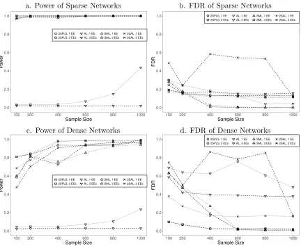
simulated to have the same number (either one or three) of nonzero exogenous effects (EEs) by the exogenous variables, with all effects equal to one. Each exogenous variable was simulated to take values 0, 1 and 2 with probabilities 0.25, 0.5 and 0.25, respectively, emulating genotypes of an F2 cross in a genetical genomics experiment. All error terms were independently simulated from N(0,0.12), and the sample size n varied from 100 to 1,000. For each network setup, we simulated 100 data sets and applied all four algorithms to calculate the power and false discovery rate (FDR).
For inferring acyclic networks, the power and FDR of the four different algorithms are plotted in Figure 1. 2SPLS has greater power than the other three algorithms to infer both sparse and dense acyclic networks when the sample size is small or moderate. When the sample size is large, 2SPLS, SML, and 2SAL are comparable for constructing both sparse and dense acyclic networks. In any case, AL has much lower power than other methods. Specifically, AL provides power as low as under 10% when the sample size is small, and its power is still under 50% even when the sample size increases to 1,000. On the other hand, 2SPLS provides power over 80% for small sample sizes, and over 90% for moderate to large sample sizes.
As shown in Figure 1, 2SPLS controls the FDR under 20% except for the case which has three available EEs with small sample sizes (n= 100). Although SML controls the FDR as low as under 5% for sparse acyclic networks when the sample sizes are large, it reports large FDRs when the sample sizes are small. For example, when the sample sizes are under 200, SML reports FDR over 40% for dense acyclic networks. In general, both 2SPLS and SML outperform AL and 2SAL in terms of FDR. Only in the case when inferring sparse acyclic networks with one available EE from data sets of moderate or large sample sizes, AL and 2SAL report FDR lower than 2SPLS.
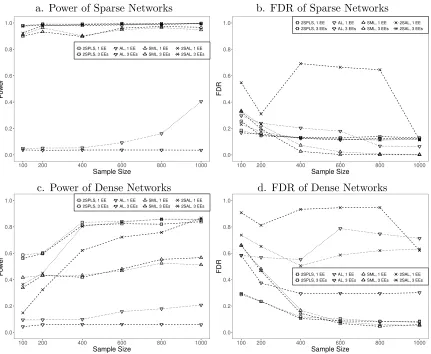
Plotted in Figure 2 are the power and FDR of the four different algorithms when inferring cyclic networks. Similar to the results on acyclic networks, 2SPLS has greater power than SML and AL across all sample sizes and has lower FDR when the sample size is small. 2SPLS has greater power than 2SAL in most scenarios and has much lower FDR than 2SAL except for the case when inferring sparse cyclic networks from data sets of large sample sizes. SML provides power competitive to 2SPLS for sparse cyclic networks, but its power is much lower than that of 2SPLS for dense cyclic networks. Similar to the case of acyclic networks, SML reports much higher FDR for inferring dense networks from data sets with small sample sizes though it reports small FDR when the sample sizes are large. 2SAL reports the highest FDR, especially for networks with three available EEs.
a. Power of Sparse Networks b. FDR of Sparse Networks
0.0 0.2 0.4 0.6 0.8 1.0
100 200 400 600 800 1000
Sample Size
P
o
w
er
2SPLS, 1 EE 2SPLS, 3 EEs
AL, 1 EE AL, 3 EEs
SML, 1 EE SML, 3 EEs
2SAL, 1 EE 2SAL, 3 EEs
0.0 0.2 0.4 0.6 0.8 1.0
100 200 400 600 800 1000
Sample Size
FDR
2SPLS, 1 EE 2SPLS, 3 EEs
AL, 1 EE AL, 3 EEs
SML, 1 EE SML, 3 EEs
2SAL, 1 EE 2SAL, 3 EEs
c. Power of Dense Networks d. FDR of Dense Networks
0.0 0.2 0.4 0.6 0.8 1.0
100 200 400 600 800 1000
Sample Size
P
o
w
er 2SPLS, 1 EE
2SPLS, 3 EEs AL, 1 EE AL, 3 EEs
SML, 1 EE SML, 3 EEs
2SAL, 1 EE 2SAL, 3 EEs
0.0 0.2 0.4 0.6 0.8 1.0
100 200 400 600 800 1000
Sample Size
FDR
2SPLS, 1 EE 2SPLS, 3 EEs
AL, 1 EE AL, 3 EEs
SML, 1 EE SML, 3 EEs
2SAL, 1 EE 2SAL, 3 EEs
Figure 1: Performance of 2SPLS, AL, SML, and 2SAL when identifying regulatory effects in acyclic networks with one EE or three EEs.
the first stage seems work well when each endogenous variable is associated to a small set of exogenous variables in (3), but may compromise the identification of regulatory effects at the second stage when the number of exogenous variables associated to an endogenous variable increases.
a. Power of Sparse Networks b. FDR of Sparse Networks
0.0 0.2 0.4 0.6 0.8 1.0
100 200 400 600 800 1000
Sample Size
P
o
w
er
2SPLS, 1 EE 2SPLS, 3 EEs
AL, 1 EE AL, 3 EEs
SML, 1 EE SML, 3 EEs
2SAL, 1 EE 2SAL, 3 EEs
0.0 0.2 0.4 0.6 0.8 1.0
100 200 400 600 800 1000
Sample Size
FDR
2SPLS, 1 EE 2SPLS, 3 EEs
AL, 1 EE AL, 3 EEs
SML, 1 EE SML, 3 EEs
2SAL, 1 EE 2SAL, 3 EEs
c. Power of Dense Networks d. FDR of Dense Networks
0.0 0.2 0.4 0.6 0.8 1.0
100 200 400 600 800 1000
Sample Size
P
o
w
er
2SPLS, 1 EE 2SPLS, 3 EEs
AL, 1 EE AL, 3 EEs
SML, 1 EE SML, 3 EEs
2SAL, 1 EE 2SAL, 3 EEs
0.0 0.2 0.4 0.6 0.8 1.0
100 200 400 600 800 1000
Sample Size
FDR 2SPLS, 1 EE
2SPLS, 3 EEs AL, 1 EE AL, 3 EEs
SML, 1 EE SML, 3 EEs
2SAL, 1 EE 2SAL, 3 EEs
Figure 2: Performance of 2SPLS, AL, SML, and 2SAL when identifying regulatory effects in cyclic networks with one EE or three EEs.
parameter at the first stage. SML is the slowest algorithm which generally takes more than 40 times longer than 2SPLS to infer different networks. In particular, SML is almost 200 times slower than 2SPLS when inferring acyclic sparse networks.
Acyclic Cyclic
Sparse Dense Sparse Dense
1 EE 3 EEs 1 EE 3 EEs 1 EE 3 EEs 1 EE 3 EEs
2SPLS 1303 1332 1127 1112 1297 1337 1125 1165
AL 405 652 404 637 443 659 430 781
SML 258875 195739 58509 43118 49393 58716 67949 68081
2SAL 3239 4726 3398 5357 3135 4681 3686 5651
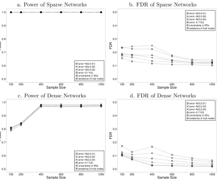
The robustness of 2SPLS was also evaluated from different aspects: (i) its robustness to different noise levels by doubling or even quadrupling the error variance; (ii) its robustness to non-normality of error terms by simulating errors sampled from a t-distribution, i.e., t(3); (iii) its robustness to uncertainty in the connections between exogenous and endogenous variables by simulating three exogenous effects for each endogenous variable (to emulate the genetical genomics experiment, the three exogenous variables are correlated with correlation coefficients at 0.8, and have effects at 1, 0.5, and -0.3, respectively) but including only one exogenous variable with the strongest estimated effects for each endogenous variable; (iv) its robustness to existence of hub nodes by simulating networks with six hub nodes having five regulatory effects on average while other endogenous variables having on average one regulatory effect for sparse networks, or three regulatory effects for dense networks. All networks include 300 endogenous variables, and the networks with errors following N(0,0.01) are the same as those shown in Figure 1. As shown in Figure 3, the 2SPLS method demonstrated robust power while the FDR was slightly affected when the error variance doubled. When the error variance quadrupled, a higher FDR was reported as expected. With errors from t(3), we observed similar power and slightly increased FDR of 2SPLS, which confirms the robustness of 2SPLS to non-normality. The uncertainty in the connections between exogenous and endogenous variables had almost no effect on the power of 2SPLS, and only slightly increased the FDR in constructing sparse networks. The existence of hub nodes rarely affected construction of dense networks, but decreased the FDR in constructing sparse networks. Overall, the performance of 2SPLS is remarkable in demonstrating robustness under a variety of realistic data structures.
7. Real Data Analysis
We analyzed a yeast data set with 112 segregants from a cross between two strains BY4716 and RM11-la (Brem and Kruglyak, 2005). A total of 5,727 genes were measured for their expression values, and 2,956 markers were genotyped. Each marker within a genetic region (including 1kb upstream and downstream regions) was evaluated for its association with the corresponding gene expression, yielding 722 genes with marginally significant cis-eQTL (p-value < 0.05). The set of cis-eQTL for each gene was filtered to control a pairwise correlation under 0.90, and then further filtered to keep up to three cis-eQTL which have the strongest association with the corresponding gene expression.
a. Power of Sparse Networks b. FDR of Sparse Networks
0.5 0.6 0.7 0.8 0.9 1.0
100 200 400 600 800 1000
Sample Size
P
o
w
er
error~N(0,0.01) error~N(0,0.02) error~N(0,0.04) error~0.1*t(3) uncertainty in EEs
existence of hub nodes 0.0 0.1 0.2 0.3 0.4 0.5
100 200 400 600 800 1000
Sample Size
FDR
error~N(0,0.01) error~N(0,0.02) error~N(0,0.04) error~0.1*t(3) uncertainty in EEs existence of hub nodes
c. Power of Dense Networks d. FDR of Dense Networks
0.5 0.6 0.7 0.8 0.9 1.0
100 200 400 600 800 1000
Sample Size
P
o
w
er
error~N(0,0.01) error~N(0,0.02) error~N(0,0.04) error~0.1*t(3) uncertainty in EEs
existence of hub nodes 0.0 0.1 0.2 0.3 0.4 0.5
100 200 400 600 800 1000
Sample Size
FDR
error~N(0,0.01) error~N(0,0.02) error~N(0,0.04) error~0.1*t(3) uncertainty in EEs existence of hub nodes
Figure 3: Performance of 2SPLS in robustness tests when identifying regulatory effects in acyclic networks with one EE.
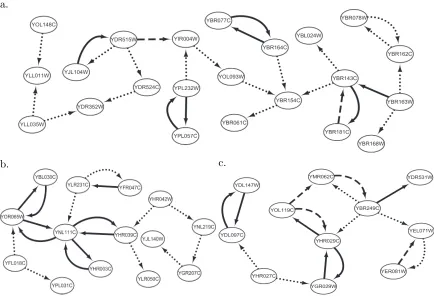
A gene-enrichment analysis with DAVID (Huang et al., 2009) showed that the three subnetworks are enriched in different gene clusters (controllingp-values from Fisher’s exact tests under 0.01). A total of six gene clusters are enriched with genes from the first sub-network, and four of them are related to either methylation or methyltransferase. Six of 22 genes in the first subnetwork are found in a gene cluster which is related to none-coding RNA processing. The second subnetwork is enriched in nine gene clusters. While three of the clusters are related to electron, one cluster includes half of the genes from the second subnetwork and is related to oxidation reduction. The third subnetwork is also enriched in nine different gene clusters, with seven clusters related to proteasome.
a.
b. c.
Figure 4: Three gene regulatory subnetworks in yeast (the dotted, dashed, and solid arrows implied that the corresponding regulations were constructed respectively from over 80%, 90%, and 95% of the bootstrap data sets).
8. Discussion
In a classical setting with small numbers of endogenous/exogenous variables, constructing a system of structural equations has been well studied since Haavelmo (1943, 1944). Anderson and Rubin (1949) first proposed to estimate the parameters of a single structural equation with the limited information maximum likelihood estimator. Later, Theil (1953a,b, 1961) and Basmann (1957) independently developed the 2SLS estimator, which is the simplest and most common estimation method for fitting a system of structural equations. However, genetical genomics experiments usually collect data in which both the number of endogenous variables and the number of exogenous variables can be very large, invalidating the clas-sical methods for building gene regulatory networks. It is noteworthy that, although each structural equation modeling gene regulation has few exogenous variables, the genome-wide gene regulatory network consists of a large number of structural equations and therefore has a large number of exogenous variables.
The instrumental variables view of 2SLS sheds light on the consistency of 2SLS estima-tors which is guaranteed by good estimation of the conditional expectations of endogenous variables given exogenous variables. For large systems, we proposed to estimate these con-ditional expectations via ridge regression coupled with GCV so as to address possible over-fitting issues brought by a large number of exogenous variables. We obtained approximately optimal estimation of these conditional expectations at the first stage. At the second stage, we could adopt results from high-dimensional variable selection, e.g., Fan and Li (2001), Zou (2006), Zhang (2010), and Huang et al. (2011), to consistently identify and further estimate the regulatory effects of the endogenous variables. As a high-dimensional exten-sion of the classical 2SLS method, the 2SPLS method is also computationally fast and easy to implement. As shown in constructing a genome-wide gene regulatory network of yeast, the high computational efficiency of 2SPLS allows us to employ the bootstrap method to calculate thep-values of the regulatory effects.
Our simulation studies show a seemingly counterintuitive result that our moment-based method 2SPLS provides higher power than the likelihood-based method SML, because the maximum likelihood method is usually the most efficient method, and dominates moment methods. However, as evidenced in Bollen (1996) and Kennedy (1985) (p.134), 2SLS can perform better than the maximum likelihood method in small samples. Furthermore, SML is not a pure likelihood method but rather a penalized likelihood method, and 2SPLS is not a pure moment method but rather a penalized moment method. Therefore, the theoretical advantage of likelihood methods over moment methods may not carry over to comparing penalized likelihood methods versus penalized moment methods. In fact, SML uses an L1 penalty to penalize nonzero regulatory effects, but 2SPLS employs an L2 penalty on the regression coefficients of the reduced models at the first stage and an L1 penalty on the regulatory effects at the second stage. We conjecture that the different choice of penalty terms may also distinguish the two different methods as shown in the advantage of the elastic net (Zou and Hastie, 2005) over lasso (Tibshirani, 1996).
polymor-phism from its cis-eQTL, which can be detected with classical eQTL mapping methods, e.g., Kendziorski et al.(2006), Gelfondet al.(2007), and Jia and Xu (2007). Trans-eQTL (i.e., eQTL outside the regions of their target genes) hold the key to our understanding of gene regulation because their indirect regulations are likely caused by interactions among genes. When the gene regulatory network is modeled with a system of structural equations, clas-sical eQTL mapping methods essentially identify both cis-eQTL and trans-eQTL involved in each reduced-form equation in the reduced model (3). Nonetheless, it is challenging, if not impossible, to recover a large system from the reduced model.
An alternative strategy to construct the whole system is to build undirected graphs first (Spirteset al., 2001; Shipley, 2002; de la Fuenteet al., 2004) and then locally orient the edges in the graphs (Atenet al., 2008; Neto et al., 2008). While constructing a small network is much easier and more robust than constructing a large system, we here intend to construct large networks, such as whole-genome gene regulatory networks from genetical genomics data. Furthermore, application of the alternative strategy is contingent on whether the underlying system is composed of unconnected subsystems, because ignoring the regulatory effects from other genes outside a subset of genes may lead to false regulatory interaction (Neto et al., 2008; de la Fuente et al., 2004). Instead, 2SPLS allows to construct a subset of structural equations inside the whole system, ignoring many other structural equations. Therefore, we can apply 2SPLS to investigate the interactive regulation among a subset of genes as well as how these genes are regulated by others.
It is evidenced in different species that effects of trans-eQTL are weaker than those of cis-eQTL and trans-eQTL are more difficult to identify than cis-eQTL (Schadt et al., 2003; Dixon et al., 2007). On the other hand, a system of structural equations modeling genome-wide gene regulation may induce a large number of trans-eQTL to each reduced-form equation in (3). While constructing the system is contingent on the accuracy of predicting each endogenous variable on the basis of the corresponding reduced-form equa-tion in (3), the weak effects of a large number of trans-eQTL privilege the use of ridge regression at the first stage of 2SPLS for constructing gene regulatory networks (Frank and Friedman, 1993). By comparing 2SPLS with 2SAL, our simulation studies demonstrated the superiority of using ridge regression over the adaptive lasso at the first stage. In fact, when some genes have a relatively large number of trans-eQTL, selecting variables at the first stage may compromise the identification of regulatory effects at the second stage.
Acknowledgments
We thank the action editor and four anonymous reviewers for their helpful comments. This work is partially supported by NSF CAREER award IIS-0844945, NIH R03CA211831, and the Cancer Care Engineering project at the Oncological Science Center of Purdue University.
Appendix A: Proof of Theorem 5.2
a. Since τj/
√
n→ 0 for any 1≤j ≤p, the different choice ofτj for eachj does not affect
the following asymptotic property involvingτj,
Without loss of generality, we assumeτ1 =τ2 =· · ·=τp =τ. Then ˆZ−k=PτY−k. n−1ZˆT−kHkZˆ−k = n−1(Xπ−k+ξ−k)TPTτHkPτ(Xπ−k+ξ−k)
= n−1πT−kXTPτHkPτXπ−k+n−1ξT−kPτHkPτXπ−k
+n−1πT−kXTPτHkPτξ−k+n−1ξT−kPτHkPτξ−k
We will consider the asymptotic property of each of the above four terms. First, n−1XTX→C implies that
n−1XTHkX=n−1XT{I−XSk(X T SkXSk)
−1XT
Sk}X→C−C•SkC −1
Sk,SkCSk•. (10) The above result and (9) easily lead to the following result,
n−1πT−kXTPτHkPτXπ−k
= n−1πT−kXTX(XTX+τI)−1XTHkX(XTX+τI)−1XTXπ−k
→ πT−k(C−C•SkC−1Sk,SkCSk•)π−k=Mk. (11)
The other three terms approaching to zero directly follows that n−1ξT−kX→p 0. Thus, 1
nZˆ T
−kHkZˆ−k→pMk.
b. Since Hk(Yk−Y−kγk) =Hkk, we have
n−1/2(Yk−Zˆ−kγk)THkZˆ−k
= n−1/2{(Yk−Y−kγk) + (I−Pτ)Y−kγk}THkZˆ−k
= n−1/2TkHkPτY−k+n−1/2γTk{(I−Pτ)Y−k}THkPτY−k.
In the following, we will prove that the second term approaches to zero, and the first term asymptotically approaches to the required distribution, i.e.,
n−1/2TkHkPτY−k →dN(0, σk2Mk). (12)
We notice that
n−1/2TkHkPτXπ−k∼N(0, n−1σk2πT−kXTPτHkPτXπ−k).
Following (11), we have
n−1/2TkHkPτXπ−k→dN(0, σk2Mk). (13)
Because of (10) and
n−1/2TkHkX∼N(0, n−1σk2XTHkX),
we have
n−1/2TkHkX→dN(0, σ2k(C−C•SkC −1
Sk,SkCSk•)). Since n−1ξT−kX→p 0, we can apply Slutsky’s theorem and obtain that
Pooling the above result and (13) leads to the asymptotic distribution in (12).
To prove that the second term asymptotically approaches to zero, we further partition it as follows,
n−1/2γTk{(I−Pτ)Y−k}THkPτY−k
= n−1/2γTkπT−kXT(I−Pτ)HkPτXπ−k+n−1/2γTkξT−k(I−Pτ)HkPτXπ−k
+n−1/2γTkπT−kXT(I−Pτ)HkPτξ−k+n−1/2γTkξT−k(I−Pτ)HkPτξ−k.
It suffices to prove each of these four parts asymptotically approaches to zero. First, notice that
XT(I−Pτ) =τ(XTX+τI)−1XT,
we have
n−1/2γTkπT−kXT(I−Pτ)HkPτXπ−k
= n−1/2τγTkπ−Tk(XTX+τI)−1XTHkX(XTX+τI)−1XTXπ−k→0, (14)
which follows (10) and thatτ /√n→0 as n→ ∞. Because CSk•C
−1C
•Sk =CSkSk, we have
(C−C•SkC −1
Sk,SkCSk•)C
−1(C−C •SkC
−1
Sk,SkCSk•) =C−C•SkC −1
Sk,SkCSk•, which implies that
n−1/2XTPTτHTk(I−Pτ)T(I−Pτ)HkPτX
= n−1XTPτHkPτX−2n−1XTPτHkPτHkPτX+n−1XTPτHkP2τHkPτX→0.
Since Var(ξ−kγk) is proportional to an identity matrix, the above result leads to that
Varn−1/2γTkξT−k(I−Pτ)HkPτXπ−k
→0,
which implies that
n−1/2γTkξT−k(I−Pτ)HkPτXπ−k→p 0. (15)
Similarly, we can prove that, for each ξj,
Var
n−1/2γTkπT−kXT(I−Pτ)HkPτξj
→0,
which implies that
n−1/2γTkπT−kXT(I−Pτ)HkPτξ−k→p 0. (16)
Note that
n−1/2γTkξT−k(I−Pτ)HkPτξ−k=
n
n−1/2γTkξT−k(I−Pτ)HkX
o
Since
n−1XTHk(I−Pτ)(I−Pτ)HkX→0,
we have
Var
n−1/2γTkξT−k(I−Pτ)HkX
→0.
Therefore,
n−1/2γTkξT−k(I−Pτ)HkX→p 0,
which, together with (XTX+τI)−1XTξ−k→p 0, leads to that
n−1/2γTkξT−k(I−Pτ)HkPτξ−k →p 0. (17)
Pooling (14), (15), (16) and (17), we have proved thatn−1/2γTk{(I−Pτ)Y−k}THkPτY−k →p
0, which concludes the proof.
Appendix B: Proof of Theorem 5.3
Letψn(µ) =kHkYk−HkZˆ−k(γk+µ/
√
n)k2
2+λkωTk|γk+µ/
√
n|. Let ˆµ= arg minµψn(µ),
then ˆγk=γk+ ˆµ/√n or ˆµ=√n(ˆγk−γk). Note thatψn(µ)−ψn(0) =Vn(µ), where
Vn(µ) = µT(n−1ZˆT−kHkZˆ−k)µ−2n−1/2(Yk−Zˆ−kγk)THkZˆ−kµ
+n−1/2λkωTk ×
√
n(|γk+n−1/2µ| − |γk|).
Denote the j-th elements of ωk and µasωkj and µj, respectively.
If γkj 6= 0, then ωkj →p |γkj|−δ and
√
n(|γkj +µj/
√
n| − |γkj|) →p µjsign(γkj). By
Slutsky’s theorem, we have (λk/
√
n)ωkj
√
n(|γkj +µj/
√
n| − |γkj|) →p 0. If γkj = 0,
then √n(|γkj+µj/
√
n| − |γkj|) = |µj| and (λk/
√
n)ωkj = (λk/
√
n)nδ/2(|√nγ˜kj|)−δ, where
√
nγ˜kj =Op(1). Thus,
n−1/2λkωTk ×n1/2(|γk+n−1/2µ| − |γk|)→p
0, if kµAc
kk2 = 0;
∞, otherwise.
Hence, following Theorem 5.2 and Slutsky’s theorem, we see thatVn(µ)→dV(µ) for every
µ, where
V(µ) =
µTA
kMk,AkµAk−2µ T
AkWk,Ak, if kµAckk2= 0;
∞, otherwise.
Vn(µ) is convex, and the unique minimizer of V(µ) is (M−1k,AkWk,Ak,0)
T. Following the
epi-convergence results of Geyer (1994) and Fu and Knight (2000), we have
(
ˆ
µAk →dM
−1
k,AkWk,Ak, ˆ
µAc
k →d0.
Since Wk,Ak ∼N(0, σ 2
kMk,Ak), we indeed have proved the asymptotic normality.
Now we show the consistency in variable selection. ∀j ∈ Ak, the asymptotic normality
When j∈Aˆk, by the KKT normality conditions, we know that ˆZTjHk(Yk−Zˆ−kγˆk) = λkωkj. Note that λkωkj/
√
n→p ∞, whereas ˆZTjHk(Yk−Zˆ−kγˆk)/
√
n= ( ˆZTjHkZˆ−k/n)×
√
n(γk −γˆk) + ˆZTjHk(Yk − Zˆ−kγk)/
√
n. Following Theorem 5.2 and the asymptotic normality, ˆZTjHk(Yk −Zˆ−kγˆk)/
√
n asymptotically follows a normal distribution. Thus, P(j ∈Aˆk) ≤P( ˆZTjHk(Yk−Zˆ−kγˆk) =λkωkj)→0. Then we have proved the consistency
in variable selection.
Appendix C: Proof of Theorem 5.4
Denote λmin(M) and λmax(M) the minimum and maximum eigenvalues of matrix M,
respectively. Follow Assumption B0 to assume that the singular values of matrix I−Γ
are positively bounded from below by a constant c. Further denote ˜σ2
k = var(ξk), and σp2max= max
1≤k≤p(σ 2
k). Noting that ξ=(I−Γ)
−1, we have ˜σ2
k≤σp2max/c. (a) From the ridge regression, we have the following closed form solution,
ˆ
πk = (XTX+τkIq)−1XTYk= (XTX+τkIq)−1XTXπk+ (XTX+τkIq)−1XTξk.
Note that
ˆ
πk−πk=−τk(XTX+τkIq)−1πk+ (XTX+τkIq)−1XTξk=µ+ATkξk,
whereµ=−τk(XTX+τkIq)−1 andAk=X(XTX+τkIq)−1. Then we have
kπˆk−πkk22 =µTµ
| {z }
T1
+ 2µTATkξk
| {z }
T2
+ξTkAkATkξk
| {z }
T3
. (18)
Via the singular value decomposition of X, we can have the decomposition XTX =
PTUP, whereP is a unitary matrix and matrixU is a diagonal matrix with non-negative diagonal elementsui. Therefore,
(XTX+τkIq)−2=PT(U+τkIq)−2P.
Following Assumption B0, we have λmin(XTX) > c22n and λmax(XTX) < c21n, which implies thatui n for alli. Therefore,
T1 =τk2πTkPT(U+τkIq)−2Pπk= q
X
i=1
τk2a2ik (ui+τk)2
=O(τk2kπkk22/n2) =O(rnk/n), (19)
whereaik is the i-th element ofak =Pπk withkakk2 =kπkk2. For the term T2, we have that
E[T2] = 0, Var(T2) = 4˜σk2µTATkAkµ.
By the classical Gaussian tail probability, we have
Note that,
µTATkAkµ=τk2πTkPT(U+τkIq)−2U(U+τkIq)−2Pπk=
q
X
i=1
τk2uia2ik
(ui+τk)4
=O(τk2kπkk22
n3).
Lettingt=
q
8˜σk2µTAT
kAkµ(fn+ log 2), we have, with probability at least 1−e−fn/2,
T2=O(√rnkfn/n). (20)
For the termT3, we can invoke the Hanson-Wright inequality (Rudelson and Vershynin, 2013) to have, for some constant t1>0,
P(T3 ≤E[T3] +t)≥1−exp
(
−t1min
t2 ˜ σ4
k
AkATk
2 F , t ˜ σ2 k AkATk
op
!)
,
wherek·kop= max
x6=0 k·xk2/kxk2 is the operator norm andk·kF is the Frobenius norm. Since
AkATk =X(XTX+τkIq)−2XT =XPT(U+τkIq)−2PXT,
we have
E[T3] = ˜σ2ktrace(AkATk) = ˜σk2trace(XTX(XTX+τkIq)−2)
= ˜σ2ktrace(U(U+τkIq)−2) = q
X
i=1 ˜ σk2ui
(ui+τk)2
=O(˜σk2q/n),
AkATk
2
F = trace(AkA T
kAkATk) = trace(AkTAkATkAk)
= trace(PTU(U+τkIq)−2U(U+τkIq)−2) = q
X
i=1 u2i (ui+τk)4
=O(q
n2),
AkATk
op=O(λmax XX
T n2) =O(n−1).
Letting t = max
q
˜ σ4
k
AkATk
2
F(fn+ log 2)/t1,σ˜ 2 k
AkATk
op(fn+ log 2)/t1
, we obtain
that, with probablity at least 1−e−fn/2,
T3=O(q/n) +O(√fnq/n) +O(fn/n). (21)
Collecting the bounds in (19), (20), and (21), we conclude that there exist a positive constantC1 such that, with probability at least 1−e−fn,
kπˆk−πkk22 ≤C1(rnk∨q∨fn)/n.
(b) Similar to (18), we have
kX( ˆπk−πk)k22 =µ
TXTXµ
| {z }
T4
+ 2µTXTXATkξk
| {z }
T5
+ξTkAkXTXATkξk
| {z }
T6
For the term T4, we have
T4=τk2aTkU(U+τkIq)−1U(U+τkIq)−1ak
=τk2 q
X
i=1
uia2ik
(ui+τk)2
=O(τ2 kkπkk22
n) =O(rnk).
(22)
For the term T5, by the classical Gaussian tail inequality, we have
P(T5≤t)≥1−exp
−t2
(2Var(T5)) , where
Var(T5) = 4˜σk2µTXTXATkAkXTXµ
= 4˜σk2τk2aTk(U+τkIq)−1U(U+τkIq)−1U(U+τkIq)−1U(U+τkIq)−1ak
= 4˜σk2τk2 q
X
i=1 u3
ia2ik
(ui+τk)4
=O(˜σk2τk2kπkk22/n).
Takingt=p2Var(T5)(fn+ log 2), we can obtain that, with probability at least 1−e−fn/2, T5=O(√rnkfn). (23)
For the term T6, by the Hanson-Wright inequality, we have, for some constantt2>0, P(T6 ≤E(T6) +t)≥1−exp
(
−t2min t
2 ˜
σk4AkXTXATk 2 F , t ˜
σk2AkXTXATk
op
!)
.
Similar to managing the termT3 in (a), we have
E[T6] = ˜σk2trace(AkXTXATk) = ˜σ2ktrace(U(U+τkIq)−1U(U +τkIq)−1)
= ˜σk2 q
X
i=1 u2i (ui+τk)2
=O(˜σ2kq),
AkXTXATk
2
F = trace(AkX TXAT
kAkXTXATk) = trace(XTXATkAkXTXATkAk)
= trace(U(U+τkIq)−1U(U+τkIq)−1U(U+τkIq)−1U(U+τkIq)−1)
=
q
X
i=1 u4i (ui+τk)4
=O(q),
AkXTXATk
op=
X(XTX+τkIq)−1XTX(XTX+τkIq)−1XT
op
=O(λmax XXTXXT n2) =O(1). Letting t = max
q
˜
σk4AkXTXATk
2
F(fn+ log 2)/t2,˜σ 2 k
AkXTXATk
op(fn+ log 2)/t2
,
we have that, with probability at least 1−e−fn/2, T6 =O(q) +O(
√
q fn) +O(fn). (24)
Collecting the bounds in (22), (23), and (24), we conclude that there exists a positive constantC2 such that, with probability at least 1−e−fn,
Appendix D: Proof of Theorem 5.5
Let
gn=C2(rmax∨q∨fn)/n+ 2c1C2kπk1
p
(rmax∨q∨fn)/n.
We will first prove some lemmas, and then proceed to prove Theorem 5.5.
Lemma 1 Suppose that there exists a positive constant φ0 such that φk(HkXπ−k) ≥ φ0
for all k. If
q
(rmax∨q∨fn)
n+c1kπk1 ≤
q
c2 1kπk
2 1+φ20
(64C2|Ak|) (25)
then, with probability at least 1−e−(fn−logp), we haveφk(HkXπˆ−k)≥φ0/2.
Proof Note that the inequality (25) implies thatgn≤ φ
2 0
64|Ak|. Then, for any index iand j, we first investigate the bound of
(HkXπˆi)T(HkXπˆj)−(HkXπi)T(HkXπj)
= ( ˆπi−πi)TXTHkX( ˆπj−πj)
| {z }
T7
+ ( ˆπi−πi)TXTHkXπj
| {z }
T8
+ (Xπi)THkX( ˆπj −πj)
| {z }
T9
.
Note that λmax(Hk) = 1. By Theorem 5.4, we have, with probability at least 1−e−fn,
|T7| ≤ kHkX( ˆπi−πi)k2× kHkX( ˆπj −πj)k2
≤λmax(Hk)× kX( ˆπi−πi)k2× kX( ˆπj−πj)k2≤C2(rmax∨q∨fn).
(26)
Following that kXπjk2 ≤c1
√
nkπjk2, we have,
|T8| ≤ kXπjk2× kHkX( ˆπi−πi)k2 ≤c1
√
nkπjk2× kX( ˆπi−πi)k2
≤c1C2kπk1pn(rmax∨q∨fn).
(27)
Similarly, we have,
|T9| ≤c1√nkπik2kX( ˆπj −πj)k2 ≤c1C2kπk1
p
n(rmax∨q∨fn). (28)
Putting together the bounds in (26), (27), and (28), we have, with probability at least 1−e−fn,
|(HkXπˆi)T(HkXπˆj)−(HkXπi)T(HkXπj)| ≤ngn. (29)
By definition, for any set Ak and any β, we have
kβk21 ≤(βAc
k
1+kβAkk1)
2 ≤(3p
|Ak| kβAkk2+p|Ak| kβAkk2)2 = 16|Ak| kβAkk22.
We then have, with probability at least 1−pe−fn,
|βT((HkXπˆ−k)T(HkXπˆ−k)−(HkXπ−k)T(HkXπ−k))β|
(nkβAkk22)
≤ kβk21kβAkk−22 max
i,j |(HkXπˆi) T(H
kXπˆj)−(HkXπi)T(HkXπj)|/n
≤16|Ak| ×gn≤16|Ak| ×φ20
Lemma 2 (Basic Inequality) Let random vector Jk= 2n−1Zˆ T
−kHkk−2n−1Zˆ T
−kHk( ˆZ−k−
Y−k)γk and Wk−1=diag(w −1
k ), then, for the event
Jk(λk) =
Wk−1Jk
∞≤λk/n ,
there exists a constant C3>0 such that
P(Jk(λk))≥1−e−C3hn+log(4pq)−e−fn+log(p).
Furthermore, concurring with the random vectorJk, we have the following basic inequality,
n−1
HkZˆ−k(ˆγk−γk)
2 2+ 2n
−1
λkωTk|γˆk| ≤2n −1
λkωTk|γk|+JkT|γˆk−γk|. (30)
Proof With Y−k=Xπ−k+ξ−k and ˆZ−k=Xπˆ−k, we have
Jk = 2n−1Zˆ
T
−kHkk−2n−1Zˆ T
−kHk( ˆZ−k−Y−k)γk
= 2n−1πˆT−kXTHkk−
2 nπˆ
T
−kXTHk(Xπˆ−k−Xπ−k−ξ−k)γk
= 2n−1( ˆπ−k−π−k)TXTHkk
| {z }
T10
+ 2n−1πT−kXTHkk
| {z }
T11
+ 2n−1( ˆπ−k−π−k)TXTHkξ−kγk
| {z }
T12
+ 2n−1πT−kXTHkξ−kγk
| {z }
T13
−2n−1( ˆπ−k−π−k)TXTHkX( ˆπ−k−π−k)γk
| {z }
T14
−2n−1πT−kXTHkX( ˆπ−k−π−k)γk
| {z }
T15
.
DenoteX= (X·1, X·2, . . . , X·q), thenX·TjX·j =ndue to standardization. Withσpmax2 =
max 1≤k≤pσ
2
k, we have Var(X·TjHkk) = X·TjHkX·jσk2 ≤ nσ2k ≤ nσpmax2 . Further let, for some
constanttλ >0,
λk=tλkωkk−1−∞kΓk1kπk1
p
n(rmax∨q∨fn) logp.
By the Gaussian tail inequality, we have
P Wk−1T10
∞≥λk/(6n)
≤P(kT10k∞≥λkkωkk−∞/(6n))
= P 2n−1( ˆπ−k−π−k)TXTHkk
∞≥λkkωkk−∞/(6n)
≤ P ( ˆπ−k−π−k)T
∞×
2n−1XTHkk
∞≥λkkωkk−∞/(6n)
≤ P 2n−1XTHkk
∞≥λkkωkk−∞
(6nδπ)
≤ qexp
−λ2kkωkk2−∞
(288nσpmax2 δ2π) =q·p−nqt3kΓk
2 1kπk
2 1,
wheret3 =t2λ
288C1σ2pmax
and
δπ = max
k kπˆk−πkk1≤maxk
√
qkπˆk−πkk2=
p
Similarly, letting t4 =tλ
288σpmax2
, we have
P W
−1 k T11
∞≥λk
(6n)≤P kT11k∞≥λkkωkk−∞
(6n)
= P 2n−1πT−kXTHkk
∞≥λkkωkk−∞(6n)
≤ P πT−k
∞
2n−1XTHkk
∞≥λkkωkk−∞
(6n)
≤ P
2n−1XTHkk
∞≥λkkωkk−∞
πT−k
−1 ∞
(6n)
≤ qexpn−λ2kkωkk2−∞
πT−k
−2 ∞
(288nσpmax2 )o = q·p−t4kΓk12(rmax∨q∨fn).
Let ˜σpmax2 = max
k Var(ξk) and t5 =tλ
288C1σ˜pmax2 . For the term T12, we have
P Wk−1T12
∞≥λk
(6n)≤P kT12k∞≥λkkωkk−∞(6n)
≤ P ( ˆπ−k−π−k)T
∞
2n−1XTHkξ−kγk
1≥λkkωkk−∞
(6n)
≤ P
δπmax i,j
2n−1xTiHkξj
kγkk1 ≥λkkωkk−∞(6n)
≤ P max i,j
2n−1xTi Hkξj
≥λkkωkk−∞kγkk−11
(6nδπ)
≤ qpexp
n
−λ2kkωkk2−∞σ˜pmax−2 δ −2
π kγkk−21
(288n)
o
=qp1−t5kπk21n/q.
Letting t6=tλ
288˜σ2 pmax
, we similarly have
P W
−1 k T13
∞≥λk
(6n)
≤ qpexpn−λ2kσ˜pmax−2 πT−k
−2 ∞ kγkk
−2 1
(288n)o=qp1−t6(rmax∨q∨fn).
When tλ is sufficiently large, saytλ≥6C2kπk−11
p
(rmax∨q∨fn)/(nlogp), we have
Wk−1T14
∞≤n −1k
ωkk−1−∞kγkk1max
i,j |( ˆπi−πi) TXTH
kX( ˆπj −πj)|
≤ n−1kωkk−1−∞kγkk1maxi,j kHkX( ˆπi−πi)k2kHkX( ˆπj−πj)k2
≤ n−1kωkk−1−∞kγkk1maxi,j λmax(Hk)kX( ˆπi−πi)k2kX( ˆπj−πj)k2
≤ n−1kωkk−1−∞kγkk1maxi,j kX( ˆπi−πi)k2kX( ˆπj−πj)k2
≤ C2kωkk−1−∞kγkk1n
−1(r
max∨q∨fn)
≤
λk
(6n) ×n6C2t−1λ kπk−11 pn−1(logp)−1(rmax∨q∨fn)
o
≤λk
Similarly, when tλ ≥12
p
C2/logp,
Wk−1T15
∞≤2n −1k
γkk1
πT−k
∞kωkk −1 −∞max
i,j |X T
·iHkX( ˆπj−πj)|
≤ 2n−1/2kγkk1
πT−k
∞kωkk−1−∞max
j kHkX( ˆπj−πj)k2
≤ 2n−1/2kγkk1
πT−k
∞kωkk−1−∞max
j kX( ˆπj −πj)k2
≤
λk
(6n) ×
12t−1λ
q
C2logp
≤λk
(6n).
Putting together all the above results, we have, for some constantC3 >0, P(Jk(λk))≥1−e−C3hn+log(4pq)−e−fn+log(p).
Concurring with the random vector Jk, we have the following inequality based on the
optimality of ˆγk,
HkYk−Hk
ˆ
Z−kγˆk
2+ 2λkω T k|γˆk| ≤
HkYk−Hk
ˆ
Z−kγk
2+ 2λkω T
k|γk|. (31)
WithHkYk=HkY−kγk+Hkk, we also have
HkYk−HkZˆ−kγˆk 2 2 =
HkY−kγk+Hkk−HkZˆ−kγˆk
2 2 = kHkkk22−2
T
kHk( ˆZ−kγˆk−Y−kγk) +
Hk
ˆ
Z−kγˆk−HkY−kγk
2 2 = kHkkk22−2TkHk( ˆZ−kγˆk−Y−kγk) +
Hk
ˆ
Z−k(ˆγk−γk)
2 2 +
Hk( ˆZ−k−Y−k)γk
2 2+ 2γ
T
k( ˆZ−k−Y−k)THkZˆ−k(ˆγk−γk), (32)
HkYk−Hk
ˆ
Z−kγk
2 2 =
HkY−kγk+Hkk−Hk
ˆ
Z−kγk
2 2 = kHkkk22+
Hk( ˆZ−k−Y−k)γk
2 2−2
T
kHk( ˆZ−k−Y−k)γk. (33)
Combining the equations (31), (32), and (33), we obtain that
n−1
Hk
ˆ
Z−k(ˆγk−γk)
2 2+ 2n
−1
λkωTk|γˆk|
≤ 2n−1λkωTk|γk|+
2 nZˆ
T
−kHkk−2n−1Zˆ T
−kHk( ˆZ−k−Y−k)γk
T
(ˆγk−γk)
= 2n−1λkωTk|γk|+JTk(ˆγk−γk),
By the basic inequality we just proved above and condition on the event Jk(λk), we
have that
n−1
HkZˆ−k(ˆγk−γk)
2 2≤2n
−1
λkωTk|γk| −2n −1
λkωTk|γˆk|+JTk(ˆγk−γk)
≤ 2n−1λkωTk,Ak|γk,Ak| −2n
−1λ
kωTk,Ak|γˆk,Ak| −2n −1λ
kωTk,Ac k|γˆk,A
c k| +JTk,Ac
k(ˆγk,A c k) +J
T
k,Ak(ˆγk,Ak −γk,Ak)
≤ 2n−1λkωTk,Ak|ˆγk,Ak−γk,Ak| −2n
−1
λkωTk,Ac k|γˆk,A
c k| +n−1λkωTk,Ac
k|γˆk,A c k|+n
−1λ
kωTk,Ak|ˆγk,Ak−γk,Ak|
≤ 3n−1λkωTk,Ak|ˆγk,Ak−γk,Ak| −n
−1λ kωTk,Ac
k|ˆγk,A c k|
≤ 3n−1λkkωk,Akk∞kˆγk,Ak−γk,Akk1−n
−1
λkkωk,Ac kk−∞
γˆk,Ack
1, which implies that
n−1λkkωk,Ac kk−∞
γˆk,Ack
1
≤3n−1λkkωk,Akk∞kγˆk,Ak−γk,Akk1. (34)
Note thatkωk,Akk∞kωk,Ackk −1
−∞≤1, we have that
γˆk,Ack −γk,Ack
1
≤ 3kωk,Akk∞kωk,Ackk
−1
−∞kγˆk,Ak −γk,Akk1≤3kˆγk,Ak−γk,Akk1. (35) On the other hand, following Lemma 1, we have, withC4 = 6tλ,
n−1
Hk
ˆ
Z−k(ˆγk−γk)
2 2 ≤3n
−1
λkkωk,Akk∞
p
|Ak| kˆγk,Ak−γk,Akk2
≤ 3n−1λkkωk,Akk∞
p
|Ak| ×2n−1/2φ−10
HkZˆ−k(ˆγk−γk)
2
≤ 36n−2φ−20 kωk,Akk
2
∞|Ak|λ2k
= C42φ−20 kωkk−2−∞kωk,Akk2∞kπk21kΓk 2
1|Ak|(rmax∨q∨fn) logp
n.
Employing the inequality (34), along with kωk,Akk∞kωk,Ackk −1
−∞≤1, we have
kγˆk−γkk1≤
3kωk,Akk∞kωk,Ackk −1 −∞+ 1
kˆγk,Ak−γk,Akk1
≤ 3kωk,Akk∞kωk,Ac
kk −1 −∞+ 1
p
|Ak| kˆγk,Ak−γk,Akk2
≤ 6kωk,Akk∞kωk,Ackk
−1 −∞+ 2
p
|Ak| ×n−1/2
HkZˆ−k(ˆγk−γk) 2φ −1 0
≤ 8C4× kωk,Akk∞kπk1kΓk1φ
−2
0 kωkk−1−∞
×|Ak|
q
(rmax∨q∨fn) logp
n.
Since we condition on eventJk(λk), the above prediction and estimation bounds hold with
Appendix E: Proof of Theorem 5.6
Denote ˆVk = (ˆvij)(p−1)×(p−1) , n−1πˆT−kXTHkXπˆ−k, ˆVk,21 = (ˆvij)i∈Ac
k,j∈Ak, and ˆVk,11 = (ˆvij)i∈Ak,j∈Ak. The proof of Theorem 5.6 will be presented after the following lemma.
Lemma 3 Assume that, for each node i, the following inequality holds.
p
(rmax∨q∨fn)/n+c1kπk1
≤ q
c21kπk21+ min(φ02/64, ζ(4−ζ)−1kω
kk−∞/θi)/(C2|Ak|). (36)
Under the assumptions and conditions of Theorem 5.6, we have that, with probability at least 1−pe−fn,
W
−1 k,Ac
k
ˆ
Vk,21Vˆk,−111Wk,Ak
∞≤1−ζ/2.
Proof Following Theorem 5.4, we have, with probability at least 1−pe−fn,
n−1max
i,j
(HkXπˆi)T(HkXπˆj)−(HkXπi)T(HkXπj)
≤gn.
The inequality (36) implies thatθkkωk,Akk−1−∞|Ak|gn≤ζ/(4−ζ), we have
W
−1
k,Ak( ˆVk,11−Vk,11)
∞≤ kωk,Akk −1
−∞|Ak|gn≤ζ
{(4−ζ)θk}.
Similarly we have that
W
−1 k,Ac
k( ˆVk,21−Vk,21)
∞≤ζ
{(4−ζ)θk}.
Applying the matrix inversion error bound in Horn and Johnson (2012), we obtain
Vˆ
−1 k,11Wk,Ak
∞≤ V −1 k,11Wk,Ak
∞+ Vˆ −1
k,11Wk,Ak−V −1 k,11Wk,Ak
∞
≤ θk+θk
W
−1
k,Ak( ˆVk,11−Vk,11)
∞
1−θk
W
−1
k,Ak( ˆVk,11−Vk,11)
∞ −1 θk
≤ θk(4−ζ)
(4−2ζ).
Therefore,
W
−1 k,Ac
k
ˆ
Vk,21Vˆk,−111−Vk,21Vk,−111
Wk,Ak
∞ ≤ W −1 k,Ac
k
ˆ
Vk,21−Vk,21
( ˆVk,−111)Wk,Ak
∞ + W −1 k,Ac
kVk,21V −1
k,11Wk,AkW −1 k,Ak
ˆ
Vk,11−Vk,11
( ˆVk,−111)Wk,Ak
∞ ≤ W −1 k,Ac
k
ˆ
Vk,21−Vk,21
∞
( ˆV
−1
k,11)Wk,Ak
∞ + W −1 k,Ac
kVk,21V −1 k,11Wk,Ak
∞ W −1 k,Ak
ˆ
Vk,11−Vk,11
∞
( ˆV
−1
k,11)Wk,Ak
∞