A HYBRID GENETIC ALGORITHM FOR A BI-OBJECTIVE
SCHEDULING PROBLEM IN A FLEXIBLE MANUFACTURING
CELL
R. Tavakkoli-Moghaddam*
School of Industrial Engineering, Islamic Azad University - South Tehran Branch, Iran [email protected]
M. Heydar
School of Industrial Engineering, Islamic Azad University - South Tehran Branch, Iran [email protected]
S.M. Mousavi
Department of Industrial Engineering, College of Engineering, University of Tehran, Iran [email protected]
* Corresponding Author
(Received: May 19, 2009 – Accepted in Revised Form: November 11, 2010)
Abstract This paper considers a bi-objective scheduling problem in a flexible manufacturing cell (FMC) which minimizes the maximum completion time (i.e., makespan) and maximum tardiness simultaneously. A new mathematical model is considered to reflect all aspect of the manufacturing cell. This type of scheduling problem is known to be NP-hard. To cope with the complexity of such a hard problem, a genetic algorithm (GA) is proposed and hybridized by four priority dispatching rules. Different scheduling problems are generated at random and solved by both mathematical programming model and the proposed hybrid GA. The related results illustrate that this proposed algorithm performs well in terms of the efficiency and quality of the solutions.
Keywords: Bi-objective Scheduling, Flexible Manufacturing Cell, Makespan, Tardiness, Hybrid Genetic Algorithm.
ﻩﺪﻴﻜﭼ
ﻪﻟﺎﻘﻣﻦﻳﺍ ٍ، ﺴﻣ ﺄ ﺪﻨﺒﻧﺎﻣﺯﻪﻟ ﻱ ﻪﻓﺪﻫﻭﺩ ﺭﺩ ﻳﺳﺭﺮﺑﺍﺭﻒﻄﻌﻨﻣﺖﺧﺎﺳﻝﻮﻠﺳﮏ
ﻲ ﻣ ﻲ ﺎﻤﻧ ﻳﺪ
ﻞﻗﺍﺪﺣﻥﺁﻑﺪﻫﻪﮐ
ﺮﺜﮐﺍﺪﺣﻭﺎﻫﺭﺎﮐﻞﻴﻤﮑﺗﻥﺎﻣﺯﺮﺜﮐﺍﺪﺣﻥﺩﺮﮐ ﺖﺳﺍﺩﺮﮐﺮﻳﺩﻥﺎﻣﺯ
. ﻨﭽﻤﻫ ﻴ ،ﻦ ﻳ
ﺭﻝﺪﻣﮏ
ﻳ ﺿﺎ ﻲ ﺭﺍﺪﹺﻳﺪﺟ ﻳﺍ ﻣﻪ ﻲ ﺎـﺗﺩﺩﺮﮔ ﻣﺎﻤﺗ ﻲ ﻭﻳ ﮔﮋ ﻲ ﺎﻫ ﻱ ﻳ
ﻒﻄﻌﻨﻣﺖﺧﺎﺳﻝﻮﻠﺳﮏ
ﺲﮑﻌﻨﻣﺍﺭ ﺎﻤﻧ ﻳﺪ . ﺍﻳ ﺩﻦ
ﺎﺴﻣﺯﺍﻪﺘﺳ ﻳ ﺪﻨﺒﻧﺎﻣﺯﻞ ﻱ ﺎﺴﻣﺀﺰﺟ ﻳ ﺖﺨـﺳﻞ ﺪﻨﺘﺴﻫ . ﭘﻊﻓﺭﺭﻮﻈﻨﻣﻪﺑ ﻴ ﭽ ﻴ ﮔﺪ ﻲ ﻦﻳﺍ ﺴﻣ ﺄ ﻪﻟ ﺖﺨﺳ ،ﻳ ﺭﻮﮕﻟﺍﮏ ﻳ ﺘﻧﮊﻢﺘ ﻴ ﻮﻟﻭﺍﻥﻮﻧﺎﻗﺭﺎﻬﭼﺎﺑﻪﮐﮏ ﻳ ﺖ ﺪﻨﺑ ﻱ ﮐﺮﺗ ﻴ ﻩﺪﺷﺐ ، ﭘﻴ ﺩﺎﻬﻨﺸ ﻲﻣ ﺩﻮﺷ . ﺎﺴﻣ ﻳ ﺪﻨﺒﻧﺎﻣﺯﻞ ﻱ ﻔﻠﺘﺨﻣ ﻲ
ﻓﺩﺎﺼﺗﺕﺭﻮﺻﻪﺑ
ﻲ ﻟﻮﺗ ﻴ ﺪ ﻩﺪﺷ ﻭ ﺲﭙﺳ ﻞﺣ ﺯﺍﻩﺩﺎﻔﺘﺳﺍﺎﺑ ﺭﻝﺪﻣ ﻳ ﺿﺎ ﻲ ﻭ ﺭﻮﮕﻟﺍ ﻳ ﺘﻧﮊﻢﺘ ﻴ ﺗﮏ ﻘﻴﻔﻠ ﻲ ﻩﺪﺷ ﺍﺭﺍ ﻳ ﻣﻪ ﻲ ﺩﺩﺮﮔ . ﺎﺘﻧ ﻳ ﻣﻥﺎﺸﻧﺞ ﻲ ﻭﺭﻪﮐﺪﻫﺩ ﻳ ﭘﺩﺮﮑ ﻴ ﺩﺎﻬﻨـﺸ ﻱ
ﺍﺭﺎـﮐﻪـﺒﻨﺟﺯﺍ ﻲﻳ ﮐﻭ ﻴﻔ ـﻴ ﺖ ﺏﺍﻮﺟ
ﻣﻞﻤﻋﺏﻮﺧﺎﻫ
ﻲ ﺪﻨﮐ .
1. INTRODUCTION
Flexibility is a key concept in the management of modern manufacturing systems. Flexible manufacturing systems (FMSs) came to exist in order to achieve two goals, namely flexibility in production and increasing productivity, which are naturally in conflict with each other. These systems have many potential advantages, such as high flexibility, high machine utilization, low
mass production is also achievable for medium-sized production, and the manufacturing flexibility enables companies to react quickly to change in customer demand [3]. This system is an integrated computer-controlled complex of automated material handling devices and numerically controlled (NC) machine tools, along with tool magazines, jigs, fixtures and pallets, that can process medium-sized volumes of a variety of part types [4, 5].
Scheduling in FMSs is a difficult task in comparison with conventional systems like job and flow shops for a number of reasons, such as machine setup and tool changing, part assignment and part sequencing. These characteristics and other resources, such as material handling systems, tool magazine, jigs and fixtures, are the main reasons of difficulty of such problems. These resources should be regarded, since considering machines may result in the system blocking or dead lock.
The following list supports the above-mentioned reasons explicitly [6]:
1. Each machine is capable of holding different tools to perform different operations. Thus, different part types can be manufactured at any given time.
2. In addition to machines, material handling systems, such as automated guided vehicles (AGVs), jigs, fixtures, and pallets should be also scheduled. In other words, the number of decision variables for the scheduling purpose is greater in FMSs than in job shops. 3. There may be a rapid change of demand, or
random entering of the new products with high priority.
4. An operation is capable of being performed on a number of alternative machines with possibly different processing times.
5. Setup times may be significant and sequence dependent.
6. Capacity of storage buffers and material handling devices are limited.
7. The FMS configuration has a major impact on the scheduling system, which can be classified based on the measures used. These measures can be classified into different groups as follows [7]:
• Completion-time-based measures
• Due-date-based measures
• Idleness-penalty-based measures
In many studies, just one objective or criterion is considered. However, there are a vast amount of the literature therein more than one objective are considered simultaneously [8].
As pointed out by MacCarthy and Liu [6], from the point of view of scheduling and controlling, four types of FMSs are defined, namely single flexible machines (SFMs), flexible manufacturing cells (FMCs), multi-machine flexible manufacturing systems (MMFMSs), and multi-cell flexible manufacturing systems (MCFMSs).
The complexity of FMS scheduling problems is greater than in classical scheduling problems [9], and mathematical programming approaches need to be better suited and improved for real-world FMS scheduling problems [1, 6, 9, 10]. Therefore, the success of FMS depends on designing an appropriate scheduling procedure that optimizes the performance measures of the system [11]. Such an effective FMS scheduling system should have the following capabilities [12]:
1) Select orders for processing to achieve the system’s global production goal.
2) Meet the multiple performance objectives of the system, such as reducing tardiness and inventory costs, meeting the due dates, and maximizing order profits.
3) Be computationally efficient for real-time applications.
4) Offer the flexibility to allow the user to make informed production control decisions and choose scheduling rules that suit particular applications.
5) Support the flexible software implementation and easy modification to accommodate system changes.
The scheduling problem in FMS has received attention in recent years. Different approaches have been defined to cope with this problem [13]. These approaches can be categorized into three classes:
approaches are conventional and AI-based approaches, respectively [14]. The conventional approach can be further broken down into optimization-based and priority-based techniques.
There is a surge of research interest in applying genetic algorithms (GAs) to this problem [5]. In recent years, new algorithms, such as non-sorting genetic algorithm–II (NSGA-II) and strength Pareto evolutionary algorithm–2 (SPEA-2), have been developed and widely used to address the multi-objective problems [15].
In a real-world case, there is more than one criterion or objective to be considered. Some of these criteria or objectives include the minimization of makespan, tardiness, earliness, etc. These multi-objective problems with conflicting objectives in most cases are more complex and combinatorial in nature and hardly have a unique solution. This phenomenon results in multi-objective scheduling problems that are the core of this research.
In this paper, a scheduling problem in one of the special configuration of FMS known as flexible manufacturing cell (FMC) is considered. FMC consists of a set of single flexible machines (SFM) and only one material handling device. It can be used when it is idle and when the whole system is under computer control [1, 6]. Most of researchers have addressed machine and vehicle scheduling as two independent problems and most of the research has been emphasized only on single objective optimization. On contrary, this paper focuses on both machines and automated guided vehicles (AGVs). FMCs are common place within many manufacturing companies, offering numerous advantages, such as the production of a wide range of part types with short lead times, low work-in-progress, economical production of small batches, and high resource utilization.
This paper is organized as follows. In the following section, the related research studies are reviewed. In Sections 3 and 4, multi-objective optimization and GAs are briefly discussed, respectively. Section 5 outlines the problem definition and assumptions. Section 6 shows the experimental results, and finally conclusions and further directions are given in Section 7.
2. LITERATURE REVIEW
Scheduling of FMSs has been received enormous attentions over the last three decades. Three different approaches are mainly utilized. One approach is mathematical programming formulation or analytical model. This class often leads to an optimum solution, but due to their combinatorial structures, other efficient approaches are required. In this class, optimization algorithms are mainly based on linear programming, integer programming and mixed-integer programming. However, this approach depicts the exact characteristics of these systems because other resources are regarded as constraints. Over the last three decades, many studies have been tried to develop operations research (OR)-based models for FMS scheduling. These models are majorly used for part routing and scheduling, and include implicit enumeration, mathematical programming, and approximate techniques, such as integer programming, dynamic programming, goal programming, network models, branch-and-bound and Lagrangian relaxation [11].
Liu and McCarthy [1] developed comprehensive global MILP for the class of FMSs known as FMCs. Their model considers both aspect of a scheduling procedure, i.e. loading and sequencing and scheduling the machines, material handling systems and storages. Three objective functions are defined, namely the mean completion time, maximum completion time (i.e., makespan), and maximum tardiness. Based on the model, a global heuristic procedure is described. The results show that the optimality performance of the global heuristic procedure is much better than loading and then sequencing approach. The main disadvantage of this model, in which is the case for large scale industrial problems, is the time required to solve the problem as its size increases. Therefore, recently developed methods should be employed.
sequence-improving procedure and routing exchanging procedure which obtained from simulated annealing (SA) algorithm.
Choi and Lee [17] proposed a mixed-integer programming (MIP) model for job sequencing in order to minimize the makespan. Two shortcomings of their model are as follows: 1) There is no restriction on material handling devices and 2) Setup times of jobs are not considered.
The second approach is heuristic, dispatching rules and simulation that are very common in practice. Simulation is a descriptive modeling technique that is used to evaluate schedules through computer-based experiments. This type of modeling is a bridge to AI approaches.
Priority dispatching rules (PDRs) are the most frequently applied heuristics for solving job shop/combinatorial scheduling problems in practice because of their ease of implementation and low complexity, when compared with excel algorithms. None of the proposed PDRs can provide an “optimal” solution to the specific problem environment and objective function [14]. Sridharan and Babu [18] applied a simulation technique to make multi-level decisions for FMS scheduling problem. Then, the results of this simulation model have been used for developing a meta-model which investigates how accurate these results are. They finally concluded that these meta-models are useful for FMS under study to evaluate various multi-level scheduling decisions in the FMS.
Xu and Randhawa [19] studied the effect of tool selection policies on scheduling jobs in FMS. Instead of a job movement, they considered the tool movement for a dynamic job shop in a tool-shared flexible manufacturing environment. This approach is worth considering in those kinds of flexible systems that tools in terms of cost reduction policy play a major role. Sabuncuoglu and Karabuk [20] presented a heuristic algorithm based on the filtered beam search for scheduling FMSs. The main assumptions considered are buffer capacity, routing and sequence flexibility that is used in generating schedules for machines and AGVs. The performance criteria are the mean flow time, mean tardiness, and makespan. To further explore of the algorithm efficiency, statistical experiments were designed to show
considerable improvements in the system performance.
Chan and Chan [21] conducted a simulation modeling study on FMS that minimizes three performance criteria (i.e., mean flow time, mean tardiness and mean earliness). They used priority dispatching rules that frequently changed according to the system status. To monitor criteria, three indices were used and ranked in descending order to show how worse the system condition is. In such case, an appropriate rule is selected to tackle that criterion with the largest index. This mechanism is called preemption. The results show that a solution (range of frequency) can be obtained for changing the dispatching rule so that the system is better than one which just uses fixed FMS scheduling rules.
The third and last approach is based on AI techniques. Ulsoy et al. [22] proposed a GA-based approach to schedule jobs and AGVs concurrently in FMS. Their work is worth considering since a new chromosome representation is used. Another aspect of this GA is the crossover operator used for the first time.
Logendran and Sonthinen [23] presented a tabu search (TS) method for the job-shop type of FMSs. First, MIP model is developed and then a strong heuristic algorithm, based on the concept known as TS, is developed to tackle problems. So, they introduced six different versions of the proposed TS method. To measure the performance of this method, a randomized complete block design is experimented.
Jerald et al. [9] considered two major resources in FMS (i.e., machine and AGV) and developed an adaptive GA. The objective function is to minimize the penalty cost and the machine idle time. These two aspects, to some extent, are interconnected. In other words, if an AGV is properly scheduled, then the idle time of machines can be minimized. Thus, their utilizations can be maximized. The penalty cost minimizes not meeting committed due dates.
Reddy and Rao [15] developed a hybrid multi-objective GA (HMOGA) for scheduling machines and AGV in FMS concurrently. Three objectives or criteria are considered, namely makespan, mean flow time, and mean tardiness. This proposed algorithm is combined with a heuristic approach in order to schedule AGVs. As mentioned before, this type of hybridization is capable to reduce the size of strings, and the number of constraints increases algorithm efficiency. The initial population is randomly generated. Kim et al. [5] modeled a static environment which in the scheduling literature means that all jobs are ready or ready time is zero. They presented a multi-objective mathematical programming model that minimizes the makespan, total flow time, and total tardiness. Then a network-based hybrid GA combined with a neighborhood search procedure was developed. As numerical experiments show, this algorithm is both effective and efficient for scheduling jobs in FMSs.
In many real cases, there is more than one objective that should be considered simultaneously [5, 10, 15]. Prabaharan et al. [27] considers sequencing and scheduling of jobs and tools in FMC. To achieve this aim, two methodologies are used to derive optimal solutions. The first method, which is commonly used, is priority dispatching rules (PDRs), and the second one is the SA algorithm. One aspect of their proposed algorithm is use of a heuristic procedure [25, 26] for the active feasible schedule generation. The performance of these algorithms is compared with the makespan and computational time. The analysis reveals that the SA provides an optimal or near-optimal solution in a reasonable computational time.
Tung et al. [12] presented a hierarchical approach to FMS scheduling that pursues multiple performance objectives and considers the process flexibility of incorporating alternative process plans and resources for the required operations. For doing so, they proposed a multi-objective priority index that simultaneously considers order tardiness cost, inventory cost, order profit, processing time, due date, and order size. Using the just mentioned multi-objective priority index, rough-cut schedules are generated and evaluated for performance measure at the system level.
Two common approaches used in FMS scheduling are the job movement and tool
movement [27]. In this paper, the former approach is utilized for scheduling machines and AGV.
From the related previous studies, it can be concluded that although a scheduling problem received researchers’ attentions from different points of view, there is no any relevant research that solves multi-objective scheduling of machines and AGV in a flexible manufacturing cell simultaneously. Therefore, the aim of this paper is to tackle such a hard problem by developing the hybrid genetic algorithm (HGA).
By considering the problem–solving method, the HGA presented in this paper differs from other existing ones. In this algorithm, four priority dispatching rules are defined and imbedded in order to generate schedules from a chromosome. In other words, these priority dispatching rules are utilized to encode a chromosome generated from the GA procedure.
3. MULTI-OBJECTIVE OPTIMIZATION
The main goal of a multi-objective optimization problem is to obtain a set of Pareto-optimal solutions satisfying all the constraints that will be explained in details. The formal definitions of a general multi-objective optimization problem are given below:
Definition 1: In optimization problems, when there are several objective functions, problems are called multi-objective optimization problems (MOP) [28]. These problems can be stated in the following mathematical form.
( )
(
1( )
( )
)
max/ min f x = f x ,...,fn x T
s.t.
( )
( )
0 ; 1,...,
0 ; 1,...,
i
j
g x i l
h x j k
≤ =
= =
where,
x
=
[
x
1,
…
,
x
m]
T is a set of decision variables. In the above definition, n is the number of objective function ℜm →ℜi
f : . The aim is to determine from among the set F of all vectors that satisfy the constraints, in particular those values
* * 2 *
1,x , ,xm
x K which yield the optimum values for all objective functions.
simultaneously; therefore, as mentioned before, one of the goals of MOPs is to find a set of Pareto-optimal solutions as defined below.
Definition 2: A point x*∈F is Pareto optimal if for every x∈Fand I =
{
1,2,K,n}
either,( )
( )
(
*)
i i
i I f x f x
∀ ∈ =
or, there is at least one i∈I such that, for minimization problem
( )
( )
*i i
f x >f x
and for maximization problem
( )
( )
*i i
f x <f x
There are other important definitions regarding Pareto optimality [29].
Definition 3: A vector x′=
[
x1′,…,xm′]
T is said todominate x′′=
[
x1′′,…,x′′m]
T (denoted by X ′pX′′)if and only if X′is partially less than X′′(i.e.,
{
1, 2, ,}
,i n
∀ ∈ … xi′≤xi′′∧ ∃ ∈i
{
1, 2,…,n}
:)
i i
x
′
<
x
′′
[29].After establishing such relation in the set of solutions, some of the solutions are discarded because they are dominated by other solutions. After discarding this phase, there exists a set of solutions that the domination relation cannot be established among them. For better illustration, assume that m=2; the problem is scaled down to a bi-objective problem. So if there are two relationsf1(x1)pf1(x2), f2(x1)f f2(x2), then it will
be impossible to say which solution (i.e., x1 or x2) is preferred. Such solutions are called optimal solutions in the Pareto sense. Vector
[
]
Tm
x
x′ ′
=
′ , ,
x 1 K is called local optimal in the Pareto sense if: ∃δ f0 : x′dominates any given vector
x
′′
, where x′∈ℜ ∩m B x(
′,δ)
and(
x ,)
B ′ δ is a bowl with
x
′
as center andδ
as radius.The local optimal solution is just for a limited region of a feasible solution and not for all region of the feasible solution. In optimization problems, our interest is in global optimum in the Pareto sense defined bellow:
Definition 4: Vector x′=
[
x1′,…,xm′]
T is called theglobal optimal solution in the Pareto sense, if there does not exist a vector x′′=
[
x1′′,…,xm′′]
T in the feasible space of the problem such that it dominatesx
′
[30].A multi-objective optimization problem (MOOP) in a domain of scheduling has received attention. There are different approaches for multi-objective scheduling, as is the case for the MOOP. One approach is lexicographical approach, in which, for a given bi-objective namely f1 and f2 with one (say f1) is far more importance than the other. Attempts are first made to find the optimum schedules with respect to f1 and then, among those found, to choose schedules that perform well on f2.
If no criterion is dominant, then lexicographical optimization may lead to a schedule that is unbalanced. The score on the second criterion can be greatly improved while it lose only a little on the first criterion. In this case, simultaneous optimization may be a better choice. There are three types of simultaneous optimization as pointed out by Evans [31] and Fry et al [32], which are priory optimization, interactive optimization and posteriori optimization. In case of priory optimization, known as aggregating functions, both criteria are aggregated into one composite objective function L(f1(δ), f2(δ)) for the given function L, where δ is the schedule under consideration, after which an optimum solution is determined for this one problem as a whole. This function L can be linear, for example like
α×f1(δ)+β×f2(δ), where α and β are given constants which α+β=1. It indicates the relative importance of criterion f with respect to criterion g. However, it may be a quadratic or even more exotic function. In fact, this approach is to be known the oldest mathematical programming approach for tackling multi-objective optimization problems. The reason can be stated as it can be derived from Kuhn-Tucker conditions for non-dominated solutions [33]. What is left is to specify the properties that a composite objective function should possess to be reasonable. The only restriction, which should be put on function F, is that it should be non-decreasing in both arguments.
outcome values (x, y) of the functions f and g, we have the following formula for each pair of nonnegative values A and B.
( ) (
x y F x A y B)
F , ≤ + , +
Theorem. If the composite objective function F is non-decreasing in both arguments, then there exists a Pareto-optimal schedule that minimizes F.
The best scheduling approach is to minimize the makespan and total tardiness penalty. However, in the case of manufacturing system problems, it is difficult for those with traditional optimization techniques to cope with this problem. In terms of multi-objective scheduling and according to the statement in the above theorem, these criteria are non-decreasing. Therefore, the weighted-sum method can be used.
4. MULTI-OBJECTIVE GENETIC ALGORITHM
GAs are widely used in the last three decades to address multi-criteria decision problems. In this section, some basic ideas behind various approaches to the GA implementation are briefly described. The basic feature of this algorithm is multiple directional and global searches through maintaining a population of potential solutions from one generation to the next generation.
The population-to-population approach is useful when exploring Pareto solutions. Moreover, GAs do not have many mathematical requirements and can handle all types of objective functions and constraints; hence, its use in multi-objective era is promising.
One special issue arising in solving the MOOP by the use of GAs is how to determine the fitness value of individuals according to the multiple objectives. These methods can be classified as follows [34]:
1) Vector evaluation approach 2) Weighted-sum approach 3) Pareto-base approach 4) Compromise approach 5) Goal programming approach
Conceptually, the weighted-sum approach can be viewed as an extension used in multi-objective optimization to GAs. In fact, the weighted-sum
approaches used in GAs are very different in nature from those approaches in traditional multi-objective optimization. There are three types of weighted-sum approaches, namely fixed-weight approach, random-weight approach and adaptive-weight approach [35]. The fixed-adaptive-weight approach can be viewed as analogous to conventional scalarization techniques, while the random and adaptive-weight approaches are designed for GAs to fully utilize the power of genetic search. However in this paper, the first approach is used.
5. PROBLEM DEFINITION AND ASSUMPTIONS
Scheduling of the material handling system in FMS has equal importance as of machines and should be considered together for the actual evaluation of cycle times and due date related criteria, such as jobs tardiness. In this paper, both completion time and due date related criteria, namely makespan and maximum tardiness, are considered.
The problem can be stated as follows. In FMC, there are several machines with different configurations. Each machine can process any job only if is equipped with necessary tools. There are two buffers with limited capacity before and after each machine. The route of each job to be scheduled is known a priori. Once an operation is started and then should be continued until it is completed. In other words, preemption is not allowed.
In each FMS, there is a load/unload station for jobs that need to be scheduled and for those already finished their processing and are ready to leave system [36]. However, in this problem, such configuration is not considered. Instead, a central buffer with infinite capacity is assigned to the system.
vehicle dispatch for battery charger are ignored here and left as issues to be considered during real-time control.
As mentioned earlier, two objective functions are considered, namely makespan and maximum tardiness. The first objective is the most important criterion among the completion time related criteria. It implies that the cost of any schedule depends on the duration, for which the whole system is allocated to process a job. Another criterion of interest is due date related criterion, namely maximum tardiness. The reason of using this performance measure is mainly the changing market environment.
In the following subsections, the model assumptions and definitions are presented. Then, the HGA is proposed to solve this type of the multi-objective scheduling problem.
5.1. Model Assumptions This section presents a number of model assumptions based on which a under-consideration problem is stated and solved. These assumptions are as follows:
1) Processing time of each operation is known in advance. In other words, the problem is considered in a static environment.
2) Transportation times between machines are based on the AGV speed and distance between two different machines.
3) Loading and unloading times are considered in the processing time of each operation. 4) Setup times in this model are
sequence-dependent.
5) Machines and AGV breakdown are not considered.
6) All machines can process every part and related operations, only if equipped with appropriate tools.
7) Tooling constraints are not considered. In other words, the considered resources are machines, material handling device and buffers.
8) Each machine can process only one part at a time.
9) Preemption is not allowed.
10) Processing times are scheduling-independent; however, machine-dependent (i.e., machine eligibility) is taken into account.
11)Technological constraints are known as a priori.
12)There are two buffers before and after each machine with limited capacity.
13)To avoid the system dead lock, it is assumed that there is a central buffer with unlimited capacity to keep in-line parts.
As mentioned above, processing times are machine-dependent, mathematically, if pij is
processing time of operation j of job i and vm is
speed of machine m to process the assigned job, then pijm = (pij / vm) will be the time needed to
process operation j of job i on machine m.
In this paper, the HGA is proposed and developed to generate an optimal (or near-optimal) solution for a scheduling problem considering resources, such as machines, AGV, and buffers. Minimizing both the maximum completion time (i.e., makespan or Cmax) and maximum tardiness
(Tmax) is defined as main objective functions.
5.2. Hybrid Genetic Algorithm In this section, the proposed HGA is outlined. Genetic algorithms are non-deterministic stochastic search methods that utilize the theories of evolution and natural selection to solve a problem within the complex solution space, or more specifically combinatorial optimization problems [25, 34, 37].
The element and mechanism of GAs are representation, population, evaluation, selection, operator, and parameter. The algorithm starts with a randomly generated initial population consisting of sets of “chromosomes” that represent the solution of the problem. These chromosomes are evaluated for the fitness function, or equivalently objective function, and then selected according to their fitness value. As pointed out by Gen and Cheng [34], there are three types of hybridization in the GA domain as follows:
1) Incorporate heuristics into initialization to generate a well-adapted initial population. 2) Incorporate heuristics into an evaluation
function to decode chromosomes to schedules.
3) Incorporate a local search heuristics as an add-on to the basic loop of the genetic algorithm, working together with mutation and crossover operators to perform quick, localized optimization to improve offspring before returning it to be evaluated.
priority dispatching rules in order to generate schedules from just generated chromosomes for evaluation. The elements of the proposed GA are explained hereafter.
Representation: Every solution of the given problem has equivalent representation in the GA domain. To link each solution to a chromosome, a coding scheme is needed. In this paper, each solution is coded as string of integer numbers [15], which is called phenol style [10]. Here the initial population is generated randomly, so care should be taken in generating feasible solution that maintains the precedence relations of operations related to the same job. This is crucial in job shop-based scheduling. The following example illustrates how this scheme works.
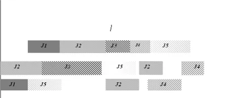
Example: A scheduling situation with 3 work centers and 5 work pieces is considered. There are 14 operations and the chromosomes consist of 14 genes.
Jobs 1 2 3 4 5
Operation 1 2 1 2 3 4 1 2 1 2 3 1 2 3
Machine 1 3 2 3 1 2 2 1 3 1 2 2 1 3
Represen-tation 1 2 3 4 5 6 7 8 9 10 11 12 13 14
Based on the representation above, a sample feasible chromosome will be as follows.
1 3 2 7 4 9 12 13 5 6 8 14 10 11
This representation shows the first scheduled operation is the first operation of the first job on the first machine. The second operation is the first operation of the second job that should be scheduled on the second machine. The third operation is the second operation of the first job that should go on machine three. The other genes can be defined in the same way. The Gantt chart for this representation is depicted in Fig. 1. This schedule is not the output of the proposed GA. In this algorithm, one module is considered that tries to generate schedule from any given chromosome like above. This module takes a cell situation in terms of resource status into account. In other words, AGV location, machines availability and
number of jobs waiting before each machine are considered.
Figure 1. Gantt chart for the given example
Fitness function: Each generated individual is evaluated for its makespan and maximum tardiness if the completion time of job i is defined by:
∑
=
j ij
i O
C
If diis the respective due date, then its tardiness
is computed by Ti=max
(
0,di−Ci)
.Then, the maximum tardiness is the maximum of absolute deviation of jobs from their due dates. Mathematically, the maximum tardiness is computed by Tmax =maxTi. The maximum completion time (i.e., makespan) is defined by:
(
C Cn)
Cmax=max 1,K,
The above criteria or objectives are combined into one to form the objective of the scheduling problem. This combination as mentioned earlier forms the weighted-sum objective function as follows:
( )
s wT( )
SC w
z= c max + t max
where, wc+wt=1. In this paper, both objectives
have equal importance (i.e., wc=wt=0.5).
(or near-optimal) solution. There are three operators, namely reproduction or selection, crossover and mutation [15].
Crossover: The technique used here to cross over two chromosomes is named job-based crossover, which never violates precedence relations between operations [15, 34, 37]. Based on this scheme, once two chromosomes are selected as parents, a job is randomly selected, and its corresponding operations are directly copied into respective positions of offspring. This method guarantees that precedence relations are not violated. Then the remaining unfilled positions are fulfilled with operations of another parent. The following example clarifies the above method.
Example: Chromosomes selected for crossover are as follows:
P1: 1 5 8 2 6 9 3 7 10 4
P2: 5 8 1 9 2 3 6 10 7 4
Let the selected job is 2 and the corresponding operations of job 2 are 5, 6 and 7.
P1: 1 5 8 2 6 9 3 7 10 4
P1: 1 5 8 2 6 9 3 7 10 4
Exchanging operations of job 2 result in the following offspring:
O1: 5 1 8 2 9 3 6 10 7 4
O1: 5 1 8 2 9 3 6 10 7 4
As can be seen, the resulting offspring are feasible. This is mainly because during crossover procedure, the precedence relations are taken into consideration.
Mutation: In this paper, the operation swap mutation is used. Two random positions on the chromosome are chosen and operations associated with these positions are swapped. This mutation may cause infeasibilities in terms of the
precedence relations and a repair function is used to eliminate any such infeasibility [10, 15]. Repair function: A repair function is used to see that the chromosomes do not violate the precedence constraints [22]. The following four-step procedure outlines the repair function in details:
Step 1: Find positions of the operations that violate the precedence relations.
Step 2: Compute the distance between violating operations.
Step 3: If the distance between them is less than half the chromosome length, then swap the operations, else go to Step 4.
Step 4: Randomly pick any one operation and insert it before or after the other depending on the precedence.
Selection: The method used here is known as roulette wheel approach that is commonly used in practice [37]. It belongs to the fitness-proportional selection and can select a new population with respect to the probability distribution based on fitness values (i.e., the more fitted a chromosome is, the more chance it has to be selected).
Here it is required to adapt the selection method in such a way that the minimum objective function receives a higher chance to be selected. For this purpose, a normalization technique based on a scaling method is used [37]. For a minimization problem, this normalization is computed by:
α α
+ −
+ − = ′
min max
max
f f
f f
f k
k
where, fk′ is the normalized fitness function, and max
f and fminare maximum and minimum fitness function values of chromosomes in the current population, respectively.
The just produced fitness values for the current generation are used to select chromosomes based on the roulette wheel approach. This approach gives to each chromosome in the population an opportunity proportionate to its fitness. This probability is calculated by:
( )
∑
∈′ ′ =
Pop k
k k
Population and parameters: The initial population is randomly generated. The number of chromosomes in each generation, crossover and mutation rates, and also the number of generation that algorithm should run to give a satisfying solution are regarded as GA parameters. These parameters must be initialized at the beginning of the GA run.
Termination criteria: Since every heuristic method does not guarantee an optimum value for the problem, an approach is needed to terminate that heuristic method. There are different methods to terminate a heuristic method for an optimization problem. One used here is the number of iteration that the algorithm is run.
5.3. Schedule Generator Apart from the GA methodology, to evaluate each string or solution it is needed to schedule jobs on different machines considering problem constraints. Dispatching algorithms are widely used for scheduling in industrial practice. The algorithms are based on various dispatching rules that prioritize the products for assignment to machines and AGVs. So, in this paper, dispatching rules are incorporated to GA to schedules jobs on machines and AGV. For doing so, four dispatching rules are considered. The main idea behind this is to consider all resources in FMSs. Since our objective function is due date-related, it is worthy to consider a method that attempts to reduce jobs completion time as much as possible, which based on the due date tightness can reduce job tardiness. So as mentioned earlier, the proposed GA is the hybrid one that incorporates priority dispatching rules to do the scheduling task. To keep track of scheduling in terms of the tardiness objective, job slack [38] is computed by:
(
,0)
maxd p t
MS= j− ijm−
This rule is not regarded as those imbedded into the proposed GA. The main goal is to schedule machines in such a way that once a machine becomes free, this index is calculated. Based on this index, the next operation in the current chromosome is scheduled.
These four priority rules are the earliest finishing (or completion) time (EFT), shortest processing time (SPT), shortest distance time
(SDT) and fewest waiting jobs for machine (FWJM). The first two rules focus on jobs, the third one tries to handle the AGV constraint and make use of its availability and its impact on the objective functions. The last one plays a same role as the previous one, excepting that it considers machines buffers.
This proposed methodology works as follows. First, a job with the earliest finishing time is selected to be processed on the corresponding machine. If there is more than one job, the job with the shortest processing time for its subsequent operation is selected. Then tie is broken by considering the distance each job should travel (i.e., the shortest path is selected first by an AGV). If again there is a tie, another PDR is taken into account. Based on this rule, the number of jobs in the target machine buffer determines which job should go first.
This GA in conjunction with the proposed heuristic approach constructs the methodology presented for scheduling jobs and AGV in an FMC.
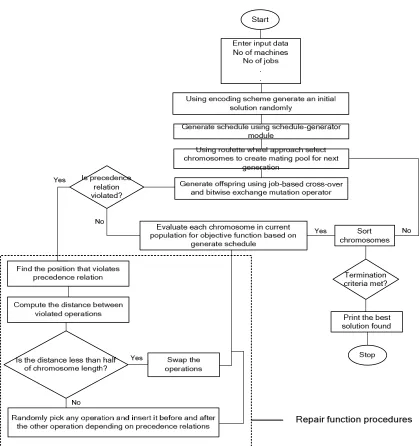
5.4. GA Steps for Scheduling FMC In this section, steps for FMC scheduling are presented bellow.
Step 1: Enter the input data including number of machines, distance between machines, number of jobs and corresponding operations, processing and setup times, and due dates. Then, enter GA parameters, such as population size, crossover and mutation rates, and termination criteria.
Step 2: Randomly generate an initial population using the encoding scheme.
Step 3: Generate schedules using schedule-generator module.
Step 4: Select chromosomes by using the roulette wheel approach to create mating pool for the next generation.
Step 5: Generate offspring population using job-based crossover and bit-wise exchange mutation operators. If some precedence relations are violated, go to Step 6; otherwise, go to Step 7.
Step 6: In case of any violation as a mutation result, run a repair function as described above and then go to Step 7.
Step 8: Sort chromosomes based on the fitness function value.
Step 9: If the termination criterion is met, then stop and print the fittest chromosome as the best solution found so far; otherwise, go to Step 4 for the next generation.
The above-mentioned steps of this algorithm are schematically depicted in Fig. 2. The next section presents the related results of the proposed approach to deal with the scheduling problem in FMC environment.
6. NUMERICAL EXAMPLES AND COMPARISON RESULTS
In this section, the proposed HGA is applied to schedule an FMC with varying parameters. Many problems with different parameters and values are considered and solved. The related results are tabulated. Since the problem environment is somehow similar to the one considered by Liu and MacCarthy [1], the MILP is solved by the Lingo software and the associated results are compared with those of our heuristic approach.
First, ten test problems are randomly generated and shown in Table 1. In each instance, different job sets with different operations are considered. Based on the mathematical formulation, a number of variables and constraints are also calculated, and provided in this table. To further study of the efficiency of the proposed model, different problems with different configurations are defined in three stages, which based on them; both the mathematical model and the GA methodology are applied.
First, FMC with two machines is considered and the problem size is iteratively increased by adding job with varying operations. Processing times are randomly generated from the uniform distribution function, accordingly jobs due dates are defined. This is regarded as Case 1. Then, configurations of the FMC are changed in terms of distance between machines (Case 2), buffer size (Case 3), and speed of AGV (Case 4), respectively. In this paper, only one of the best and complicated cases (i.e., Case 4) is selected and its parameters are set. The remaining cases, the GA parameters are remained unchanged.
TABLE 1. Data for the experimental study
No. of Cons. No. of Var.
Machines Total Oper.
Oper. per job Jobs
Prob. no
596 208
2 8
2 4
1
985 632
2 12
2 6
2
4466 3732
2 30
3 10
3
4561 5336
2 36
6 6
4
6308 7233
2 42
6 7
5
10186 8297
2 45
3 15
6
19648 11891
2 54
6 9
7
13241 14652
2 60
6 10
8
30436 32777
2 90
6 15
9
54681 58102
2 120
6 20
10
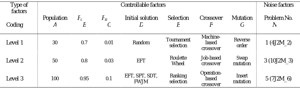
TABLE 2. Experiment factors and their levels
Type of factors
Controllable factors Noise factors
Population Pc Pm Initial solution Selection Crossover Mutation Problem No.
Coding A B C D E F G N
Level 1 30 0.7 0.01 Random Tournament
selection
Machine-based crossover
Reverse
order 1 (4J2M_2)
Level 2 50 0.8 0.03 EFT Roulette
Wheel
Job-based crossover
Swap
mutation 3 (10J2M_3)
Level 3 100 0.95 0.1 EFT, SPT, SDT,
FWJM
Ranking selection
Operation-based crossover
Insert
Figure 2. Flowchart for the proposed hybrid genetic algorithm
6.1. Parameter Setting in the HGA We know that an appropriate selection of parameters and operators has remarkably influence on the efficiency of HGA. In this regard, designing the HGA parameters and operators highly depends on the problem. But, researchers often set these parameters manually according to the related literature. So, in this section, Taguchi experimental design is utilize as a systematic parameter design research method for setting the parameters of the HGA effectively. In this method, controllable factors are placed in an inner orthogonal array and noise factors in the outer orthogonal array [39]. Consequently, the measured
values of quality characteristics are converted into a signal-to-noise (S/N) ratio. For the details of the Taguchi experimental design, readers can refer to the work done by Mason et al. [39].
Let us determine the research characteristic – anticipating the minimization of the maximum completion time and the maximum tardiness as the objective value. Then the smaller value, the better cost value is. Hence, the S/N ratio should be calculated using Lower-is-Better formula give below.
] 1 [ log 10 /
1 2
∑
=
−
= n
i i y n N
The former formula is derived from the loss function given by:
2 ( )
L y = ×k y
In the following, the controllable factors and levels are defined. This paper considers seven factors that affect the solution quality when the proposed HGA is applied. Furthermore, a level number is assigned to perform the parameter design. Factors and their levels are illustrated in Table 2. The inner and/or outer orthogonal array and the corresponding distribution method are selected. According to seven factors and each factor with its levels, we adopt the L27 inner orthogonal array supported with the L3 outer orthogonal array in order to satisfy the requirements.
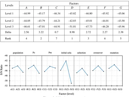
In this section, we provide 27 sets of the experiment results. Each set includes three noise factor combinations and their corresponding S/N ratios. Then, these data convert into the S/N value
and lead to the response table. This table and related graph is depicted in Table 3 and Fig. 3, respectively. As illustrated in Table 3, factor E (i.e., initial solution) is prominent in the performing the HGA. Moreover, the influence of seven factors on minimizing the objective value in the scheduling problem along with the HGA is in the following order.
(1) Initial solution; (2) Crossover rate; (3) Selection method; (4) Population size; (5) Mutation method; (6) Crossover method; (7) Mutation rate.
Since the S/N ratio has the characteristic of the greater the better, the computational results in Table 3 and Fig. 3 indicate the best combination of each factor and level.
TABLE 3. S/N ratio response table
Levels Factors
A B C D E F G
Level 1 –44.99 –45.17 –46.34 –45.82 –46.80 –45.92 –45.06
Level 2 –44.05 –43.79 –44.21 –42.03 –45.01 –44.01 –43.58
Level 3 –46.61 –47.01 –44.91 –51.01 –47.73 –46.28 –45.96
Delta 2.56 3.22 0.7 8.98 2.72 2.27 2.38
Rank 4 2 7 1 3 6 5
Hence, the optimal factor combination is A2: population size = 50; B2: crossover rate = 0.8; C2: mutation rate = 0.03; D2: initial solution = four priority dispatching rules (i.e., EFT, SPT, SDT, FWJM); E2: selection method = roulette wheel; F2: crossover method = job-based crossover; G2: mutation method = swap mutation.
6.2. Algorithm Coding and Results This algorithm is coded in Visual C++ 6 along with the coded MILP model in Lingo 8. Both are run on a PC with 2.6 GHz CPU and the related results are tabulated. The results for this problem are given in Tables 4 to 7 for cases one, two, three and four, respectively.
TABLE 4. Results for Case 1
GA (II) Solution GA Solution
Global Solution Prob.
No Time GAP (%)
(sec.) BOF GAP (%) Time (sec.) BOF Time (sec.) Iterations Optimal 0 50 51.8 5.8 30 54.8 8 8734 51.8 1 0 90 59.9 8.0 67 64.7 17 23075 59.9 2 0 200 30.5 3.8 150 31.65 197 381173 30.5 3 0 600 9 2.8 400 9.25 623 965846 9 4 0 1105 11.5 4.3 964 12 1987 2800953 11.5 5 1.1 1785 27.8 6.7 1630 29.35 3674 3591046 27.5 6 3.2 3256 113 5.5 3180 117.5 6743 7541197 109.5 7 1.2 5824 164 6.8 5342 173 10863 11311795 162 8 2.7 8500 210 6.8 8334 218.5 15642 18664462 204.5 9 2.4 10995 236 6.7 10045 246 24651 35462777 230.5 10
TABLE 5. Results for Case 2
GA (II) Solution GA Solution
Global Solution Prob.
No Time GAP (%)
(sec.) BOF GAP (%) Time (sec.) BOF Time (sec.) Iterations Optimal 0.3 35 52 6.0 20 54.9 8 13998 51.8 1 0.0 150 60 4.2 100 62.5 30 72299 60 2 0.5 605 102 4.9 600 106.5 547 1242305 101.5 3 0.0 990 11.5 13 1012 13 2160 5977290 11.5 4 0.0 2005 16 9.4 1807 17.5 4982 16543810 16 5 1.3 3405 39 5.2 3481 40.5 10030 24815716 38.5 6 2.5 5700 134 8.4 5690 141.5 17642 52113003 130.5 7 4.75 8438 261 11 8519 372 26071 96409055 177 8 - 11000 220 - 11047 224.5 - - - 9 - 13104 276 - 13609 276.5 - - - 10
TABLE 6. Results for Case 3
GA (II) Solution GA Solution
Global Solution Prob.
No Time GAP (%)
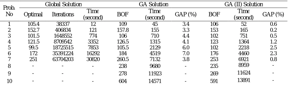
TABLE 7. Results for Case 4
GA (II) Solution GA Solution
Global Solution Prob.
No Time GAP (%)
(second) BOF GAP (%) Time (second) BOF Time (second) Iterations Optimal 0.6 52 106 3.4 45 109 12 38337 105.4 1 0.2 165 153 3.3 155 157.8 121 406834 152.7 2 0.5 751 102 4.4 710 106 774 1648552 101.5 3 1.2 1364 123 4.1 1315 126.5 3352 8709542 121.5 4 2.5 2218 102 6.0 2129 105.5 7853 18725515 99.5 5 2.3 4460 176 7.0 4519 184 16292 35391224 172 6 0.8 6921 253 3.8 7132 260.5 30820 63704203 251 7 - 8959 235 -9680 238 -- - 8 - 11624 269 -11923 278 -- - 9 - 13891 591 -14571 604 -- - 10
It can be concluded that how the configuration and layout of a manufacturing cell can increase the problem complexity. As results show, the use of GAs for solving this problem reduces time needed to get the best objective function dramatically. This shows that the use of this algorithm is promising. It is worth mentioning that FMS layout affects on production planning in general and scheduling in particular (i.e., the more machines are located away, the greater the completion time and tardiness is). For this reason, the cell layout should be considered in the system design and scheduling.
7. CONCLUSIONS AND FUTURE DIRECTIONS
The flexibility is a growing issue in modern industrial firms to respond varying product demands with the short lifecycle. Therefore, new approaches are needed to resolve this issue. Since FMS scheduling problems are NP-hardness, the use of heuristics are quite justified. In this paper, a class of a flexible manufacturing cell (FMS) is considered. A new genetic algorithm (GA)-based approach is proposed to schedule jobs and automated guided vehicle (AGV) for minimizing the maximum tardiness.
The proposed hybrid GA was coded in Visual C++ and run for problems of different sizes. The obtained results were compared with the mathematical model developed by Liu and MacCarthy [1]. As results show, the proposed model outperforms the mixed-integer linear
programming (MILP) model. One reason is worth considering that the required time to solve medium to large-sized problems is a crucial issue in industrial firms.
There are several directions to work on for future study and some are suggested here. One possibility is to apply other heuristic methods separately or in conjunction with GAs. These include, but not limited to, simulated annealing (SA), tabu search (TS) and particle swarm optimization (PSO). Another possibility is to consider a multiple cell system or flexible manufacturing system. In the latter case, other scheduling of a fleet of AGVs can be added to the model. Designing a scheduling system that considers tool management and maintenance activities is another generalization of the problem.
There are other opportunities to extend this paper in future. One of them is to consider the problem in a fuzzy environment or under an uncertainty condition in order to make it as close to real case as possible. Since the considered problem deals with a manufacturing system, integrating this problem with production planning in a more aggregated level is another opportunity for future research.
8. ACKNOWLEDGMENT
of a hybrid genetic algorithm for scheduling a multi-objective flexible manufacturing cells”, which was financially supported by Islamic Azad University – South Tehran Branch.
9.
REFERENCES
1. Liu, J. and MacCarthy, B. L., “A global MILP Model for FMS Scheduling”, European Journal of Operational Research, Vol. 100, (1997), 441–453. 2. Kim, Y. D., “A comparison of dispatching rules for job
shops with multiple identical jobs and alternative routings”, International Journal of Production Research, Vol. 28, No. 5, (1990), 953–962.
3. Srinoi, P., Shayan, E. and Ghotb, F., “A fuzzy logic modeling of dynamic scheduling in FMS”,
International of Journal Production Research, Vol. 44, No. 11, (2006), 2183–2203.
4. Groover, M. P., “Automation, Production Systems, and Computer-Integrated Manufacturing”, 3rd ed., Prentice Hall Inc, (2007).
5. Kim, K. W., Yamazaki, G., Lin, L. and Gen, M., “Network–based hybrid genetic algorithm for scheduling in FMS environments”, Artificial and Life Robotics, Vol. 8, (2004), 67–76.
6. MacCarthy, B. L. and Liu, J., “A new classification for flexible manufacturing systems”, International Journal of Production Research, Vol. 31, No. 2, (1993), 299– 309.
7. Tavakkoli-Moghaddam, R. and Mehdizadeh, E., “A new ILP model for identical parallel-machine scheduling with family setup times minimizing the total weighted flow time by a genetic algorithm”,
International Journal of Engineering, Vol. 20, No. 2, (2007), 183–194.
8. Tavakkoli-Moghaddam, R., Taheri, F. and Bazzazi, M., “Multiobjective unrelated parallel machine scheduling with sequence-dependent setup times and precedence constraints”, International Journal of Engineering, Vol. 21, No. 3, (2008), 269–278.
9. Jerald, J. P., Asokan, R., Saravanan and Rani, A. D. C., “Simultaneous scheduling of parts and automated guided vehicles in an FMS environment using adaptive genetic algorithm”, International of Journal Advanced Manufacturing Technology, Vol. 29, No. 5, (2005), 584–589.
10. Sankar, S. S., Ponnambalam, S. G. and Rajendran, C., “A multi-objective genetic algorithm for scheduling a flexible manufacturing system”, International Journal of Advanced Manufacturing Technology, Vol. 22, No. 3-4, (2005), 229–236.
11. Lee, S. M. and Jung, H. J., “A multiobjective production planning model in a flexible manufacturing environment”, International Journal of Production Research, Vol. 27, No. 11, (1989), 1981–1992. 12. Tung, L. F., Lin, L. and Nagi, R., “Multiple-objective
scheduling for the hierarchical control of flexible manufacturing systems”, The International Journal of
Flexible Manufacturing Systems, Vol. 11, (1999), 379–409.
13. Maccarthy, B. L. and Liu, J., “Addressing the gap in scheduling research: a review of optimization and heuristic methods in production scheduling”,
Introduction of Production Research, Vol. 31, No. 1, (1993), 59–79.
14. Chan, F. T. S., Chan, H. K. and Lau, C. W., “The state of the art in simulation study on FMS scheduling: a comprehensive survey”, The International Journal of Advanced Manufacturing Technology, Vol. 19, (2002), 830–849.
15. Reddy, B. S. P. and Rao, C. S. P., “A hybrid multi-objective GA for simultaneous scheduling of machines and AGVs in FMS”, International Journal of Advanced Manufacturing Technology, Vol. 31, No. 5-6, (2005), 602–613.
16. Low, C. and Wu, T. H., “Mathematical modeling and heuristic approaches to operation scheduling problems in an FMS environment”, International Journal of Production Research, Vol. 39, No. 4, (2001), 689–708. 17. Choi, S. H. and Lee, J. S. L., “A sequencing algorithm
for makespan minimization in FMS”, Journal of Manufacturing Technology Management, Vol. 15, No. 3, (2004), 291–297.
18. Sridharan, R. and Babu, A. S., “Multi-level scheduling decisions in a class of FMS using simulation based metamodels”, Journal of Operational Research Society, Vol. 49, (1998), 591–602.
19. Xu, Z. and Randhawa, S., “Evaluation of scheduling strategies for a dynamic job shop in a tool-shared flexible manufacturing environment”, Production Planning & Control, Vol. 9, No. 1, (1998), 74–86. 20. Sabuncuoglu, I. and Karabuk, S., “A beam search-based
algorithm and evaluation of scheduling approaches for flexible manufacturing systems”, IIE Transaction, Vol. 30, (1998), 179–191.
21. Chan, F. T. S. and Chan, H. K., “Dynamic scheduling for a flexible manufacturing system the pre-emptive approach”, International Journal Advanced Manufacturing Technology, Vol. 17, (2001), 760–768. 22. Ulsoy, G., Serifoglu, F. S. and Bilge, U., “A genetic
algorithm approach to the simultaneous scheduling of machines and automated guided vehicles”, Computers & Operations Research, Vol. 24, No. 4, (1997), 335– 351.
23. Logendran, R. and Sonthinen, A., “A tabu search-based approach for scheduling job-shop type flexible manufacturing systems”, Journal of Operation Research Society, Vol. 48, (1997), 264–277.
24. Noorul Haq, A., Karthikeyan, T. and Dinesh, M., “Scheduling decision in FMS using a heuristic approach”, International Journal of Advanced Manufacturing Technology, Vol. 22, No. 5-6, (2003), 374–379.
25. Sakawa, M., “Genetic algorithms and fuzzy multi-objective optimization”, Kluwer Academic Publisher, (2001).
26. Baker, K. R., “Introduction to sequencing and scheduling”, John Wiley & Sons, New York, (1974). 27. Prabaharan, T., Nakkeeran, P. R. and Jawahar, N.,
Advanced Manufacturing Technology, Vol. 29, (2006), 729–745.
28. Deb, K., “Multi-objective optimization using evolutionary algorithms”, Chichester, UK Wiley, (2001).
29. Mezura-Montes, E., Coello Coello, C.A., “Use of multi-objective optimization concepts to handle constraints in genetic algorithm, in: Abraham, A., Jain, L., and Goldberg, R. (Eds), Evolutionary Multi-objective optimization: Theoretical advances and applications”, Springer, (2005).
30. Ehrgott, M., “Multi-criteria optimization”, Springer, Berlin-Heidelberg, (2005).
31. Evans, G. W., “An overview of techniques for solving multi-objective mathematical programs”, Management Science, Vol. 30, (1984), 1268–1282.
32. Fry, T. D., Armstrong, R. D. and Lewis, H., “A framework for single machine multiple objective sequencing research”, Omega, Vol. 17, (1989), 595– 607.
33. Coello Coello, C.A., Van Veldhuizen, D.A., and Lamount, G.B., “Evolutionary algorithm for solving
multi-objective problems”, Kluwer Academic Publishers, New York, (2002).
34. Gen, M. and Cheng, R., “Genetic algorithms and engineering optimization”, John Wiley & Sons, New York, (2000).
35. Cheng, R. and Gen, M., “A survey of genetic multi-objective optimization”, Technical Report, Ashikaga Institute of Technology, (1998).
36. Bilge, U. and Ulusoy, G., “A time window approach to simultaneous scheduling of machines and material handling system in an FMS”, Operations Research, Vol. 43, No 6, (1995), 1058-1070.
37. Gen, M. and Cheng, R., “Genetic algorithms and engineering design”, John Wiley & Sons, New York, (1997).