Data-driven Rank Breaking for Efficient Rank Aggregation
Ashish Khetan [email protected]
Sewoong Oh [email protected]
Department of Industrial and Enterprise Systems Engineering University of Illinois at Urbana-Champaign
Urbana, IL 61801, USA
Editor:Benjamin Recht
Abstract
Rank aggregation systems collect ordinal preferences from individuals to produce a global ranking that represents the social preference. Rank-breaking is a common practice to reduce the com-putational complexity of learning the global ranking. The individual preferences are broken into pairwise comparisons and applied to efficient algorithms tailored for independent paired compar-isons. However, due to the ignored dependencies in the data, naive rank-breaking approaches can result in inconsistent estimates. The key idea to produce accurate and consistent estimates is to treat the pairwise comparisons unequally, depending on the topology of the collected data. In this paper, we provide the optimal rank-breaking estimator, which not only achieves consistency but also achieves the best error bound. This allows us to characterize the fundamental tradeoff between accuracy and complexity. Further, the analysis identifies how the accuracy depends on the spectral gap of a corresponding comparison graph.
Keywords: Rank aggregation, Plackett-Luce model, Sample complexity
1. Introduction
In several applications such as electing officials, choosing policies, or making recommendations, we are given partial preferences from individuals over a set of alternatives, with the goal of producing a global ranking that represents the collective preference of the population or the society. This process is referred to as rank aggregation. One popular approach islearning to rank. Economists have modeled each individual as a rational being maximizing his/her perceived utility. Parametric probabilistic models, known collectively as Random Utility Models (RUMs), have been proposed to model such individual choices and preferences (McFadden, 1980). This allows one to infer the global ranking by learning the inherent utility from individuals’ revealed preferences, which are noisy manifestations of the underlying true utility of the alternatives.
Traditionally, learning to rank has been studied under the following data collection scenarios: pairwise comparisons, best-out-of-k comparisons, and k-way comparisons. Pairwise comparisons
a ranked list over a set ofk items. In some real-world elections, voters provide ranked preferences over the whole set of candidates (Lundell, 2007). We refer to these three types of ordinal data collection scenarios as ‘traditional’ throughout this paper.
For such traditional data sets, there are several computationally efficient inference algorithms for finding the Maximum Likelihood (ML) estimates that provably achieve the minimax optimal performance (Negahban et al., 2012; Shah et al., 2015a; Hajek et al., 2014). However, modern data sets can be unstructured. Individual’s revealed ordinal preferences can be implicit, such as movie ratings, time spent on the news articles, and whether the user finished watching the movie or not. In crowdsourcing, it has also been observed that humans are more efficient at performing batch comparisons (Gomes et al., 2011), as opposed to providing the full ranking or choosing the top item. This calls for more flexible approaches for rank aggregation that can take such diverse forms of ordinal data into account. For such non-traditional data sets, finding the ML estimate can become significantly more challenging, requiring run-time exponential in the problem parameters. To avoid such a computational bottleneck, a common heuristic is to resort to rank-breaking. The collected ordinal data is first transformed into a bag of pairwise comparisons, ignoring the dependencies that were present in the original data. This is then processed via existing inference algorithms tailored for independent pairwise comparisons, hoping that the dependency present in the input data does not lead to inconsistency in estimation. This idea is one of the main motivations for numerous approaches specializing in learning to rank from pairwise comparisons, e.g., (Ford Jr., 1957; Negahban et al., 2014; Azari Soufiani et al., 2013). However, such a heuristic of full rank-breaking defined explicitly in (1), where all pairwise comparisons are weighted and treated equally ignoring their dependencies, has been recently shown to introduce inconsistency (Azari Soufiani et al., 2014).
The key idea to produce accurate and consistent estimates is to treat the pairwise comparisons unequally, depending on the topology of the collected data. A fundamental question of interest to practitioners is how to choose the weight of each pairwise comparison in order to achieve not only consistency but also the best accuracy, among those consistent estimators using rank-breaking. We study how the accuracy of resulting estimate depends on the topology of the data and the weights on the pairwise comparisons. This provides a guideline for the optimal choice of the weights, driven by the topology of the data, that leads to accurate estimates.
Problem formulation. The premise in the current race to collect more data on user activities is that, a hidden true preference manifests in the user’s activities and choices. Such data can be explicit, as in ratings, ranked lists, pairwise comparisons, and like/dislike buttons. Others are more implicit, such as purchase history and viewing times. While more data in general allows for a more accurate inference, the heterogeneity of user activities makes it difficult to infer the underlying preferences directly. Further, each user reveals her preference on only a few contents.
Traditional collaborative filtering fails to capture the diversity of modern data sets. The sparsity and heterogeneity of the data renders typical similarity measures ineffective in the nearest-neighbor methods. Consequently, simple measures of similarity prevail in practice, as in Amazon’s “people who bought ... also bought ...” scheme. Score-based methods require translating heterogeneous data into numeric scores, which is a priori a difficult task. Even if explicit ratings are observed, those are often unreliable and the scale of such ratings vary from user to user.
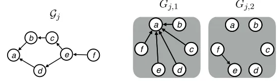
use in revealed preference theory). We interpret user activities as manifestation of the hidden preferences according to discrete choice models (in particular the Plackett-Luce model defined in (1)). This provides a more reliable, scale-free, and widely applicable representation of the heterogeneous data as partial orderings, as well as a probabilistic interpretation of how preferences manifest. In full generality, the data collected from each individual can be represented by apartially ordered set (poset). Assuming consistency in a user’s revealed preferences, any ordered relations can be seamlessly translated into a poset, represented as a Hasse diagram by a directed acyclic graph (DAG). The DAG below represents ordered relationsa >{b, d},b > c,{c, d}> e, ande > f. For example, this could have been translated from two sources: a five star rating onaand a three star ratings on b, c, d, a two star rating on e, and a one star rating on f; and the item b being purchased after reviewing cas well.
a
b c
e
d
f Gj
a b
c
e d f
a b
c
e d f
a b
c
e d f
a b
c
e d f
Gj,1 Gj,2
Figure 1: A DAG representation of consistent partial ordering of a user j, also called a Hasse diagram (left). A set of rank-breaking graphs extracted from the Hasse diagram for the separator itemaand e, respectively (right).
There are n users or agents, and each agent j provides his/her ordinal evaluation on a subset
Sj of d items or alternatives. We refer to Sj ⊂ {1,2, . . . , d} as offerings provided to j, and use κj =|Sj|to denote the size of the offerings. We assume that the partial ordering over the offerings
is a manifestation of her preferences as per a popular choice model known as Plackett-Luce (PL) model. As we explain in detail below, the PL model produces total orderings (rather than partial ones). The data collector queries each user for a partial ranking in the form of a poset over Sj.
For example, the data collector can ask for the top item, unordered subset of three next preferred items, the fifth item, and the least preferred item. In this case, an example of such poset could be a <{b, c, d}< e < f, which could have been generated from a total ordering produced by the PL model and taking the corresponding partial ordering from the total ordering. Notice that we fix the topology of the DAG first and ask the user to fill in the node identities corresponding to her total ordering as (randomly) generated by the PL model. Hence, the structure of the poset is considered deterministic, and only the identity of the nodes in the poset is considered random. Alternatively, one could consider a different scenario where the topology of the poset is also random and depends on the outcome of the preference, which is out-side the scope of this paper and provides an interesting future research direction.
The PL model is a special case of random utility models, defined as follows (Walker and Ben-Akiva, 2002; Azari Soufiani et al., 2012). Each item i has a real-valued latent utility θi. When
properties, making this model realistic in various domains, including marketing (Guadagni and Little, 1983), transportation (McFadden, 1980; Ben-Akiva and Lerman, 1985), biology (Sham and Curtis, 1995), and natural language processing (Mikolov et al., 2013). Precisely, each userj, when presented with a set Sj of items, draws a noisy utility of each item iaccording to
ui = θi+Zi ,
where Zi’s follow the independent standard Gumbel distribution. Then we observe the ranking resulting from sorting the items as per noisy observed utilitiesuj’s. Alternatively, the PL model is
also equivalent to the following random process. For a set of alternativesSj, a rankingσj : [|S|]→S
is generated in two steps: (1) independently assign each item i ∈ Sj an unobserved value Xi, exponentially distributed with mean e−θi; (2) select a ranking σ
j so thatXσj(1) ≤Xσj(2) ≤ · · · ≤ Xσj(|Sj|).
The PL model (i) satisfies Luce’s ‘independence of irrelevant alternatives’ in social choice the-ory (Ray, 1973), and has a simple characterization as sequential (random) choices as explained below; and (ii) has a maximum likelihood estimator (MLE) which is a convex program in θin the traditional scenarios of pairwise, best-out-of-kand k-way comparisons. Let P(a >{b, c, d}) denote
the probabilityawas chosen as the best alternative among the set{a, b, c, d}. Then, the probability that a user reveals a linear order (a > b > c > d) is equivalent as making sequential choice from the top to bottom:
P(a > b > c > d) = P(a >{b, c, d})P(b >{c, d}) P(c > d)
= e
θa
(eθa+eθb+eθc+eθd)
eθb
(eθb+eθc+eθd)
eθc
(eθc+eθd) .
We use the notation (a > b) to denote the event that ais preferred over b. In general, for user j
presented with offerings Sj, the probability that the revealed preference is a total ordering σj is
P(σj) = Qi∈{1,...,κj−1}(e θσ−1(i)
)/(Pκj
i0=ieθσ−1(i0)). We consider the true utility θ∗ ∈ Ωb, where we
define Ωb as
Ωb ≡ n
θ∈Rd
X
i∈[d]
θi = 0,|θi| ≤bfor all i∈[d] o.
Note that by definition, the PL model is invariant under shifting the utility θi’s. Hence, the centering ensures uniqueness of the parameters for each PL model. The bound b on the dynamic range is not a restriction, but is written explicitly to capture the dependence of the accuracy in our main results.
We have n users each providing a partial ordering of a set of offeringsSj according to the PL model. Let Gj denote both the DAG representing the partial ordering from user j’s preferences. With a slight abuse of notations, we also let Gj denote the set of rankings that are consistent
with this DAG. For general partial orderings, the probability of observingGj is the sum of all total
orderings that is consistent with the observation, i.e. P(Gj) =Pσ∈GjP(σ). The goal is to efficiently
learn the true utility θ∗ ∈ Ωb, from the n sampled partial orderings. One popular approach is to
compute the maximum likelihood estimate (MLE) by solving the following optimization:
maximize
θ∈Ωb
n X
j=1
This optimization is a simple convex optimization, in particular a logit regression, when the struc-ture of the data {Gj}j∈[n] is traditional. This is one of the reasons the PL model is attractive. However, for general posets, this can be computationally challenging. Consider an example of position-p ranking, where each user provides which item is at p-th position in his/her ranking. Each term in the log-likelihood for this data involves summation over O((p−1)!) rankings, which takesO(n(p−1)!) operations to evaluate the objective function. Since pcan be as large asd, such a computational blow-up renders MLE approach impractical. A common remedy is to resort to rank-breaking, which might result in inconsistent estimates.
Rank-breaking. Rank-breaking refers to the idea of extracting a set of pairwise comparisons from the observed partial orderings and applying estimators tailored for paired comparisons treating each piece of comparisons as independent. Both the choice of which paired comparisons to extract and the choice of parameters in the estimator, which we callweights, turns out to be crucial as we will show. Inappropriate selection of the paired comparisons can lead to inconsistent estimators as proved in Azari Soufiani et al. (2014), and the standard choice of the parameters can lead to a significantly suboptimal performance.
A naive rank-breaking that is widely used in practice is to apply rank-breaking to all possible pairwise relations that one can read from the partial ordering and weighing them equally. We refer to this practice asfull rank-breaking. In the example in Figure 1, full rank-breaking first extracts the bag of comparisons C={(a > b),(a > c),(a > d),(a > e),(a > f), . . . ,(e > f)}with 13 paired comparison outcomes, and apply the maximum likelihood estimator treating each paired outcome as independent. Precisely, the full rank-breaking estimatorsolves the convex optimization of
b
θ ∈ arg max
θ∈Ωb
X
(i>i0)∈C
θi−logeθi+eθi0
. (1)
There are several efficient implementation tailored for this problem (Ford Jr., 1957; Hunter, 2004; Negahban et al., 2012; Maystre and Grossglauser, 2015a), and under the traditional scenarios, these approaches provably achieve the minimax optimal rate (Hajek et al., 2014; Shah et al., 2015a). For general non-traditional data sets, there is a significant gain in computational complexity. In the case of position-p ranking, where each of the n users report his/her p-th ranking item among κ
items, the computational complexity reduces fromO(n(p−1)!) for the MLE in (1) toO(n p(κ−p)) for the full rank-breaking estimator in (1). However, this gain comes at the cost of accuracy. It is known that the full-rank breaking estimator is inconsistent (Azari Soufiani et al., 2014); the error is strictly bounded away from zero even with infinite samples.
Perhaps surprisingly, Azari Soufiani et al. (2014) recently characterized the entire set of con-sistent rank-breaking estimators. Instead of using the bag of paired comparisons, the sufficient information for consistent rank-breaking is a set of rank-breaking graphs defined as follows.
Recall that a userjprovides his/her preference as a poset represented by a DAGGj. Consistent rank-breaking first identifies all separators in the DAG. A node in the DAG is a separator if one can partition the rest of the nodes into two parts. A partition Atop which is the set of items that are preferred over the separator item, and a partition Abottom which is the set of items that are
less preferred than the separator item. One caveat is that we allow Atop to be empty, butAbottom
the name separator. We use`j to denote the number of separators in the posetGj from userj. We
let pj,a denote the ranked position of thea-th separator in the posetGj, and we sort the positions
such that pj,1 < pj,2 < . . . < pj,`j. The set of separators is denoted by Pj ={pj,1, pj,2,· · ·, pj,`j}.
For example, since the separator a is ranked at position 1 and e is at the 5-th position, `j = 2, pj,1 = 1, andpj,2 = 5. Note thatf is not a separator (whereasais) since corresponding Abottom is
empty.
Conveniently, we represent this extracted partial ordering using a set of DAGs, which are called
rank-breaking graphs. We generate one rank-breaking graph per separator. A rank breaking graph
Gj,a = (Sj, Ej,a) for user j and the a-th separator is defined as a directed graph over the set of
offerings Sj, where we add an edge from a node that is less preferred than the a-th separator to the separator, i.e. Ej,a = {(i, i0)|i0 is the a-th separator, andσ−j1(i) > pj,a}. Note that by the definition of the separator,Ej,a is a non-empty set. An example of rank-breaking graphs are shown
in Figure 1.
This rank-breaking graphs were introduced in Azari Soufiani et al. (2013), where it was shown that the pairwise ordinal relations that is represented by edges in the rank-breaking graphs are sufficient information for using any estimation based on the idea of rank-breaking. Precisely, on the converse side, it was proved in Azari Soufiani et al. (2014) that any pairwise outcomes that is not present in the rank-breaking graphs Gj,a’s lead to inconsistency for a general θ∗. On the achievability side, it was proved that all pairwise outcomes that are present in the rank-breaking graphs give a consistent estimator, as long as all the paired comparisons in each Gj,a are weighted
equally.
It should be noted that rank-breaking graphs are defined slightly differently in Azari Soufiani et al. (2013). Specifically, Azari Soufiani et al. (2013) introduced a different notion of rank-breaking graph, where the vertices represent positions in total ordering. An edge between two vertices i1
andi2 denotes that the pairwise comparison between items ranked at positioni1 andi2 is included in the estimator. Given such observation from the PL model, Azari Soufiani et al. (2013) and Azari Soufiani et al. (2014) prove that a rank-breaking graph is consistent if and only if it satisfies the following property. If a vertexi1 is connected to any vertexi2, wherei2 > i1, theni1 must be connected to all the verticesi3 such thati3> i1. Although the specific definitions of rank-breaking graphs are different from our setting, the mathematical analysis of Azari Soufiani et al. (2013) still holds when interpreted appropriately. Specifically, we consider only those rank-breaking that are consistent under the conditions given in Azari Soufiani et al. (2013). In our rank-breaking graph
Gj,a, a separator node is connected to all the other item nodes that are ranked below it (numerically
higher positions).
In the algorithm described in (33), we satisfy this sufficient condition for consistency by re-stricting to a class of convex optimizations that use the same weight λj,a for all (κ−pj,a) paired comparisons in the objective function, as opposed to allowing more general weights that defer from a pair to another pair in a rank-breaking graph Gj,a.
Algorithm. Consistent rank-breaking first identifies separators in the collected posets{Gj}j∈[n]
rank-breaking estimatorsolves the convex optimization of maximizing the paired log likelihoods
LRB(θ) =
n X
j=1 `j
X
a=1 λj,a
n X
(i,i0)∈E
j,a
θi0−log
eθi+eθi0
o
, (2)
where Ej,a’s are defined as above via separators and different choices of the non-negative weights λj,a’s are possible and the performance depends on such choices. Each weightλj,a determine how
much we want to weigh the contribution of a corresponding rank-breaking graph Gj,a. We define theconsistent rank-breaking estimate θbas the optimal solution of the convex program:
b
θ ∈ arg max
θ∈Ωb
LRB(θ). (3)
By changing how we weigh each rank-breaking graph (by choosing the λj,a’s), the convex program
(3) spans the entire set of consistent rank-breaking estimators, as characterized in Azari Soufiani et al. (2014). However, only asymptotic consistency was known, which holds independent of the choice of the weightsλj,a’s. Naturally, a uniform choice ofλj,a=λwas proposed in (Azari Soufiani
et al., 2014).
Note that this can be efficiently solved, since this is a simple convex optimization, in particular a logit regression, with only O(Pn
j=1 `jκj) terms. For a special case of position-p breaking, the O(n(p −1)!) complexity of evaluating the objective function for the MLE is now significantly reduced to O(n(κ−p)) by rank-breaking. Given this potential exponential gain in efficiency, a natural question of interest is “what is the price we pay in the accuracy?”. We provide a sharp analysis of the performance of rank-breaking estimators in the finite sample regime, that quantifies the price of rank-breaking. Similarly, for a practitioner, a core problem of interest is how to choose the weights in the optimization in order to achieve the best accuracy. Our analysis provides a data-driven guideline for choosing the optimal weights.
Contributions. In this paper, we provide an upper bound on the error achieved by the rank-breaking estimator of (3) for any choice of the weights in Theorem 8. This explicitly shows how the error depends on the choice of the weights, and provides a guideline for choosing the optimal weights λj,a’s in a data-driven manner. We provide the explicit formula for the optimal choice
of the weights and provide the the error bound in Theorem 2. The analysis shows the explicit dependence of the error in the problem dimension d and the number of users nthat matches the numerical experiments.
If we are designing surveys and can choose which subset of items to offer to each user and also can decide which type of ordinal data we can collect, then we want to design such surveys in a way to maximize the accuracy for a given number of questions asked. Our analysis provides how the accuracy depends on the topology of the collected data, and provides a guidance when we do have some control over which questions to ask and which data to collect. One should maximize the spectral gap of corresponding comparison graph. Further, for some canonical scenarios, we quantify the price of breaking by comparing the error bound of the proposed data-driven rank-breaking with the lower bound on the MLE, which can have a significantly larger computational cost (Theorem 4).
associated with each item. θ∗ represents true utility andθbdenotes the estimated utility. We usen
to denote the number of users/agents and index each user byj∈ {1,2, . . . , n}. Sj ⊆ {1, . . . , d}refer
to the offerings provided to the j-th user and we use κj =|Sj| to denote the size of the offerings.
Gj denote the DAG (Hasse diagram) representing the partial ordering from user j’s preferences.
Pj = {pj,1, pj,2,· · ·, pj,`j} denotes the set of separators in the DAG Gj, where pj,1,· · ·, pj,`j are
the positions of the separators, and `j is the number of separators. Gj,a = (Sj, Ej,a) denote the rank-breaking graph for thea-th separator extracted from the partial orderingGj of userj.
For any positive integer N, let [N] ={1,· · · , N}. For a ranking σ over S, i.e.,σ is a mapping from [|S|] to S, let σ−1 denote the inverse mapping.For a vector x, let kxk2 denote the standard l2 norm. Let 1 denote the all-ones vector and 0 denote the all-zeros vector with the appropriate dimension. Let Sd denote the set of d×d symmetric matrices with real-valued entries. For X ∈ Sd, let λ1(X)≤λ2(X)≤ · · · ≤λd(X) denote its eigenvalues sorted in increasing order. Let
Tr(X) =Pd
i=1λi(X) denote its trace and kXk= max{|λ1(X)|,|λd(X)|}denote its spectral norm.
For two matricesX, Y ∈ Sd, we writeXY ifX−Y is positive semi-definite, i.e.,λ
1(X−Y)≥0.
Letei denote a unit vector in Rd along the i-th direction.
2. Comparisons Graph and the Graph Laplacian
In the analysis of the convex program (3), we show that, with high probability, the objective function is strictly concave with λ2(H(θ))≤ −Cbγ λ2(L)< 0 (Lemma 11) for all θ∈ Ωb and the
gradient is bounded by k∇LRB(θ∗)k2 ≤Cb0 q
logdP
j∈[n]`j (Lemma 10). Shortly, we will define γ
andλ2(L), which captures the dependence on the topology of the data, andCb0 andCb are constants that only depend on b. Putting these together, we will show that there exists a θ∈Ωb such that
kθb−θ∗k2 ≤
2k∇LRB(θ∗)k2
−λ2(H(θ)) ≤ C
00
b q
logdP j∈[n]`j γ λ2(L) .
Here λ2(H(θ)) denotes the second largest eigenvalue of a negative semi-definite Hessian matrix
H(θ) of the objective function. The reason the second largest eigenvalue shows up is because the top eigenvector is always the all-ones vector which by the definition of Ωbis infeasible. The accuracy
depends on the topology of the collected data via the comparison graph of given data.
Definition 1. (Comparison graph H). We define a graph H([d], E) where each alternative corre-sponds to a node, and we put an edge (i, i0) if there exists an agent j whose offerings is a set Sj such that i, i0 ∈Sj. Each edge (i, i0)∈E has a weight Aii0 defined as
Aii0 =
X
j∈[n]:i,i0∈S
j `j κj(κj−1) ,
where κj =|Sj|is the size of each sampled set and `j is the number of separators in Sj defined by rank-breaking in Section 1.
Define a diagonal matrix D = diag(A1), and the corresponding graph Laplacian L =D−A, such that
L =
n X
j=1 `j κj(κj−1)
X
i<i0∈S
j
Let 0 = λ1(L) ≤λ2(L) ≤ · · · ≤λd(L) denote the (sorted) eigenvalues of L. Of special interest is λ2(L), also called the spectral gap, which measured how well-connected the graph is. Intuitively,
one can expect better accuracy when the spectral gap is larger, as evidenced in previous learning to rank results in simpler settings (Negahban et al., 2014; Shah et al., 2015a; Hajek et al., 2014). This is made precise in (4), and in the main result of Theorem 2, we appropriately rescale the spectral gap and useα∈[0,1] defined as
α ≡ λ2(L)(d−1)
Tr(L) =
λ2(L)(d−1)
Pn j=1`j
. (5)
The accuracy also depends on the topology via the maximum weighted degree defined asDmax≡
maxi∈[d]Dii = maxi∈[d]{ P
j:i∈Sj`j/κj}. Note that the average weighted degree is
P
iDii/d =
Tr(L)/d, and we rescale it by Dmax such that
β ≡ Tr(L)
dDmax = Pn
j=1`j
dDmax . (6)
We will show that the performance of rank breaking estimator depends on the topology of the graph through these two parameters. The larger the spectral gapα the smaller error we get with the same effective sample size. The degree imbalance β ∈[0,1] determines how many samples are required for the analysis to hold. We need smaller number of samples if the weighted degrees are balanced, which happens if β is large (close to one).
The following quantity also determines the convexity of the objective function.
γ ≡ min
j∈[n] (
1− pj,`j κj
!d2e2be−2)
. (7)
Note thatγ is between zero and one, and a larger value is desired as the objective function becomes more concave and a better accuracy follows. When we are collecting data where the size of the offeringsκj’s are increasing withdbut the position of the separators are close to the top, such that
κj =ω(d) andpj,`j =O(1), then forb=O(1) the above quantityγ can be made arbitrarily close to
one, for large enough problem sized. On the other hand, whenpj,`j is close toκj, the accuracy can
degrade significantly as stronger alternatives might have small chance of showing up in the rank breaking. The value ofγ is quite sensitive tob. The reason we have such a inferior dependence on
b is because we wanted to give a universal bound on the Hessian that is simple. It is not difficult to get a tighter bound with a larger value of γ, but will inevitably depend on the structure of the data in a complicated fashion.
To ensure that the (second) largest eigenvalue of the Hessian is small enough, we need enough samples. This is captured byη defined as
η ≡ max
j∈[n]
{ηj}, where ηj = κj
max{`j, κj−pj,`j}
. (8)
Note that 1< ηj ≤κj/`j. A smaller value ofη is desired as we require smaller number of samples,
as shown in Theorem 2. This happens, for instance, when all separators are at the top, such that
pj,`j = `j and ηj = κj/(κj −`j), which is close to one for large κj. On the other hand, when all
separators are at the bottom of the list, then η can be as large asκj.
3. Main Results
We present the main theoretical results accompanied by corresponding numerical simulations in this section.
3.1 Upper Bound on the Achievable Error
We present the main result that provides an upper bound on the resulting error and explicitly shows the dependence on the topology of the data. As explained in Section 1, we assume that each user provides a partial ranking according to his/her position of the separators. Precisely, we assume the set of offerings Sj, the number of separators `j, and their respective positions Pj ={pj,1, . . . , pj,`j}
are predetermined. Each user draws the ranking of items from the PL model, and provides the partial ranking according to the separators of the form of {a > {b, c, d} > e > f} in the example in the Figure 1.
Theorem 2. Suppose there arenusers, ditems parametrized byθ∗∈Ωb, each userj is presented with a set of offerings Sj ⊆ [d], and provides a partial ordering under the PL model. When the effective sample size Pn
j=1`j is large enough such that
n X
j=1
`j ≥ 2
11e18bηlog(`max+ 2)2
α2γ2β dlogd , (9)
whereb≡maxi|θi∗|is the dynamic range,`max≡maxj∈[n]`j,αis the (rescaled) spectral gap defined in (5),β is the (rescaled) maximum degree defined in (6),γ and η are defined in Eqs. (7)and (8), then the rank-breaking estimatorin (3) with the choice of
λj,a = 1
κj−pj,a
, (10)
for all a∈[`j] andj ∈[n] achieves
1
√
d bθ−θ∗
2 ≤
4√2e4b(1 +e2b)2 αγ
s
dlogd Pn
j=1`j
, (11)
with probability at least 1−3e3d−3.
Consider an ideal case where the spectral gap is large such thatα is a strictly positive constant and the dynamic rangebis finite and maxj∈[n]pj,`j/κj =C for some constantC <1 such thatγ is
also a constant independent of the problem sized. Then the upper bound in (11) implies that we need the effective sample size to scale as O(dlogd), which is only a logarithmic factor larger than the number of parameters to be estimated. Such a logarithmic gap is also unavoidable and due to the fact that we require high probability bounds, where we want the tail probability to decrease at least polynomially ind. We discuss the role of the topology of the data in Section 4.
0.01 0.1 1 10
1 10 100
top- -separators random- -separators among top-half random- -separators
Ckbθ−θ∗k2
2
number of separators `
` `
`
0.01 0.1 1 10
1000 10000 100000
top-16-separators random-16-separators among top-half random-16-separators
sample size n
0.02 0.06 0.1 0.14 0.18
1 200 400 600 800 1024
top-16-separators random-16-separators among top-half random-16-separators
|bθi−θ∗i|
item number
Weak Strong
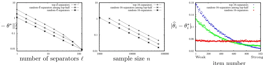
Figure 2: Simulation confirmskθ∗−θbk22 ∝1/(` n), and smaller error is achieved for separators that
are well spread out.
In Figure 2 , we verify the scaling of the resulting error via numerical simulations. We fix
d= 1024 and κj =κ= 128, and vary the number of separators `j =`for fixed n= 128000 (left),
and vary the number of samples n for fixed`j =`= 16 (middle). Each point is average over 100 instances. The plot confirms that the mean squared error scales as 1/(` n). Each sample is a partial ranking from a set ofκ alternatives chosen uniformly at random, where the partial ranking is from a PL model with weights θ∗ chosen i.i.d. uniformly over [−b, b] with b = 2. To investigate the role of the position of the separators, we compare three scenarios. The top-`-separators choose the top`positions for separators, therandom-`-separators among top-halfchoose`positions uniformly random from the top half, and therandom-`-separatorschoose the positions uniformly at random. We observe that when the positions of the separators are well spread out among the κ offerings, which happens forrandom-`-separators, we get better accuracy.
The figure on the right provides an insight into this trend for ` = 16 and n = 16000. The absolute error |θ∗i −θib| is roughly same for each item i ∈ [d] when breaking positions are chosen
uniformly at random between 1 toκ−1 whereas it is significantly higher for weak preference score items when breaking positions are restricted between 1 toκ/2 or are top-`. This is due to the fact that the probability of each item being ranked at different positions is different, and in particular probability of the low preference score items being ranked in top-` is very small. The third figure is averaged over 1000 instances. Normalization constant C is n/d2 and 103`/d2 for the first and
second figures respectively. For the first figure n is chosen relatively large such that n` is large enough even for `= 1.
3.2 The Price of Rank Breaking for the Special Case of Position-p Ranking
Corollary 3. Under the hypotheses of Theorem 2, there exist positive constants C andc that only depend on b such that ifn≥C(ηdlogd)/(α2γ2β) then
1
√
d bθ−θ∗
2 ≤ c αγ
r dlogd
n . (12)
Note that the error only depends on the position p through γ and η, and is not sensitive. To quantify the price of rank-breaking, we compare this result to a fundamental lower bound on the minimax rate in Theorem 4. We can compute a sharp lower bound on the minimax rate, using the Cram´er-Rao bound, and a proof is provided in Section 8.3.
Theorem 4. Let U denote the set of all unbiased estimators of θ∗ and suppose b >0, then
inf
b
θ∈U
sup
θ∗∈Ω
b
E[kθb−θ∗k2] ≥
1 2plog(κmax)2
d X
i=2
1
λi(L)
≥ 1
2plog(κmax)2
(d−1)2
n ,
where κmax= maxj∈[n]|Sj|and the second inequality follows from the Jensen’s inequality.
Note that the second inequality is tight up to a constant factor, when the graph is an expander with a large spectral gap. For expanders, α in the bound (12) is also a strictly positive constant. This suggests that rank-breaking gains in computational efficiency by a super-exponential factor of (p−1)!, at the price of increased error by a factor ofp, ignoring poly-logarithmic factors.
3.3 Tighter Analysis for the Special Case of Top-` Separators Scenario
The main result in Theorem 2 is general in the sense that it applies to any partial ranking data that is represented by positions of the separators. However, the bound can be quite loose, especially whenγ is small, i.e. pj,`j is close toκj. For some special cases, we can tighten the analysis to get a
sharper bound. One caveat is that we use a slightly sub-optimal choice of parametersλj,a = 1/κj
instead of 1/(κj−a), to simplify the analysis and still get the order optimal error bound we want.
Concretely, we consider a special case of top-`separators scenario, where each agent gives a ranked list of her most preferred `j alternatives among κj offered set of items. Precisely, the locations of the separators are (pj,1, pj,2, . . . , pj,`j) = (1,2, . . . , `j).
Theorem 5. Under the PL model, n partial orderings are sampled over d items parametrized by θ∗ ∈ Ωb, where the j-th sample is a ranked list of the top-`j items among the κj items offered to the agent. If
n X
j=1 `j ≥
212e6b
βα2 dlogd , (13)
where b≡maxi,i0|θ∗
i −θi∗0|and α, β are defined in (5) and (6), then therank-breaking estimatorin
(3) with the choice of λj,a= 1/κj for alla∈[`j]and j∈[n] achieves
1
√
d bθ−θ∗
2 ≤
16(1 +e2b)2 α
s
dlogd Pn
j=1`j
, (14)
A proof is provided in Section 8.4. In comparison to the general bound in Theorem 2, this is tighter since there is no dependence in γ orη. This gain is significant when, for example, pj,`j is
close to κj. As an extreme example, if all agents are offered the entire set of alternatives and are asked to rank all of them, such that κj =dand `j =d−1 for allj ∈[n], then the generic bound
in (11) is loose by a factor of (e4b/2√2)dd2e2be−2, compared to the above bound.
In the top-`separators scenario, the data set consists of the ranking among top-`j items of the set Sj, i.e., [σj(1), σj(2),· · ·, σj(`j)]. The corresponding log-likelihood of the PL model is
L(θ) =
n X
j=1 `j
X
m=1 h
θσj(m)−log
exp(θσj(m)) + exp(θσj(m+1)) +· · ·+ exp(θσj(κj))
i
, (15)
where σj(a) is the alternative ranked at the a-th position by agentj. The Maximum Likelihood
Estimator (MLE) for thistraditionaldata set is efficient. Hence, there is no computational gain in rank-breaking. Consequently, there is no loss in accuracy either, when we use the optimal weights proposed in the above theorem. Figure 3 illustrates that the MLE and the data-driven rank-breaking estimator achieve performance that is identical, and improve over naive rank-rank-breaking that uses uniform weights. We also compare performance of Generalized Method-of-Moments (GMM) proposed by Azari Soufiani et al. (2013) with our algorithm. In addition, we show that performance of GMM can be improved by optimally weighing pairwise comparisons withλj,a. MSE
of GMM in both the cases, uniform weights and optimal weights, is larger than our rank-breaking estimator. However, GMM is on average about four times faster than our algorithm. We choose
λj,a = 1/(κj−a) in the simulations, as opposed to the 1/κj assumed in the above theorem. This
settles the question raised in Hajek et al. (2014) on whether it is possible to achieve optimal accuracy using rank-breaking under the top-`separators scenario. Analytically, it was proved in (Hajek et al., 2014) that under the top-`separators scenario, naive rank-breaking with uniform weights achieves the same error bound as the MLE, up to a constant factor. However, we show that this constant factor gap is not a weakness of the analyses, but the choice of the weights. Theorem 5 provides a guideline for choosing the optimal weights, and the numerical simulation results in Figure 3 show that there is in fact no gap in practice, if we use the optimal weights. We use the same settings as that of the first figure of Figure 2 for the figure below.
0.01 0.1
32 64 127
GMM naive rank-breaking modified GMM data-driven rank-breaking MLE Cramer-Rao
Ckbθ−θ∗k2
2
number of separators `
Top-`separators
To prove the order-optimality of the rank-breaking approach up to a constant factor, we can compare the upper bound to a Cram´er-Rao lower bound on any unbiased estimators, in the following theorem. A proof is provided in Section 8.5.
Theorem 6. Consider ranking {σj(i)}i∈[`j] revealed for the set of items Sj, for j ∈ [n]. Let U
denote the set of all unbiased estimators of θ∗ ∈Ωb. If b >0, then
inf
b
θ∈U
sup
θ∗∈Ω
b
E[kθb−θ∗k2] ≥ 1−
1
`max `max
X
i=1
1
κmax−i+ 1
!−1 d X
i=2
1
λi(L) ≥
(d−1)2 Pn
j=1`j
, (16)
where `max= maxj∈[n]`j and κmax= maxj∈[n]κj. The second inequality follows from the Jensen’s inequality.
Consider a case when the comparison graph is an expander such that α is a strictly positive constant, and b = O(1) is also finite. Then, the Cram´er-Rao lower bound show that the upper bound in (14) is optimal up to a logarithmic factor.
3.4 Optimality of the Choice of the Weights
We propose the optimal choice of the weightsλj,a’s in Theorem 2. In this section, we show numerical simulations results comparing the proposed approach to other naive choices of the weights under various scenarios. We fix d = 1024 items and the underlying preference vector θ∗ is uniformly distributed over [−b, b] forb= 2. We generatenrankings over setsSj of sizeκforj∈[n] according to the PL model with parameter θ∗. The comparison sets Sj’s are chosen independently and
uniformly at random from [d].
0.01 0.1 1
1000 10000 100000 Naive rank-breaking data-driven rank-breaking
sample sizen
Ckbθ−θ∗k2
2
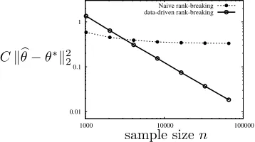
Figure 4: Data-driven rank-breaking is consistent, while a random rank-breaking results in incon-sistency.
generally inconsistent. However, when sample size is small, inconsistent estimators can achieve smaller variance leading to smaller error. Normalization constant C is 103`/d2, and each point is
averaged over 100 trials. We use the minorization-maximization algorithm from Hunter (2004) for computing the estimates from the rank-breakings.
Even if we use the consistent rank-breakings first proposed in Azari Soufiani et al. (2014), there is ambiguity in the choice of the weights. We next study how much we gain by using the proposed optimal choice of the weights. The optimal choice,λj,a = 1/(κj−pj,a), depends on two parameters: the size of the offeringsκj and the position of the separatorspj,a. To distinguish the effect of these two parameters, we first experiment with fixedκj =κ and illustrate the gain of the optimal choice
of λj,a’s.
0.01 0.1 1 10
2 10 100
consistent rank-breaking with uniform weights data-driven rank-breaking
Top-1 and bottom-(`−1) separators
Ckbθ−θ∗k2
2
number of separators `
4 5
6 7
8 9
10
1 2
3
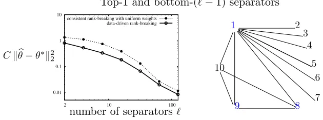
Figure 5: There is a constant factor gain of choosing optimal λj,a’s when the size of offerings are fixed, i.e. κj =κ(left). We choose a particular set of separators where one separators is at position
one and the rest are at the bottom. An example for`= 3 andκ= 10 is shown, where the separators are indicated by blue (right).
Figure 5 illustrates that the optimal choice of the weights improves over consistent rank-breaking with uniform weights by a constant factor. We fix κ = 128 and n = 128000. As illustrated by a figure on the right, the position of the separators are chosen such that there is one separator at position one, and the rest of`−1 separators are at the bottom. Precisely, (pj,1, pj,2, pj,3, . . . , pj,`) =
(1,128−`+ 1,128−`+ 2, . . . ,127). We consider this scenario to emphasize the gain of optimal weights. Observe that the MSE does not decrease at a rate of 1/` in this case. The parameter γ
which appears in the bound of Theorem 2 is very small when the breaking positionspj,a are of the
order κj as is the case here, when` is small. Normalization constantC isn/d2.
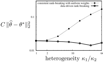
The gain of optimal weights is significant when the size ofSj’s are highly heterogeneous. Figure 6 compares performance of the proposed algorithm, for the optimal choice and uniform choice of weights λj,a when the comparison sets Sj’s are of different sizes. We consider the case when n1
agents provide their top-`1 choices over the sets of sizeκ1, andn2 agents provide their top-1 choice over the sets of size κ2. We take n1 = 1024, `1 = 8, and n2 = 10n1`1. Figure 6 shows MSE for the two choice of weights, when we fix κ1 = 128, and vary κ2 from 2 to 128. As predicted
from our bounds, when optimal choice of λj,a is used MSE is not sensitive to sample set sizes
κ2. The error decays at the rate proportional to the inverse of the effective sample size, which is
n1`1+n2`2 = 11n1`1. However, with λj,a = 1 when κ2 = 2, the MSE is roughly 10 times worse.
0.01 0.1
2 64
1 10
consistent rank-breaking with uniform weights data-driven rank-breaking
Ckbθ−θ∗k2
2
heterogeneityκ1/κ2
Figure 6: The gain of choosing optimalλj,a’s is significant whenκj’s are highly heterogeneous.
from small set size do not contribute without proper normalization. This gap in MSE corroborates bounds of Theorem 8. Normalization constant C is 103/d2.
4. The Role of the Topology of the Data
We study the role of topology of the data that provides a guideline for designing the collection of data when we do have some control, as in recommendation systems, designing surveys, and crowdsourcing. The core optimization problem of interest to the designer of such a system is to achieve the best accuracy while minimizing the number of questions.
4.1 The Role of the Graph Laplacian
Using the same number of samples, comparison graphs with larger spectral gap achieve better accuracy, compared to those with smaller spectral gaps. To illustrate how graph topology effects the accuracy, we reproduce known spectral properties of canonical graphs, and numerically compare the performance of data-driven rank-breaking for several graph topologies. We follow the examples and experimental setup from Shah et al. (2015a) for a similar result with pairwise comparisons. Spectral properties of graphs have been a topic of wide interest for decades. We consider a scenario where we fix the size of offerings as κj =κ =O(1) and each agent provides partial ranking with ` separators, positions of which are chosen uniformly at random. The resulting spectral gapα of different choices of the set Sj’s are provided below. The total number edges in the comparisons
graph (counting hyper-edges as multiple edges) is defined as|E| ≡ κ2 n.
• Complete graph: when |E| is larger than d2
, we can design the comparison graph to be a complete graph over d nodes. The weight Aii0 on each edge is n `/(d(d−1)), which is the
effective number of samples divided by twice the number of edges. Resulting spectral gap is one, which is the maximum possible value. Hence, complete graph is optimal for rank aggregation.
• Chain graph: we consider a chain of sets of sizeκ overlapping only by one item. For example,
S1 = {1, . . . , κ} and S2 = {κ, κ + 1, . . . ,2κ −1}, etc. We choose n to be a multiple of τ ≡ (d−1)/(κ−1) and offer each set n/τ times. The resulting graph is a chain of size κ
cliques, and standard spectral analysis shows that α = Θ(1/d2). Hence, a chain graph is strictly sub-optimal for rank aggregation.
• Star-like graph: We choose one item to be the center, and every offer set consists of this center node and a set ofκ−1 other nodes chosen uniformly at random without replacement. For example, center node ={1},S1 ={1,2, . . . , κ} andS2 ={1, κ+ 1, κ+ 2, . . . ,2κ−1}, etc.
nis chosen in the way similar to that of the Chain graph. Standard spectral analysis shows thatα= Θ(1) and star-like graphs are near-optimal for rank-aggregation.
• Barbell-like graph: We select an offering S = {S0, i, j}, |S0| = κ−2 uniformly at random and divide rest of the items into two groups V1 andV2. We offer setS nκ/d times. For each
offering of setS, we offerd/κ−1 sets chosen uniformly at random from the two groups{V1, i}
and{V2, j}. The resulting graph is a barbell-like graph, and standard spectral analysis shows thatα= Θ(1/d2). Hence, a chain graph is strictly sub-optimal for rank aggregation.
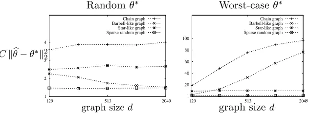
Figure 7 illustrates how graph topology effects the accuracy. When θ∗ is chosen uniformly at random, the accuracy does not change with d (left), and the accuracy is better for those graphs with larger spectral gap. However, for a certain worst-case θ∗, the error increases with dfor the chain graph and the barbell-like graph, as predicted by the above analysis of the spectral gap. We use`= 4,κ= 17 and vary dfrom 129 to 2049. κ is kept small to make the resulting graphs more like the above discussed graphs. Figure on left shows accuracy whenθ∗ is chosen i.i.d. uniformly over [−b, b] withb= 2. Error in this case is roughly same for each of the graph topologies with chain graph being the worst. However, when θ∗ is chosen carefully error for chain graph and barbell-like graph increases with d as shown in the figure right. We chose θ∗ such that all the items of a set have same weight, eitherθi= 0 or θi =bfor chain graph and barbell-like graph. We divide all the sets equally between the two types for chain graph. For barbell-like graph, we keep the two types of sets on the two different sides of the connector set and equally divide items of the connector set into two types. Number of samples n is 100(d−1)/(κ−1) and each point is averaged over 100 instances. Normalization constantC isn`/d2.
1 2 3 4
129 513 2049 Chain graph Barbell-like graph Star-like graph Sparse random graph
Ckθb−θ∗k22
graph sized
Randomθ∗
1 20 40 60 80 100
129 513 2049
Chain graph Barbell-like graph Star-like graph Sparse random graph
graph sized
Worst-caseθ∗
4.2 The Role of the Position of the Separators
As predicted by theorem 2, rank-breaking fails whenγ is small, i.e. the position of the separators are very close to the bottom. An extreme example is the bottom-`separators scenario, where each person is offered κ randomly chosen alternatives, and is asked to give a ranked list of bottom `
alternatives. In other words, the ` separators are placed at (pj,1, . . . , pj,`) = (κj −`, . . . , κ−1).
In this case, γ ' 0 and the error bound is large. This is not a weakness of the analysis. In fact we observe large errors under this scenario. The reason is that many alternatives that have large weightsθi’s will rarely be even compared once, making any reasonable estimation infeasible.
Figure 8 illustrates this scenario. We choose `= 8, κ = 128, andd= 1024. The other settings are same as that of the first figure of Figure 2. The left figure plots the magnitude of the estimation error for each item. For about 200 strong items among 1024, we do not even get a single comparison, hence we omit any estimation error. It clearly shows the trend: we get good estimates for about 400 items in the bottom, and we get large errors for the rest. Consequently, even if we only take those items that have at least one comparison into account, we still get large errors. This is shown in the figure right. The error barely decays with the sample size. However, if we focus on the error for the bottom 400 items, we get good error rate decaying inversely with the sample size. Normalization constantC in the second figure is 102x d/`and 102(400)d/`for the first and second
lines respectively, wherexis the number of items that appeared in rank-breaking at least once. We solve convex program (3) for θ restricted to the items that appear in rank-breaking at least once. The second figure of Figure 8 is averaged over 1000 instances.
0.1 1 10
200 400 600 800 1000
|bθi−θi∗|
Bottom-8 separators
item number
Weak Strong
0.001 0.01 0.1 1
10000 100000 items appearing in rank-breaking at least once
weakest 400 items
Ckbθe−θe∗k2 2
sample size n
Figure 8: Under the bottom-` separators scenario, accuracy is good only for the bottom 400 items (left). As predicted by Theorem 7, the mean squared error on the bottom 400 items scale as 1/n, where as the overall mean squared error does not decay (right).
We make this observation precise in the following theorem. Applying rank-breaking to only to those weakest deitems, we prove an upper bound on the achieved error rate that depends
on the choice of the de. Without loss of generality, we suppose the items are sorted such that θ∗1 ≤θ∗2 ≤ · · · ≤ θd∗. For a choice of de=`d/(2κ), we denote the weakest deitems byθe∗ ∈Rdesuch
that θei∗ =θi∗−(1/de) Pde
i0=1θi∗0, fori∈[de]. Since θ∗ ∈Ωb,θe∗ ∈[−2b,2b]de. The space of all possible
preference vectors for [de] items is given byΩ =e {θe∈Rde: Pde
i=1θie = 0} andΩe2b=Ωe∩[−2b,2b]de.
Although the analysis can be easily generalized, to simplify notations, we fixκj =κand `j =`
ditems for all j∈[n]. The rank-breaking log likelihood function LRB(θe) for the set of items [de] is
given by
LRB(θe) = n X
j=1 `j
X
a=1 λj,a
n X
(i,i0)∈E
j,a
I
i,i0∈[d]e
θi0−log
eθi+eθi0
o
. (17)
We analyze the rank-breaking estimator
b e
θ ≡ max
e
θ∈Ωe2b
LRB(eθ). (18)
We further simplify notations by fixingλj,a = 1, since from Equation (24), we know that the error increases by at most a factor of 4 due to this sub-optimal choice of the weights, under the special scenario studied in this theorem.
Theorem 7. Under the bottom-`separators scenario and the PL model,Sj’s are chosen uniformly at random of size κ andnpartial orderings are sampled overditems parametrized by θ∗∈Ωb. For
e
d=`d/(2κ) and any `≥4, if the effective sample size is large enough such that
n` ≥
214e8b χ2
κ3 `3
dlogd , (19)
where
χ ≡ 1
4 1−exp
− 2
9(κ−2)
!
, (20)
then the rank-breaking estimator in (18) achieves
1
p e d
bθe−θe∗
2 ≤
128(1 +e4b)2 χ
κ3/2 `3/2
r dlogd
n` , (21)
with probability at least 1−3e3d−3.
Consider a scenario where κ = O(1) and ` = Θ(κ). Then, χ is a strictly positive constant, and also κ/` is s finite constant. It follows that rank-breaking requires the effective sample size
n`=O(dlogd/ε2) in order to achieve arbitrarily small error of ε >0, on the weakest de=` d/(2κ)
items.
5. Real-World Data Sets
To validate our approach, we first take the estimated PL weights of the 10 types of sushi, using Hunter (2004) implementation of the ML estimator, over the entire input data of 5000 complete rankings. We take thus created output as the ground truth θ∗. To create partial rankings and compare the performance of the data-driven rank-breaking to the state-of-the-art GMM approach in Figure 9, we first fix ` = 6 and vary n to simulate top-`-separators scenario by removing the known ordering among bottom 10−`alternatives for each sample in the data set (left). We next fix n = 1000 and vary ` and simulate top-`-separators scenarios (right). Each point is averaged over 1000 instances. The mean squared error is plotted for both algorithms.
0.1 1
500 1000 2000 3000 4000 5000
data-driven rank-breaking GMM
kbθ−θ∗k2 2
sample sizen
Top-6 separators
0.01 0.1 1 10
1 2 3 4 5 6 7 8 9 data-driven rank-breaking
GMM Top-` separators
number of separators`
Figure 9: The data-driven rank-breaking achieves smaller error compared to the state-of-the-art GMM approach.
Figure 10 illustrates the Kendall rank correlation of the rankings estimated by the two algo-rithms and the ground truth. Larger value indicates that the estimate is closer to the ground truth, and the data-driven rank-breaking outperforms the state-of-the-art GMM approach.
0.8 0.84 0.88
500 1000 2000 3000 4000 5000 data-driven rank-breaking
GMM
Top-6 separators
Kendall Correlation
sample sizen
0.3 0.4 0.5 0.6 0.7 0.8 0.9 1
1 2 3 4 5 6 7 8 9 data-driven rank-breaking
GMM Top-` separators
number of separators`
Figure 10: The data-driven rank-breaking achieves larger Kendall rank correlation compared to the state-of-the-art GMM approach.
To validate whether PL model is the right model to explain the sushi data set, we compare the data-driven rank-breaking, MLE for the PL model, GMM for the PL model, Borda count and Spearman’s footrule optimal aggregation. We measure the Kendall rank correlation between the estimates and the samples and show the result in Table 1. In particular, if σ1, σ2,· · ·, σn denote sample rankings andσbdenote the aggregated ranking then the correlation value is (1/n)Pn
i=1 1− 4K(bσ,σi)
κ(κ−1)
for different number of samples n and different values of ` under the top-` separators scenarios. When `= 9, we are using all the complete rankings, and all algorithms are efficient. When` <9, we have partial orderings, and Spearman’s footrule optimal aggregation is NP-hard. We instead use scaled footrule aggregation (SFO) given in Dwork et al. (2001). Most approaches achieve similar performance, except for the Spearman’s footrule. The proposed data-driven rank-breaking achieves a slightly worse correlation compared to other approaches. However, note that none of the algorithms are necessarily maximizing the Kendall correlation, and are not expected to be particularly good in this metric.
MLE under PL
data-driven
RB GMM
Borda count
Spearman’s footrule
n= 500, `= 9 0.306 0.291 0.315 0.315 0.159
n= 5000,
`= 9 0.309 0.309 0.315 0.315 0.079
n= 5000,
`= 2 0.199 0.199 0.201 0.200 0.113
n= 5000,
`= 5 0.217 0.200 0.217 0.295 0.152
Table 1: Kendall rank correlation on sushi data set.
We compare our algorithm with the GMM algorithm on two other real-world data-sets as well. We use jester data set (Goldberg et al., 2001) that consists of over 4.1 million continuous ratings between−10 to +10 of 100 jokes from 48,483 users. The average number of jokes rated by an user is 72.6 with minimum and maximum being 36 and 100 respectively. We convert continuous ratings into ordinal rankings. This data-set has been used by Miyahara and Pazzani (2000); Polat and Du (2005); Cortes et al. (2007); Lebanon and Mao (2007) for rank aggregation and collaborative filtering.
Similar to the settings of sushi data experiments, we take the estimated PL weights of the 100 jokes over all the rankings as ground truth. Figure 11 shows comparative performance of the data-driven rank-breaking and the GMM for the two scenarios. We first fix `= 10 and vary nto simulate random-10 separators scenario (left). We next take all the rankings n= 73421 and vary
`to simulate random-`separators scenario (rights). Since sets have different sizes, while varying `
we use full breaking if the setsize is smaller than`. Each point is averaged over 100 instances. The mean squared error is plotted for both algorithms.
1 2 3
8000 24000 48483 data-driven rank-breaking
GMM
kθb−θ∗k22
sample sizen
Random-10 separators
0.01 0.1 1 10
1 20 40 60 80 99 data-driven rank-breaking
GMM Random-`separators
number of separators`
Figure 11: jester data set: The data-driven rank-breaking achieves smaller error compared to the state-of-the-art GMM approach.
0.001 0.01 0.1
5738 1000 2000 3000 4000 5000
data-driven rank-breaking GMM
kθb−θ∗k22
sample sizen
Random-3 separators
0.001 0.01 0.1
1 2 3 4
data-driven rank-breaking GMM
Random-`separators
number of separators`
Figure 12: APA data set: The data-driven rank-breaking achieves smaller error compared to the state-of-the-art GMM approach.
6. Related Work
and Suh (2015) proposed a new algorithm based on Rank Centrality that provides a tighter error bound for L∞ norm, as opposed to the existing L2 error bounds. Another interesting direction
in learning to rank is non-parametric learning from paired comparisons, initiated in several recent papers such as Duchi et al. (2010); Rajkumar and Agarwal (2014); Shah et al. (2015b); Shah and Wainwright (2015).
More recently, a more general problem of learning personal preferences from ordinal data has been studied (Yi et al., 2013; Lu and Boutilier, 2011b; Ding et al., 2015). The MNL model provides a natural generalization of the PL model to this problem. When users are classified into a small number of groups with same preferences, mixed MNL model can be learned from data as studied in Ammar et al. (2014); Oh and Shah (2014); Wu et al. (2015). A more general scenario is when each user has his/her individual preferences, but inherently represented by a lower dimensional feature. This problem was first posed as an inference problem in Lu and Negahban (2014) where convex relaxation of nuclear norm minimization was proposed with provably optimal guarantees. This was later generalized to k-way comparisons in Oh et al. (2015). A similar approach was studied with a different guarantees and assumptions in Park et al. (2015). Our algorithm and ideas of rank-breaking can be directly applied to this collaborative ranking under MNL, with the same guarantees for consistency in the asymptotic regime where sample size grows to infinity. However, the analysis techniques for MNL rely on stronger assumptions on how the data is collected, and especially on the independence of the samples. It is not immediate how the analysis techniques developed in this paper can be applied to learn MNL.
In an orthogonal direction, new discrete choice models with sparse structures has been proposed recently in Farias et al. (2009) and optimization algorithms for revenue management has been proposed Farias et al. (2013). In a similar direction, new discrete choice models based on Markov chains has been introduced in Blanchet et al. (2013), and corresponding revenue management algorithms has been studied in Feldman and Topaloglu (2014). However, typically these models are analyzed in the asymptotic regime with infinite samples, with the exception of Ammar and Shah (2011). A non-parametric choice models for pairwise comparisons also have been studied in Rajkumar and Agarwal (2014); Shah et al. (2015b). This provides an interesting opportunities to studying learning to rank for these new choice models.
We consider a fixed design setting, where inference is separate from data collection. There is a parallel line of research which focuses on adaptive ranking, mainly based on pairwise compar-isons. When performing sorting from noisy pairwise comparisons, Braverman and Mossel (2009) proposed efficient approaches and provided performance guarantees. Following this work, there has been recent advances in adaptive ranking Ailon (2011); Jamieson and Nowak (2011); Maystre and Grossglauser (2015b).
7. Discussion
weights in the estimator to achieve optimal performance, and also explicitly shows how the accuracy depends on the topology of the data.
This paper provides the first analytical result in the sample complexity of rank-breaking esti-mators, and quantifies the price we pay in accuracy for the computational gain. In general, more complex higher-order rank-breaking can also be considered, where instead of breaking a partial ordering into a collection of paired comparisons, we break it into a collection of higher-order com-parisons. The resulting higher-order rank-breakings will enable us to traverse the whole spectrum of computational complexity between the pairwise rank-breaking and the MLE. We believe this paper opens an interesting new direction towards understanding the whole spectrum of such ap-proaches. However, analyzing the Hessian of the corresponding objective function is significantly more involved and requires new technical innovations.
8. Proofs
8.1 Proof of Theorem 2
We prove a more general result for an arbitrary choice of the parameter λj,a > 0 for all j ∈ [n]
anda∈[`j]. The following theorem proves the (near)-optimality of the choice ofλj,a’s proposed in (10), and implies the corresponding error bound as a corollary.
Theorem 8. Under the hypotheses of Theorem 2 and any λj,a’s, the rank-breaking estimator achieves
1
√
d bθ−θ∗
2 ≤
4√2e4b(1 +e2b)2√dlogd α γ
q Pn
j=1 P`j
a=1 λj,a 2
κj−pj,a
κj −pj,a+ 1
Pn j=1
P`j
a=1λj,a(κj −pj,a)
,
(22)
with probability at least 1−3e3d−3, if n
X
j=1 `j
X
a=1
λj,a(κj−pj,a) ≥ 26e18b ηδ
α2βγ2τdlogd , (23) where γ,η, τ, δ, α, β, are now functions of λj,a’s and defined in (7), (8), (25), (27) and (30).
We first claim thatλj,a = 1/(κj−pj,a+ 1) is the optimal choice for minimizing the above upper bound on the error. From Cauchy-Schwartz inequality and the fact that all terms are non-negative, we have that
q Pn
j=1 P`j
a=1 λj,a 2
(κj−pj,a)(κj−pj,a+ 1)
Pn j=1
P`j
a=1λj,a(κj−pj,a)
≥ q 1
Pn j=1
P`j a=1
(κj−pj,a) (κj−pj,a+1)
, (24)
where λj,a = 1/(κj −pj,a + 1) achieves the universal lower bound on the right-hand side with an equality. Since Pn
j=1 P`j
a=1
(κj−pj,a) (κj−pj,a+1) ≥
Pn
j=1`j, substituting this into (22) gives the desired
error bound in (11). Although we have identified the optimal choice ofλj,a’s, we choose a slightly different value ofλ= 1/(κj−pj,a) for the analysis. This achieves the same desired error bound in
We first define all the parameters in the above theorem for general λj,a. With a slight abuse
of notations, we use the same notations forH, L,α and β for both the general λj,a’s and also the
specific choice of λj,a = 1/(κj −pj,a). It should be clear from the context what we mean in each case. Define
τ ≡ min
j∈[n]τj , where τj
≡
P`j
a=1λj,a(κj−pj,a)
`j (25)
δj,1 ≡
max
a∈[`j]
n
λj,a(κj−pj,a) o
+
`j
X
a=1 λj,a
, and δj,2≡ `j
X
a=1
λj,a (26)
δ ≡ max
j∈[n]
4δj,12 + 2 δj,1δj,2+δ
2 j,2
κj
ηj`j
. (27)
Note thatδ≥δ2j,1≥maxaλ2j,a(κj−pj,a)2≥τ2, and for the choice ofλj,a = 1/(κj−pj,a) it simplifies
asτ =τj = 1. We next define a comparison graphH for generalλj,a, which recovers the proposed
comparison graph for the optimal choice ofλj,a’s
Definition 9. (Comparison graph H). Each item i∈ [d] corresponds to a vertex i. For any pair of vertices i, i0, there is a weighted edge between them if there exists a set Sj such that i, i0 ∈Sj; the weight equals P
j:i,i0∈S
j τj`j κj(κj−1).
Let Adenote the weighted adjacency matrix, and let D= diag(A1). Define,
Dmax ≡ max
i∈[d]Dii = maxi∈[d]
X
j:i∈Sj τj`j
κj
≥ τminmax
i∈[d]
X
j:i∈Sj `j κj
. (28)
Define graph Laplacian Las L=D−A, i.e.,
L =
n X
j=1
τj`j κj(κj−1)
X
i<i0∈S
j
(ei−ei0)(ei−ei0)>. (29)
Let 0 = λ1(L) ≤ λ2(L) ≤ · · · ≤ λd(L) denote the sorted eigenvalues of L. Note that Tr(L) =
Pd i=1
P
j:i∈Sjτj`j/κj =
Pn
j=1τj`j. Defineα and β such that
α≡ λ2(L)(d−1)
Tr(L) =
λ2(L)(d−1) Pn
j=1τj`j
and β≡ Tr(L)
dDmax
=
Pn j=1τj`j dDmax
. (30)
For the proposed choice of λj,a = 1/(κj −pj,a), we have τj = 1 and the definitions of H, L, α, and β reduce to those defined in Definition 1. We are left to prove an upper bound, δ ≤
32(log(`max+ 2))2, which implies the sufficient condition in (9) and finishes the proof of Theorem
2. We have,
δj,1= max
a∈[`j]
n
λj,a(κj−pj,a)o+
`j
X
a=1
λj,a = 1 +
`j
X
a=1
1
κj−pj,a
≤ 1 +
`j
X
a=1
1
a
where in the first inequality follows from taking the worst case for the positions, i.e. pj,a = κj−`j+a−1 Using the fact that for any integerx,P`a=0−11/(x+a)≤log((x+`−1)/(x−1)), we
also have
δj,2κj ηj`j
≤
`j
X
a=1
1
κj−pj,a
max{`j, κj−pj,`j} `j
≤ minnlog(`j + 2),logκj−pj,`j+`j−1 κj−pj,`j −1
omax{`j, κj −pj,`
j} `j
≤ log(`j+ 2)`j
max{`j, κj−pj,`j−1}
max{`j, κj−pj,`j} `j
≤ 2 log(`j+ 2), (32)
where the first inequality follows from the definition of ηj, Equation (8). From (31), (32), and the fact that δj,2≤log(`j+ 2), we have
δ = max
j∈[n]
4δj,12 + 2 δj,1δj,2+δ
2 j,2
κj ηj`j
≤ 28(log(`max+ 2))2.
8.2 Proof of Theorem 8
We first introduce two key technical lemmas. In the following lemma we show thatEθ∗[∇LRB(θ∗)] =
0 and provide a bound on the deviation of∇LRB(θ∗) from its mean. The expectationEθ∗[·] is with
respect to the randomness in the samples drawn according toθ∗. The log likelihood Equation (2) can be rewritten as
LRB(θ) =
n X j=1 `j X a=1 X
i<i0∈S
j
I
(i,i0)∈G
j,a λj,a
θiI
σ−1j (i)<σ−1j (i0) +θi0Iσ−1
j (i)>σ
−1
j (i0)
−logeθi+eθi0
.
(33)
We use (i, i0) ∈ Gj,a to mean either (i, i0) or (i0, i) belong to Ej,a. Taking the first-order partial derivative of LRB(θ), we get
∇iLRB(θ∗) = X
j:i∈Sj `j
X
a=1 X
i0∈S
j i06=i
λj,aI (i,i0)∈G
j,a I
σ−1j (i)<σ−1j (i0) −
exp(θ∗i) exp(θi∗) + exp(θi∗0)
!
. (34)
Lemma 10. Under the hypotheses of Theorem 2, with probability at least 1−2e3d−3,
∇LRB(θ∗) 2 ≤ v u u u t6 logd
n X j=1 `j X a=1 λj,a 2
κj−pj,a
κj−pj,a+ 1
.
The Hessian matrix H(θ)∈ Sd withH
ii0(θ) = ∂ 2L
RB(θ)
∂θi∂θi0 is given by
H(θ) =−
n X j=1 `j X a=1 X
i<i0∈S
j
I
(i,i0)∈G
j,a λj,a (ei
−ei0)(ei−ei0)> exp(θi+θi 0)
[exp(θi) + exp(θi0)]2
!