Structure Learning in Bayesian Networks of a Moderate Size by Efficient Sampling

Structure Learning in Bayesian Networks of a Moderate Size by

Efficient Sampling

Ru He [email protected]

Department of Computer Science and Department of Statistics Iowa State University

Ames, IA 50011, USA

Jin Tian [email protected]

Department of Computer Science Iowa State University

Ames, IA 50011, USA

Huaiqing Wu [email protected]

Department of Statistics Iowa State University Ames, IA 50011, USA

Editor:Max Chickering

Abstract

We study the Bayesian model averaging approach to learning Bayesian network structures (DAGs) from data. We develop new algorithms including the first algorithm that is able to efficiently sample DAGs of a moderate size (with up to about 25 variables) according to the exact structure posterior. The DAG samples can then be used to construct estimators for the posterior of any feature. We theoretically prove good properties of our estimators and empirically show that our estimators con-siderably outperform the estimators from the previous state-of-the-art methods.

Keywords: Bayesian model averaging, Bayesian networks, DAG sampling, dynamic

program-ming, order sampling, structure learning

1. Introduction

Bayesian networks are graphical representations of multivariate joint probability distributions and have been widely used in various data-mining tasks for probabilistic inference and causal model-ing (Pearl, 2000; Spirtes et al., 2001). The core of a Bayesian network (BN) representation is its Bayesian network structure. A Bayesian network structure is a DAG (directed acyclic graph) whose nodes represent the random variables X1, X2,· · ·, Xn in the problem domain and whose edges

correspond to the direct probabilistic dependencies. Semantically, a Bayesian network structureG encodes a set of conditional independence assumptions: for each variable (node)Xi,Xiis

In the last two decades, there have been a large number of research articles focusing on the problem of learning Bayesian network structure(s) from the data. These articles deal with a common real situation where the underlying Bayesian network is typically unknown so that it has to be learned from the observed data. One motivation for the structure learning is to use the learned structure for inference or decision making. For example, we can use the learned model to predict or classify a new instance of data. Another structure-learning motivation, which is more closely related to the semantics of Bayesian network structures, is for discovering the structure of the problem domain. For example, in the context of biological expression data, the discovery of the causal and dependence relation among different genes is often of primary interests. With the semantics of a Bayesian network structure G, the existence of an edge from node X to node Y inG can be interpreted as the fact that variableXdirectly influences variableY; the existence of a directed path from nodeXto nodeY can be interpreted as the fact thatXeventually influencesY. Furthermore, under certain assumptions (Heckerman et al., 1999; Spirtes et al., 2001), the existence of a directed path from nodeX to nodeY indicates thatXcausesY. Thus, with the learned Bayesian network structure, we can answer interesting questions such as whether geneX controls geneY which in turn controls geneZby examining whether there is a directed path from nodeXvia nodeY to node Zin the learned structure. Just as mentioned by Friedman and Koller (2003), the extraction of these kinds of interesting structural features is often the primary goal in the discovery task.

There are several general approaches to learning BN structures. One approach is to treat learning BN structures as a model-selection problem. This approach defines a scoring criterion that measures how well a BN structure (DAG) fits the data and finds the DAG (or a set of equivalent DAGs) with the optimal score (Silander and Myllymaki, 2006; Jaakkola et al., 2010; Yuan et al., 2011; Malone et al., 2011a,b; Cussens, 2011; Yuan and Malone, 2012; Malone and Yuan, 2013; Cussens and Bartlett, 2013; Yuan and Malone, 2013). (In Bayesian approach, the score of a DAGGis simply the posterior p(G|D)ofGgiven dataD.) When the data size is small as compared with the number of variables, however, the posteriorp(G|D) often gives significant support to a number of DAGs, and using a single maximum-a-posteriori (MAP) model could lead to unwarranted conclusions (Friedman and Koller, 2003). It is therefore desirable to use the Bayesian model averaging approach by which the posterior probability of any feature of interest is computed by averaging over all the possible DAGs (Heckerman et al., 1999).

assump-tion, called the order-modular assumpassump-tion, will be discussed in details soon.) This DP algorithm has (even higher) exponential time and space complexity and can only handle a Bayesian network with fewer than20variables (mainly because of its space costO(3n)). Because this DP algorithm can only deal with a path feature, all the other non-modular features (such as a combined path) which would interest various users still cannot be computed by any DP algorithm proposed so far. Note that generally the posteriorp(f|D)of a combined featuref = (f1, f2, . . . , fJ)cannot be obtained

only from the posterior of each individual featurep(fj|D) (j ∈ {1,2, . . . , J}), because the

inde-pendence among these features does not hold generally. Actually, by comparingp(f2|f1, D)with p(f2|D), a user can know the effect of the featuref1upon the featuref2; but to obtainp(f2|f1, D) (=p(f1, f2|D)/p(f1|D)), the user typically needs to obtainp(f1, f2|D)first. Another limitation of all these DP algorithms is that it is very expensive for them to perform data prediction tasks. They can compute the exact posterior of a new observational data casep(x|D)but the algorithms have to be re-run for each new data casex.

One solution to computing the posterior of an arbitrary non-modular feature is drawing DAG samples {G1, . . . , GT} from the posterior p(G|D), which can then be used to approximate the

full Bayesian model averaging by estimating the posterior of an arbitrary feature f as p(f|D)

≈ 1

T

PT

i=1f(Gi), or the posterior predictive distribution asp(x|D)≈ _T1 PTi=1p(x|Gi). A number

of algorithms have been developed for drawing sample DAGs using the bootstrap technique (Fried-man et al., 1999) or the Markov chain Monte Carlo (MCMC) techniques (Madigan and York, 1995; Friedman and Koller, 2003; Eaton and Murphy, 2007; Grzegorczyk and Husmeier, 2008; Niinimaki et al., 2011; Niinimaki and Koivisto, 2013). Madigan and York (1995) developed the Structure MCMC algorithm that uses the Metropolis-Hastings algorithm in the space of DAGs. Friedman and Koller (2003) developed theOrder MCMCprocedure that operates in the space of orders. The Order MCMC was shown to be able to considerably improve over the Structure MCMC the mix-ing and convergence of the Markov chain and to outperform the bootstrap approach of Friedman et al. (1999) as well. Eaton and Murphy (2007) developed the Hybrid MCMC method (that is, DP+MCMC method) that first runs the DP algorithm of Koivisto (2006) to develop a global pro-posal distribution and then runs the MCMC phase in the DAG space. Their experiments showed that the Hybrid MCMC converged faster than both the Structure MCMC and the Order MCMC, so that the Hybrid MCMC resulted in more accurate structure-learning performance. An improved MCMC algorithm (often denoted asREV-MCMC) traversing in the DAG space with the addition of a new edge-reversal move was developed by Grzegorczyk and Husmeier (2008) and was shown to be superior to the Structure MCMC and nearly as efficient as the Order MCMC in the mixing and convergence. Recently, Niinimaki et al. (2011) proposed thePartial Order MCMCmethod which operates in the space of partial orders. The Partial Order MCMC includes the Order MCMC as its special case (by setting the parameter bucket sizebto be 1) and has been shown to be superior to the Order MCMC in terms of the mixing and the structure-learning performance when a more appro-priate bucket sizeb >1is set. One common drawback of these MCMC algorithms is that there is no guarantee on the quality of the approximation in finite runs. The approach to approximating the full Bayesian model averaging using theK-bestBayesian network structures was studied by Tian et al. (2010) and was shown to be competitive with the Hybrid MCMC.

order-modular prior (Friedman and Koller, 2003; Koivisto and Sood, 2004), for computational conve-nience. (Please refer to the beginning of Section 2.1 for the definition of the order-modular prior.) Under the assumption of the order-modular prior, however, the corresponding prior p(G) cannot represent some desirable priors such as a uniform prior over the DAG space1; the computed pos-terior probabilities are biased because a DAG that has a larger number of topological orders will be assigned a larger prior probability. Whether a computed posterior with the bias from the order-modular prior is inferior to its counterpart without such a bias depends on the application scenario and is beyond the scope of this paper. For the detailed discussion about this issue, please see the related papers (Friedman and Koller, 2003; Grzegorczyk and Husmeier, 2008; Parviainen and Koivisto, 2011)2. One method that helps the Order MCMC (Friedman and Koller, 2003) to correct this bias was proposed by Ellis and Wong (2008).

In this paper, first we develop a new algorithm that uses the results of the DP algorithm of Koivisto and Sood (2004) to efficiently sample orders according to theexactorder posterior under the assumption of the order-modular prior. Next, we develop a time-saving strategy for the pro-cess of sampling DAGs consistent with given orders. (Such a DAG-sampling propro-cess is based on sampling parents for each node as described by Friedman and Koller, 2003 by assuming a bounded node in-degree.) The resulting algorithm (called DDS) is the first algorithm that is able to sample DAGs according to theexactDAG posterior with the same order-modular prior assumption. We em-pirically show that our DDS algorithm is both considerably more accurate and considerably more efficient than the Order MCMC and the Partial Order MCMC whennis moderate so that our DDS algorithm is applicable. Moreover, the estimator based on our DDS algorithm has several desirable properties; for example, unlike the existing MCMC algorithms, the quality of our estimator can be guaranteed by controlling the number of DAGs sampled by our DDS algorithm. The main appli-cation of our DDS algorithm is to address the limitation of the exact DP algorithms (Koivisto and Sood, 2004; Koivisto, 2006; Parviainen and Koivisto, 2011) (whose usage is restricted to modular features or path features) in order to estimate the posteriors of variousnon-modularfeatures arbi-trarily specified by users. Additionally our DDS algorithm can also be used to efficiently perform data prediction tasks in estimating p(x|D) for a large number of data cases (while the exact DP algorithm has to be re-run for each data casex). Finally, we develop an algorithm (called IW-DDS) to correct the bias (due to the order-modular prior) in the DDS algorithm by extending the idea of Ellis and Wong (2008). We theoretically prove that the estimator based on our IW-DDS has sev-eral desirable properties; then we empirically show that our estimator is superior to the estimators based on the Hybrid MCMC method (Eaton and Murphy, 2007) and the K-best algorithm (Tian et al., 2010), two state-of-the-art algorithms that can estimate the posterior of any feature without the order-modular prior assumption. Analogously, our IW-DDS algorithm mainly addresses the limitation of the exact DP algorithm of Tian and He (2009) (whose usage is restricted to modular features) in order to estimate the posteriors of arbitrarynon-modularfeatures and can additionally be used to efficiently perform data prediction tasks when an application situation prefers to avoid the bias from the order-modular prior.

1. A uniform prior over the DAG space can be represented in another form of the structure prior, termed as the

structure-modularprior. The definition of the structure-modular prior will be given in Eq. (2) in Section 2.

The rest of the paper is organized as follows. In Section 2 we briefly review the Bayesian approach to learning Bayesian networks from data, the related DP algorithms (Koivisto and Sood, 2004; Koivisto, 2006), and the Order MCMC algorithm (Friedman and Koller, 2003). In Section 3 we present our order sampling algorithm, DDS algorithm, and IW-DDS algorithm, and prove good properties of the estimators based on our algorithms. We empirically demonstrate the advantages of our algorithms in Section 4 and conclude the paper in Section 5. Finally, Appendix A provides the proofs of all the conclusions including the propositions, theorems, and corollary referenced in the paper.

2. Bayesian Learning of Bayesian Network Structures

A Bayesian network structure is a DAG G that provides the skeleton for compactly encoding a joint probability distribution over a setX = {X1, . . . , Xn} of random variables with each node

of the DAG representing a variable in X. For convenience we typically work on the index set V = {1, . . . , n} and represent a variable Xi by its indexi. We useXP ai ⊆ X to represent the parent set ofXi in a DAGGand useP ai ⊆ V to represent the corresponding index set. (A pair

(i, P ai)is often called a family.) Thus, a DAGGcan be represented as a vector(P a1, . . . , P an).

Assume that we are given a training data setD={x1, x2, . . . , xm}, where eachxiis a particular instantiation over the set of variablesX. We only consider situations where the data are complete, that is, every variable in X is assigned a value. In the Bayesian approach to learning Bayesian networks from the training dataD, we compute the posterior probability of a DAGGas

p(G|D) = p(D|G)p(G) p(D) =

p(D|G)p(G)

P

Gp(D|G)p(G)

.

Assuming global and local parameter independence, and parameter modularity, we can decompose p(D|G) into a product of local marginal likelihoods (often called local scores) as (Cooper and Herskovits, 1992; Heckerman et al., 1995)

p(D|G) =

n

Y

i=1

p(Xi|XP ai :D) :=

n

Y

i=1

scorei(P ai :D), (1)

where, with appropriate parameter priors,scorei(P ai : D) (the local score for a family(i, P ai))

has a closed-form solution. In this paper we will assume that these local scores can be computed efficiently from data. The standard assumption for the structure priorp(G)is thestructure-modular

prior (Friedman and Koller, 2003)

p(G) =

n

Y

i=1

pi(P ai), (2)

wherepiis some nonnegative function over the subsets ofV − {i}.

Combining Eq. (1) and Eq. (2), we have

p_⊀(G, D) =p(D|G)p_⊀(G) =

n

Y

i=1

Note that the subscript⊀is intentionally added by us to mean that each correspondingly marked

probability is the one obtained under the structure-modular prior instead of the order-modular prior. This is different from the probability obtained under the order-modular prior, which will be marked by the subscript≺for the distinction.

We can compute the posterior probability of any feature of interest by averaging over all the possible DAGs. For example, we are often interested in computing the posteriors of structural features. Letfbe a structural feature represented by an indicator function such thatf(G)is 1 if the feature is present inGand 0 otherwise. By the full Bayesian model averaging, we have the posterior off as

p(f|D) =X

G

f(G)p(G|D). (4)

Note thatp_⊀(f|D)will be obtained ifp(G|D)in Eq. (4) isp_⊀(G|D);p≺(f|D)will be obtained ifp(G|D)in Eq. (4) isp≺(G|D). This difference is the key to understanding the bias issue which will be described in details later.

Because directly summing over all the possible DAGs by brute force is generally infeasible for any problem withn >6using a contemporary computer, one approach to computing the posterior off is to draw DAG samples{G1, . . . , GT}from the posteriorp⊀(G|D)orp≺(G|D), which can then be used to estimate the posteriorp_⊀(f|D)orp≺(f|D)as

ˆ

p(f|D) = 1 T

T

X

i=1

f(Gi). (5)

2.1 The DP Algorithms

The DP algorithms (Koivisto and Sood, 2004; Koivisto, 2006) work in the order space rather than the DAG space. We define anorder≺of variables as a total order (a linear order) onV represented as a vector(U1, . . . , Un), whereUi is the set of predecessors ofiin the order≺. To be more clear

we may useU_i≺. We say that a DAGG= (P a1, . . . , P an)is consistent with an order(U1, . . . , Un),

denoted byG⊆≺, ifP ai⊆Uifor eachi. IfSis a subset ofV, we letL(S)denote the set of linear

orders onS. In the following we will largely follow the notation from Koivisto (2006).

The algorithms working in the order space assume theorder-modularprior defined as follows: ifGis consistent with≺, then

p(≺, G) =

n

Y

i=1

qi(Ui)ρi(P ai), (6)

where eachqiandρiis some function from the subsets ofV− {i}to the nonnegative real numbers.

(IfGis not consistent with≺, thenp(≺, G) = 0.) Amodular featureis defined as

f(G) =

n

Y

i=1

fi(P ai),

wherefi(P ai)is an indicator function returning a0/1value. For example, an edge featurej → i

can be represented by always settingfl(P al) = 1for eachl=6 iand by settingfi(P ai) = 1if and

With the order-modular prior, we are interested in the posteriorp≺(f|D) =p≺(f, D)/p≺(D). Note that p≺(f|D) can be obtained if the joint probability p≺(f, D) can be computed, because p≺(D) =p≺(f ≡1, D)wheref ≡1, meaning thatf always equals 1, can be easily achieved by setting eachfi(P ai)to be the constant 1. Koivisto and Sood (2004) showed that

p(f,≺, D) =

n

Y

i=1

αi(Ui≺), (7)

and

p≺(f, D) =X ≺

n

Y

i=1

αi(Ui≺), (8)

where the functionαiis defined for eachi∈V and eachS⊆V − {i}as

αi(S) =qi(S)

X

P ai⊆S

βi(P ai),

in which the functionβiis defined for eachi∈V and eachP ai⊆V − {i}as

βi(P ai) =fi(P ai)ρi(P ai)scorei(P ai :D).

Accordingly, the DP algorithm of Koivisto and Sood (2004) consists of the following three steps. The first step computesβi(P ai)for eachi∈V and eachP ai ⊆V − {i}. The time complexity of

this step isO(nk+1_{C(m))under the assumption of the maximum in-degreek, wherenis the number} of variables, andC(m)is the cost of computing a single local marginal likelihoodscorei(P ai :D)

formdata instances. The second step computesαi(S)for eachi∈V and eachS⊆V − {i}. With

the assumed maximum in-degreek, this step takesO(kn2n_{) time by using the truncated M¨obius}

transform technique (Koivisto and Sood, 2004), which was extended from the standard fast M¨obius transform algorithm (Kennes and Smets, 1991). The third step computesp≺(f, D)by defining the following function (called forward contribution) for eachS⊆V:

L(S) = X ≺∈L(S)

Y

i∈S

αi(Ui≺), (9)

whereU_i≺ is the set of variables inS ahead ofiin the order≺∈ L(S). It can be shown that for everyS ⊆V,L(S)can be computed recursively using the DP technique according to the following equation (Koivisto and Sood, 2004; Koivisto, 2006):

L(S) =X

i∈S

αi(S− {i})L(S− {i}), (10)

starting withL(∅) = 1and ending withL(V). From Eq. (8) and Eq. (9), we have

p≺(f, D) =L(V). (11)

As the extended work of Koivisto and Sood (2004), Koivisto (2006) included the DP algorithm of Koivisto and Sood (2004) as its first three steps and appended two additional steps so that all the n(n−1) edges can be computed in O(nk+1C(m) + kn2n) time and O(n2n) space. The foundation of the two additional steps is the introduction of the following function (called backward contribution) for eachT ⊆V:

R(T) = X ≺0_∈L(T)

Y

i∈T

αi((V −T)∪U≺

0

i ). (12)

Essentially, R(T) represents the contribution of the variables in T when they are the last|T| el-ements in the unknown linear order on V. Like L(S), R(T) can also be computed recursively using some DP technique. Please refer to the paper of Koivisto (2006) for further details of the two additional steps.

Although the DP algorithms (Koivisto and Sood, 2004; Koivisto, 2006) make significant contri-butions to the structure learning of Bayesian networks, they have one fundamental limitation: they can only compute the posteriors of modular features. In the next section, we will show how to use the results of the DP algorithm of Koivisto and Sood (2004) to efficiently draw DAG samples, which can then be used to compute the posteriors of arbitrary features.

2.2 Order MCMC

The idea of the Order MCMC is to use the Metropolis-Hastings algorithm to draw order samples

{≺₁, . . . ,≺_No}that havep(≺ |D)as the invariant distribution, whereNois the number of sampled

orders. For this purpose we need to be able to computep(≺, D), which can be obtained from Eq. (7) by settingf ≡1. Letβ0_i(P ai)denoteβi(P ai)resulted from setting eachfi(P ai)to be the constant

1. Similarly, we define α0_i(S) andL0(S) as the special cases ofαi(S) andL(S) by setting each

fi(P ai)to be the constant 1. Then from Eq. (7) and Eq. (11) we have

p(≺, D) =

n

Y

i=1

α_i0(U_i≺), (13)

and

p≺(D) =L0(V). (14)

The Order MCMC can estimate the posterior of a modular feature as

ˆ

p≺(f|D) = 1 No

No

X

i=1

p(f| ≺_i, D). (15)

For example, from Propositions 3.1 and 3.2 stated by Friedman and Koller (2003) as well as the definitions ofβ_i0andα0_i, the posterior of a particular choice of parent setP ai⊆U_i≺for nodeigiven

an order is

p((i, P ai)| ≺, D) =

β_i0(P ai)

α0_i(U_i≺)/qi(Ui≺)

and the posterior of the edge featurej →igiven an order is

p(j→i| ≺, D) = 1−α

0

i(Ui≺− {j})/qi(U

≺

i − {j})

α0_i(U_i≺)/qi(Ui≺)

. (17)

In order to compute arbitrary non-modular features, we further draw DAG samples after drawing No order samples. Given an order, a DAG can be sampled by drawing parents for each node

ac-cording to Eq. (16). Given DAG samples{G1, . . . , GT}, we can then estimate any feature posterior

p≺(f|D)usingp≺(fˆ |D)shown in Eq. (5).

3. Order Sampling Algorithm and DAG Sampling Algorithms

In this section we present our order sampling algorithm, DDS algorithm, and IW-DDS algorithm. We also prove good properties of the estimators based on our algorithms.

3.1 Order Sampling Algorithm

In this subsection, we show that using the results includingα0_i(S) (for eachi ∈ V and eachS ⊆

V − {i}) and L0(S) (for each S ⊆ V) computed from the DP algorithm of Koivisto and Sood (2004), we can draw an order sample efficiently by drawing each element in the order one by one. Let an order≺be represented as (σ1, . . . , σn), whereσiis theith element in the order.

Proposition 1 The conditional probability that the kth (1 ≤ k ≤ n) element in the order is σk

given that then−kelements after it along the order areσk+1, . . . , σnrespectively is as follows:

p(σk|σk+1, . . . , σn, D) =

L0(U_σ≺_k)α0_σk(U_σ≺_k) L0_(U≺

σk+1)

, (18)

whereσk∈V − {σk+1, . . . , σn}, andUσ≺i =V − {σi, σi+1, . . . , σn}so thatU ≺

σi denotes the set of

predecessors ofσiin the order≺.

Specifically fork=n, we essentially have

p(σn=i|D) =

L0(V − {i})α0_i(V − {i})

L0_(V) , (19)

wherei∈V.

Note that all the proofs in this paper are provided in Appendix A. It is clear that for each k∈ {1, . . . , n},P

i∈U_σk≺

+1p(σk =i

|σk+1, . . . , σn, D) = 1because of

Eq. (10) andU_σ≺_k = U_σ≺_k+1 − {σk}. Thus, p(σk|σk+1, . . . , σn, D) is a probability mass function

(pmf) withkpossibleσkvalues fromUσ≺k+1.

Based on Proposition 1, we propose the following order sampling algorithm to sample an order

≺:

• Sampleσn, the last element of the order≺, according to Eq. (19).

• For each kfrom n−1 down to 1: given the sampled (σk+1, . . . , σn), sampleσk, the kth

Provided that α0_i(S) (for eachi ∈ V and each S ⊆ V − {i}) andL0(S)(for each S ⊆ V) have been computed, sampling an order using the above algorithm takes onlyO(n2)time because sampling each elementσk(k∈ {1, . . . , n}) in the order takesO(n)time.

The following proposition guarantees the correctness of our order sampling algorithm.

Proposition 2 An order≺sampled according to our order sampling algorithm has its pmf equal to the exact posteriorp(≺ |D)under the order-modular prior, because

n

Y

k=1

p(σk|σk+1, . . . , σn, D) =p(≺ |D). (20)

The key to our order sampling algorithm is our realization that the results including α0_i(S) andL0(S)computed from the DP algorithm of Koivisto and Sood (2004) are already sufficient to guide the order sampling process. In an abstract point of view, the results computed from the DP algorithm of Koivisto and Sood (2004) are analogous to the answers provided by the #P-oracle stated in Theorem 3.3 of Jerrum et al. (1986). This theorem states that with the aid of a #P-oracle that is always able to provide the exact counting information (the exact number) of accept-ing configurations from a currently given configuration, a probabilistic Turaccept-ing machine can serve as a uniform generator so that every accepting configuration will be reached with an equal posi-tive probability. In our situation, instead of providing the exact counting information, the results computed from the DP algorithm of Koivisto and Sood (2004) are able to provide the exact joint probabilityp(σk, σk+1, . . . , σn, D) for a subsequence (σk, σk+1, . . . , σn) of any order ≺for any

k ∈ {1,2, . . . , n}, which is shown in the proof of Proposition 1 in Appendix A.1. As a result, the order sampling can be efficiently performed based on the definition of the conditional probability distribution.

3.2 DDS Algorithm

After drawing an order sample, we can then easily sample a DAG by drawing parents for each node according to Eq. (16) as described by Friedman and Koller (2003) (assuming a maximum in-degree k). This naturally leads to our algorithm, termed direct DAG sampling (DDS), as follows:

• Step 1: Run the DP algorithm of Koivisto and Sood (2004) with eachfi(P ai)set to be the

constant 1.

• Step 2 (Order sampling step): Sample No orders such that each order ≺ is independently

sampled according to our order sampling algorithm.

• Step 3 (DAG sampling step): For each sampled order≺, one DAG is independently sampled by drawing a parent set for each node of the DAG according to Eq. (16).

The correctness of our DDS algorithm is guaranteed by the following theorem.

Theorem 3 TheNo DAGs sampled according to the DDS algorithm are independent and

The time complexity of the DDS algorithm is as follows. Step 1 takesO(nk+1C(m) +kn2n) time (Koivisto and Sood, 2004), as discussed in Section 2.1. In Step 2, sampling each order takes O(n2)time. In Step 3, sampling each DAG takesO(nk+1)time. Thus, the overall time complexity of our DDS algorithm isO(nk+1C(m) +kn2n+n2No+nk+1No). Because typically we assume

k≥1, the order sampling process (Step 2) does not affect the overall time complexity of the DDS algorithm because of its efficiency.

The time complexity of our DDS algorithm depends on the assumption of the maximum in-degreek. Such an assumption is fairly innocuous, as discussed on page 101 of Friedman and Koller (2003), because DAGs with very large families tend to have low scores. (The maximum-in-degree assumption is also justified in the context of biological expression data on page 270 of Grzegorczyk and Husmeier, 2008.) Accordingly, this assumption has been widely used in the literature (Friedman and Koller, 2003; Koivisto and Sood, 2004; Ellis and Wong, 2008; Grzegorczyk and Husmeier, 2008; Niinimaki et al., 2011; Parviainen and Koivisto, 2011) and the maximum in-degree k has been set to be no greater than6in all of their experiments.

Note that the DAG sampling step of the DDS algorithm takes O(nk+1No) time. This will

dominate the overall running time of the DDS algorithm (even ifkis assumed to be3or4), when n is moderate (n ≤ 25) and the sample size No reaches several thousands. Therefore, for the

efficiency of our DDS algorithm, we have developed a time-saving strategy for the DAG sampling step, which will be described in details in Section 3.2.1.

Given DAG samples, p≺(fˆ |D), an estimator of the exact posterior of any arbitrary feature f, can be constructed by Eq. (5). LetCn,f denote the time cost of determining the structural feature

f in a DAG ofnnodes. Then constructingp≺(fˆ |D)takesO(Cn,fNo) time. (For example,Cn,fe =O(1)for an edge featurefe;Cn,fp=O(n

2_{)for a path featuref}

p.) If we only need order samples,

the algorithm consisting of Steps 1 and 2 will be called direct order sampling (DOS). Given order samples, for some modular featuref such as a parent-set feature or an edge feature,p(f| ≺_i, D) can be computed by Eq. (16) or (17), and then p≺(f|D) can be estimated by Eq. (15). (Because computing a parent-set feature or an edge feature by Eq. (16) or (17) takesO(1)time, estimating p≺(f|D)by Eq. (15) only takesO(No)time for these two features.)

As for the space cost of our DDS algorithm, note that Step 1 of our DDS takesO(n2n_)memory

space, which limits the application of our DDS to Bayesian networks with up to around 25 variables. Because a total order can be represented as a vector(U1, . . . , Un) and a DAG can be represented

as a vector (P a1, . . . , P an), both a total order and a DAG can be represented in O(n2) space

3_{. Therefore, Steps 2 and 3 of our DDS takeO(n}2_N

o) memory space, and the overall memory

requirement of our DDS algorithm isO(n2n+n2No).

Because of Theorem 3, the estimatorp≺(fˆ |D) based on our DDS algorithm has the following desirable properties.

Corollary 4 For any structural featuref, with respect to the exact posteriorp≺(f|D), the estimator

ˆ

p≺(f|D)based on theNo DAG samples from the DDS algorithm using Eq. (5) has the following

properties:

(i)p≺(fˆ |D)is an unbiased estimator ofp≺(f|D).

3. Whenn≤32, in the vector representation(P a1, . . . , P an)of a DAG, each parent setP aican be represented by

a 32-bit integer whosejth bit indicates whether or not nodeXjis a parent of nodeXi. Thus, a DAG of a moderate

sizencan be represented byn32-bit integers. Similarly, whenn≤32, in the vector representation(U1, . . . , Un)

of a total order, eachUican be represented by a 32-bit integer whosejth bit indicates whether or not nodeXjis a

(ii)p≺(fˆ |D)converges almost surely top≺(f|D). (iii) If0< p≺(f|D)<1, then the random variable

√

No(ˆp≺(f|D)−p≺(f|D))

p

ˆ

p≺(f|D)(1−p≺(fˆ |D))

has a limiting standard normal distribution.

(iv) For any > 0 and any 0 < δ < 1, if No ≥ (ln(2/δ))/(22), then P(|p≺(fˆ |D) −

p≺(f|D)|< )≥1−δ.

In particular, Corollary 4 (iv), which is essentially from the Hoeffding bound (Hoeffding, 1963; Koller and Friedman, 2009), ensures the probability that the error of the estimatorp≺(fˆ |D)from the DDS algorithm is bounded byto be at least1−δ, as long as the sample sizeNo≥(ln(2/δ))/(22).

This property, which the existing MCMC algorithms (Friedman and Koller, 2003; Niinimaki et al., 2011) do not have, can be used to obtain quality guarantee for the estimator from our DDS algorithm.

3.2.1 TIME-SAVINGSTRATEGY FOR THE DAG SAMPLING STEP OF THE DDS

The running time of the DAG sampling step (Step 3) of the DDS algorithm isO(nk+1No), which

will dominate the overall running time of the DDS algorithm whennis moderate and the sample size Noreaches several thousands. Thus, in this sub-subsection we introduce our strategy for effectively

reducing the running time of the DAG sampling step so that the efficiency of the overall DDS algorithm can be achieved.

In the DAG sampling step, each sampled order ≺i = (σ1, . . . , σn)≺i (1 ≤ i ≤ No) can be

represented as{(σ1, Uσ1)

≺i_{, . . . ,(σ}

n, Uσn)

≺i_{}, whereU}

σj denotes the set of predecessors ofσj in the order. For each sampled order≺_i, for each(σj, Uσj)

≺i _{(1 ≤ j ≤ n), we need to sample one} P aσj ofσj (one parent set ofσj) from a list{P aσjz}

σj

z including every parent setP aσjz ⊆ U ≺i

σj. LetZjbe the length of such a list. BecauseZj =P_imin₌₀{k,j−1} j−_i1

=O(nk), sampling oneP aσj forσjtakesO(nk)time and sampling one DAG takesO(nk+1)time. Note thatZj is an increasing

function ofjbut in the following we will use the notationZinstead ofZjfor notational convenience

when the context is clear. In the following we also will not use the plural for mathematical symbols to avoid notational confusion by ending “s”. The reader should assume the correct singular or plural case when reading.

WhenNo > 1, the overall running time of the DAG sampling step can be reduced as follows.

Defineθ(σj,Uσj) ≺_i

z as

θ(σj,Uσj) ≺_i

z =P((σj, P aσjz)| ≺i, D) =P((σj, P aσjz)|(σj, Uσj) ≺i_{, D)} =β0_σj(P aσjz)/[α

0

σj(U ≺i

σj)/qσj(U ≺i

σj)],

for z ∈ {1, . . . , Z}. First, using the common strategy of sampling from a discrete distribution

(Koller and Friedman, 2009), for(σj, Uσj)

≺i_{we can createS}(σj,Uσj) ≺_i

I , a sequence ofZprobability

0, θ(σj,Uσj) ≺_i 1

,

θ(σj,Uσj) ≺_i

1 , θ

(σj,Uσj)≺i

1 +θ

(σj,Uσj)≺i

2

, . . . ,

Z−2

X

z=1

θ(σj,Uσj) ≺_i

z ,

Z−1

X

z=1

θ(σj,Uσj) ≺_i

z

,

Z−1

X

z=1

θ(σj,Uσj) ≺_i

z ,1

!

,

where thelth interval is Pl_z−₌₁1 θ(σj,Uσj) ≺_i

z ,Pl_z=1θ

(σj,U_σj)≺i

z

. Note thatS(σj,Uσj) ≺_i

I can be created

in time O(Z) and sampling oneP aσj for σj from a list {P aσjz}

σj

z can then be achieved using

binary search in time O(logZ) based on S(σj,Uσj) ≺_i

I . Then the following observation is the key

reason that the running time of the DAG sampling step can be reduced. For two sampled orders≺_i

and≺i0 (1 ≤i, i0 ≤N_o), even if≺_i6=≺_i0, it is possible that(σ_j, U_σ j)

≺i _{= (σ}

j, Uσj)

≺_i0 _{for some} j∈ {1, . . . , n}. This is because for eachj,(σj, Uσj)essentially has a multinomial distribution with Notrials and a set ofn n_j−−11

cell probabilities{P((σj, Uσj)|D)}. Actually, for anyj, the following relation holds for each cell probability:

P((σj, Uσj)|D)∝α 0

σj(Uσj)L 0_(U

σj)R

0_{(V −U}

σj − {σj}), (21)

where R0(.) is the special case of R(.) by setting f ≡ 1 and R(.) is defined in Eq. (12). The proof of Eq. (21) is very similar to the derivation shown by Koivisto (2006) and is provided in

Appendix A.5 Note that(σj, Uσj)

≺i _{= (σ}

j, Uσj)

≺_i0 _impliesS(σj,Uσj) ≺_i

I =S

(σj,U_σj)≺i0

I . Thus, by

storing the createdS(σj,Uσj) ≺_i

I in the memory, once(σj, Uσj)

≺i _{= (σ}

j, Uσj)

≺_i0 _fori0 _{> i, creating}

S(σj,Uσj) ≺

i0

I can be avoided and sampling oneP aσj forσj takes onlyO(logZ)time.

On one hand, our strategy will definitely save the running time for thesejsuch thatn n_j−−₁1

(the

number of all the possible values of(σj, Uσj)) is smaller thanNoif every createdS

(σj,Uσj)

I is stored.

This is because the running time of samplingP aσj ofσj is onlyO(logZ)in at leastNo−n

n−1

j−1

samples out of the overallNosamples. (In the worst case,S

(σj,U_σj)

I will be created for each possible

(σj, Uσj).) For example, whenj=n, the number of all the possible values of(σj, Uσj)is onlyn, andZj(the length of the list{P aσjz}

σj

z ) achieves its maximum among all thej, so that sampling one

P aσnforσntakesO(logZn)time in at leastNo−nsamples. Accordingly, whenj=n, the worst-case running time of sampling theNo(σn, P aσn)families isO(n(Zn+ logZn) + (No−n) logZn) =O(nZn+NologZn).

samples is(p_Σ)No_{. Accordingly, with the probability(p}

Σ)

No_{, the running time of sampling P a}

σj forσjisO(logZj)in at leastNo−rj samples. As a result, the expected running time of sampling

theNo(σj, P aσj)families is belowO([rjZj+NologZj](pΣ) No_+N

o(Zj+ logZj)(1−(pΣ) No_));

the expected running time of sampling theNoDAGs is belowO(Pnj=1{[rjZj+NologZj](pΣ) No₊

No(Zj+ logZj)(1−(pΣ)

No_{)}). Typically, whenmis not small, the local scorescore}

i(P ai :D)

will not be uniform at all. Correspondingly, it is likely that the multinomial probability mass func-tion P((σj, Uσj)|D) will concentrate dominant probability mass on a small number of(σj, Uσj) candidates that these (σj, P aσj) having large local scores are consistent with. As a result, our time-saving strategy will usually become more effective whenmis not small.

Note that we also include the policy of recycling the createdS_I(σj,Uσj)for our strategy because it is possible that all the memory in a computer will be exhausted in order to store all the created

S_I(σj,Uσj), especially when n is not small but m is small. (The space complexity of storing all

theS_I(σj,Uσj) isO(Pn

j=1n

n−1

j−1

Zj) = O(nk+12n−1).) For this paper, we use a simple recycling

method as follows. Some upper limit for the total number of the probability intervals (representing

Pl−1

z=1θ

(σj,U_σj)≺i

z ,Pl_z=1θ

(σj,U_σj)≺i

z ) is pre-specified based on the memory of the computer used.

Each time such an upper limit is reached during the DAG sampling step of the DDS, which indicates

a large amount of memory has been used to storeS_I(σj,Uσj), we recycle the currently storedS_I(σj,Uσj) according to their usage frequencies which serve as the estimates ofP((σj, Uσj)|D). The memory

for each infrequently usedS_I(σj,Uσj)will be reclaimed to ensure that at least a pre-specified number of probability intervals will be recycled from the memory. In addition, in order to have a better use

of each createdS(_Iσj,Uσj)before it possibly gets reclaimed, we sort theNosampled orders according

to the posteriorp(≺ |D)just before executing the DAG sampling step of the DDS. The underlying rationale is that ifp(≺i |D)is relatively close top(≺i0 |D), which indicatesp(≺_i, D)is relatively close top(≺_i0, D)(becausep≺(D)is a constant), it is likely that≺_iand≺_i0 share some(σ_j, U_σ

j) component(s) because of Eq. (13). (The extreme situation is that ifp(≺_i |D)equalsp(≺_i0 |D), it is very likely that≺_iequals≺_i0 so that≺_i and≺_i0 share every(σ_j, U_σ

j).) Thus,≺i and≺i0 having similar posteriors tend to be close to each other after the sorting, so that it is likely that the common

S_I(σj,Uσj)will be used before the reclamation. Furthermore, asNoincreases, the probability that two

orders (out of theNo sampled orders) share some(σj, Uσj)component(s) increases. Accordingly,

after the sorting, the probability of reusingS_I(σj,Uσj)before its reclamation will also increase. As a result, the benefit of our time-saving strategy will typically increase whenNoincreases.

The experimental results show that our time-saving strategy for the DAG sampling step of the DDS is very effective. Please see the discussion in Section 4 about µ(Tˆ DAG) andσ(Tˆ DAG), the

sample mean and the sample standard deviation of the running time of the DAG sampling step of the DDS, which are reported in Tables 2 and 4.

3.3 IW-DDS Algorithm

In this subsection we present our DAG sampling algorithm under the general structure-modular prior (Eq. 2) by effectively correcting the bias due to the use of the order-modular prior.

In fact, with the common setting thatqi(Ui)always equals1 (qi(Ui)≡1), ifρi(P ai)in Eq. (6)

is set to be always equal topi(P ai)in Eq. (2)(ρi(P ai)≡pi(P ai)), the following relation holds:

p≺(G|D) = p⊀(D)

p≺(D) · | ≺G| ·p⊀(G|D), (22)

where| ≺G |is the number of orders thatGis consistent with. (The proof of Eq. 22 is given in

Appendix A.6.) Accordingly,

p_⊀(f|D) =X

G

f(G)p_⊀(G|D) =X

G

f(G)p≺(D) p_⊀(D) ·

1

| ≺G|

p≺(G|D).

Note thatp≺(D)can be computed by the DP algorithm of Koivisto and Sood (2004) inO(nk+1C(m) +kn2n) time, and p_⊀(D) can be computed by the DP algorithm of Tian and He (2009) in O( nk+1C(m) +kn2n+ 3n)time. Thus, if| ≺Gi |is known for each sampledGi(i∈ {1,2, . . . , No}), we can use importance sampling to obtain a good estimator

˜

p_⊀(f|D) = 1 No

No

X

i=1 f(Gi)

p≺(D) p_⊀(D) ·

1

| ≺Gi |

, (23)

where eachGi is sampled from our DDS algorithm. Unfortunately,| ≺Gi |is#P-hard to compute for eachGi (Brightwell and Winkler, 1991); the state-of-the-art DP algorithm proposed by

Niini-maki and Koivisto (2013) for computing| ≺_Gi |takesO(n2n)time. Therefore, in the following we propose an estimator that can be much more efficiently computed than the estimator shown in Eq. (23).

Becausep≺(f|D)has the bias with respect top_⊀(f|D), a good estimatorp≺(fˆ |D)ofp≺(f|D) typically is not appropriate to be directly used to estimatep_⊀(f|D). Noticing this problem, Ellis and Wong (2008) proposed to correct this bias for the Order MCMC method as follows: first run the Order MCMC to draw order samples; then for each unique order≺out of the sampled orders, keep drawing DAGs consistent with≺(but only keep unique DAGs) until the sum of joint probabilities of these unique DAGs,P

ip(≺, Gi, D), is no less than a pre-specified large proportion (such as95%)

ofp(≺, D) = P

G⊆≺p(≺, G, D); finally the resulting union of all the DAG samples is treated as an importance-weighted sample for the structural discovery.

Inspired by the idea of Ellis and Wong (2008), we develop our own bias-correction strategy which is computationally more efficient and can theoretically ensure the resulting estimator to have desirable properties. (Please refer to Section 3.3.1 for detailed discussion.) Our bias-corrected algorithm, termed IW-DDS (importance-weighted DDS), is as follows:

• Step 1 (DDS step): Run the DDS algorithm to drawNo DAG samples with the setting that

qi(Ui)≡1andρi(P ai)≡pi(P ai).

• Step 2 (Bias correction step): Make the union setGof all the sampled DAGs by eliminating the duplicate DAGs.

GivenG,pˆ_⊀(f|D), the estimator of the exact posterior of any featuref, can then be constructed as

ˆ

p_⊀(f|D) =X

G∈G

where

ˆ

p_⊀(G|D) = P p⊀(G, D)

G∈Gp⊀(G, D)

, (25)

andp_⊀(G, D)is given in Eq. (3).

Because checking the equality of two DAGs takes O(n2_{) time} 4_{, with the use of a hash} ta-ble, both the expected time cost and the space cost of the bias-correction step of the IW-DDS are O(n2No). Therefore, the expected time cost of our IW-DDS algorithm isO(nk+1C(m) +kn2n+

n2_N

o+nk+1No), and the required memory space of our IW-DDS algorithm isO(n2n+n2No).

Note that when each Gi gets sampled, the corresponding joint probability p⊀(Gi, D) can be easily computed and stored withGi. Therefore, just as constructing the estimator from the DDS,

constructing the estimator pˆ_⊀(f|D) from the IW-DDS also takes O(Cn,fNo) time, where Cn,f

denotes the time cost of determining the structural featuref in a DAG ofnnodes.

While Ellis and Wong (2008) showed the effectiveness of their method in correcting the bias merely by the experiments, we first theoretically prove that our estimator has desirable properties as follows.

Theorem 5 For any structural featuref, with respect to the exact posteriorp_⊀(f|D), the estimator

ˆ

p_⊀(f|D)based on the DAG samples from the IW-DDS algorithm using Eq. (24) has the following properties:

(i)pˆ_⊀(f|D)is an asymptotically unbiased estimator ofp_⊀(f|D). (ii)pˆ_⊀(f|D)converges almost surely top_⊀(f|D).

(iii) The convergence rate ofpˆ_⊀(f|D)iso(aNo_{)for any0< a <1.}

(iv) Define the quantity∆ =P

G∈Gp⊀(G|D). Then

∆·pˆ_⊀(f|D)≤p_⊀(f|D)≤∆·pˆ_⊀(f|D) + 1−∆. (26)

Note that the introduced quantity ∆ = P

G∈Gp⊀(G, D)/p⊀(D) and ∆ ∈ [0,1] essentially represents the cumulative posterior probability mass of the DAGs inG. Eq. (26) provides a sound interval[∆·pˆ_⊀(f|D),∆·pˆ_⊀(f|D) + 1−∆]in whichp_⊀(f|D)mustreside. (The “sound interval” is stronger than the “confidence interval” because there is no probability thatp_⊀(f|D)is outside the sound interval.) The width of the sound interval is(1−∆), where∆is a nondecreasing function of No(because if we increase the originalNoto a largerNo0 and sample additionalNo0 −NoDAGs in

the DDS step, the resultingG0_{is always a superset of the originalG). Thus, in the situations where} m(the number of data instances) is not very small, it is possible for∆to approach1by a tractable numberNo of DAG samples so that a desired small-width interval forp_⊀(f|D) can be obtained.

(Please refer to Section 4 for the corresponding experimental results.) Also note that Eq. (26) can be expressed in the following equivalent form:

−(1−∆)ˆp_⊀(f|D)≤p_⊀(f|D)−pˆ_⊀(f|D)≤(1−∆)(1−pˆ_⊀(f|D)), (27)

which gives the bound for the estimation errorp_⊀(f|D)−pˆ_⊀(f|D).

4. As described in the footnote in Section 3.2, for the vector representation(P a1, . . . , P an)of a DAG of a sizen≤32,

each parent setP aican be represented by a 32-bit integer. Accordingly, for two DAGs of a moderate sizen, checking

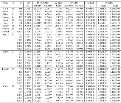
The competing state-of-the-art algorithms that are also applicable to BNs of a moderate size are the Hybrid MCMC method (Eaton and Murphy, 2007) and theK-best algorithm (Tian et al., 2010). The first competing method, the Hybrid MCMC, includes the DP algorithm of Koivisto (2006) (with time complexityO(nk+1C(m)+kn2n)and space complexityO(n2n)) as its first phase and then uses the computed posteriors of all the edges to make the global proposal for its second phase (MCMC phase). When its MCMC phase eventually converges, the Hybrid MCMC will correct the bias coming from the order-prior assumption and provide DAG samples according to the DAG posterior so that the estimator pˆ_⊀(f|D) can be constructed using Eq. (5) for any featuref. The Hybrid MCMC has been empirically shown to converge faster than both the Structure MCMC and the Order MCMC, so that more accurate structure-learning performance can be obtained (Eaton and Murphy, 2007). Note that because the REV-MCMC method (Grzegorczyk and Husmeier, 2008) is shown to be only nearly as efficient as the Order MCMC in the mixing and convergence, the Hybrid MCMC is expected to converge faster than the REV-MCMC method as long asnis moderate so that the Hybrid MCMC is applicable. (But the REV-MCMC method has its own value in learning large BNs since all these methods using some DP technique, including the Hybrid MCMC, theK-best algorithm, and our IW-DDS method, are infeasible for a largenbecause of the space cost.) One limitation of the Hybrid MCMC is that it cannot obtain the interval for p_⊀(f|D) as specified by Theorem 5 (iv). Additionally, the convergence rate of the estimator from the Hybrid MCMC is not theoretically provided by its authors.

The second competing method, the K-best algorithm, applies some DP technique to obtain a collectionG of DAGs with theKbest scores and then uses these DAGs to construct the estimator ˆ

p_⊀(f|D) by Eq. (24) and Eq. (25). One advantage of the K-best algorithm is that its estimator also has the property specified by Theorem 5 (iv) so that it can provide the sound interval for p_⊀(f|D)just as our IW-DDS. However, theK-best algorithm has time complexityO(nk+1C(m)+ T0(K)n2n−1) and space complexity O(Kn2n), where T0(K) is the time spent on the best-first search for K solutions and T0(K) has been shown to be O(KlogK) by Flerova et al. (2012). Thus, the increase inK will dramatically increase the computation cost of theK-best algorithm whennis not small. As a result, to obtain an interval width similar to that from our IW-DDS, much more time and space cost is required for theK-best. In our experiments using an ordinary desktop PC, the computation problem becomes severe for n ≥ 19 becauseK can only take some small values (such as no more than 40) before theK-best algorithm exhausts the memory. Accordingly, ∆obtained from theK-best is usually smaller than that from our IW-DDS (so that the interval from theK-best is usually wider) even ifK is set to reach the memory limit of a computer. (Please refer to Section 4.2 for detailed discussion.)

3.3.1 COMPARISON BETWEENOURBIAS-CORRECTION STRATEGY ANDTHAT OFELLIS AND

WONG(2008)

Our bias-correction strategy used in the IW-DDS solves the computation problem existing in the idea of Ellis and Wong (2008) and ensures the desirable properties of our estimatorpˆ_⊀(f|D)stated in Theorem 5.

Because in the Order MCMC, sampling an order is much more computationally expensive than sampling a DAG given an order, the strategy of Ellis and Wong (2008) emphasizes making the full use of each sampled order≺, that is, keeping drawing DAGs consistent with each sampled≺until the sum of joint probabilities for the unique sampled DAGs,P

proportion (such as95%) ofp(≺, D). Unfortunately, such a strategy has a computational problem when the number of variablesnis not small and the number of data instancesmis small. Because there are a super-exponential number (2Θ(knlog(n))) of DAGs (with the maximum in-degreek) con-sistent with each order (Friedman and Koller, 2003), it is possible that a non-negligible portion of probability massp(≺, D)will be distributed almost uniformly to a majority of these consistent DAGs whenmis small. Consequently,N_G≺, the required number of DAGs sampled per each sam-pled order≺, will be extremely large, leading to large computation cost. For samplingN_G≺DAGs consistent with each sampled order≺, its expected time cost is O(nk+1 +nklog(n)N_G≺) (even if a time-saving strategy as that described in Section 3.2.1 is used) and its memory requirement isO(n2N_G≺). If the memory requirement exceeds the memory of the running computer, the hard disk has to be used to temporarily store the sampled DAGs in some way. (We notice that Ellis and Wong, 2008, limited their experiments to the data sets with at most 14 variables.) If we take the data set “Child” (Tsamardinos et al., 2006) withn = 20andm = 100for example, for an order

≺randomly sampled by our order sampling algorithm, our experiment shows that1×107 DAGs (which contain 932,137 unique DAGs) need to be sampled to let the ratioP

ip(≺, Gi, D)/p(≺, D)

reach94.071%;1.5×107DAGs (which contain 1,204,262 unique DAGs) need to be sampled to let the ratioP

ip(≺, Gi, D)/p(≺, D)reach94.952%. To solve this problem, based on the efficiency

of our order sampling algorithm, our strategy samples only one DAG from each sampled order in the DDS step, so that the large computation cost per each sampled order is avoided for any data set. Meanwhile, unlike the strategy of Ellis and Wong (2008), our strategy does not delete the duplicate order samples. Therefore, if an order≺ gets sampled j (≥ 1)times in the order sampling step, essentiallyjDAGs will be sampled for such a unique order in the DAG sampling step. Thus,j, the number of occurrences, implicitly serves as an importance indicator for≺among the orders.

Furthermore, the strategy of Ellis and Wong (2008) cannot guarantee that the sampled DAGs are independent, even if large computation cost is spent in sampling a huge number of DAGs per each sampled order. This is essentially because multiple DAGs sampled from a fixed order according to the strategy of Ellis and Wong (2008) are not independent. For example, given that a DAGGwith an edgeX →Y gets sampled from an order≺, which implies that nodeXprecedes nodeY in the given order≺, then the conditional probability that any DAGG0 with a reverse edgeY → X gets sampled under the fixed order≺becomes zero, so thatGandG0 are not independent. In general, once the number of sampled orders is fixed, even if the number of sampled DAGs per each sampled order keeps increasing, every DAG that is consistent with none of the sampled orders will still have no chance of getting sampled. In contrast, the sampling strategy in our IW-DDS is able to guarantee the property that all the DAGs sampled from the DDS step are independent, which has been stated in Theorem 3. Such a property is a key to ensuring the good properties of our estimatorpˆ_⊀(f|D) stated in Theorem 5.

4. Experimental Results

We have implemented our algorithms in a C++ language tool called “BNLearner” and run sev-eral experiments to demonstrate its capabilities. (BNLearner is available at http://www.cs.

iastate.edu/˜jtian/Software/BNLearner/BNLearner.htm.) Our tested data sets

syn-thetic data sets: the first one is a synsyn-thetic data set “Syn15” generated from a gold-standard 15-node Bayesian network built by us; the second one is a synthetic data set “Insur19” generated from a 19-node subnetwork of “Insurance” Bayesian network (Binder et al., 1997); the third one is a synthetic data set “Child” from a 20-node “Child” Bayesian network used by Tsamardinos et al. (2006). All the data sets contain only discrete variables (or are discretized) and have no missing values (or have their missing values filled in). For the four data sets (“Syn15,” “Letter,” “Insur19,” and “Child”), because a large number of data instances are available, we also varym(the number of instances) to see the corresponding learning performance. (All the data cases are also included in the tool of BNLearner.) All the experiments in this section were run under Linux on one ordinary desktop PC with a 3.0 GHz Intel Pentium processor and 2.0 GB memory if no extra specification is provided. In addition, the maximum in-degreekwas assumed to be5for all the experiments.

4.1 Experimental Results for the DDS

In this subsection, we compare our DDS algorithm with the Partial Order MCMC method (Niini-maki et al., 2011), the state-of-the-art learning method under the order-modular prior.

The Partial Order MCMC (PO-MCMC) method is implemented in BEANDisco, a C++ lan-guage tool provided by Niinimaki et al. (2011). (BEANDisco is available athttp://www.cs. helsinki.fi/u/tzniinim/BEANDisco/.) The current version of BEANDisco can only estimate the posterior of an edge feature, but as Niinimaki et al. (2011) stated, the PO-MCMC read-ily enables estimating the posterior of any structural feature by further sampling DAGs consistent with an order.

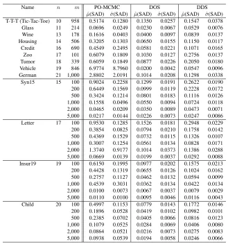
Because n (the number of the variables) in each investigated data case is moderate, we are able to use REBEL, a C++ language implementation of the DP algorithm of Koivisto (2006), to get the exact posterior of every edge under the assumption of the order-modular prior. (REBEL is available athttp://www.cs.helsinki.fi/u/mkhkoivi/REBEL/.) Therefore, we can use the criterion of the sum of the absolute differences (SAD) (Eaton and Murphy, 2007) to measure the feature-learning performance for each data case:

SAD=X

f

|p(f|D)−p(fˆ |D)|,

wherep(f|D)is the exact posterior of the investigated featuref, andp(fˆ |D)is the corresponding estimator. In this subsection, SAD is essentiallyP

ij|p≺(i→ j|D)−p≺(iˆ → j|D)|, because the

investigated feature is the edge featurei → j under the order-modular prior. A smaller SAD will indicate a better performance in structure discovery. Note that the criterion SAD is closely related to another criterion MAD (the mean of the absolute differences), because MAD = SAD/(n(n−1)). Thus, for each data case the conclusion based on the comparison of SAD values is the same as that based on the comparison of MAD values, becausen(n−1)is just a constant for each data case.

For fair comparison, in our algorithms we used the K2 score (Heckerman et al., 1995) and set qi(Ui) = 1andρi(P ai) = 1/ _|n_{P a}−1_i|

for eachi, Ui, andP ai, where|P ai|is the size of the setP ai,

because such a setting is used in both BEANDisco and REBEL.

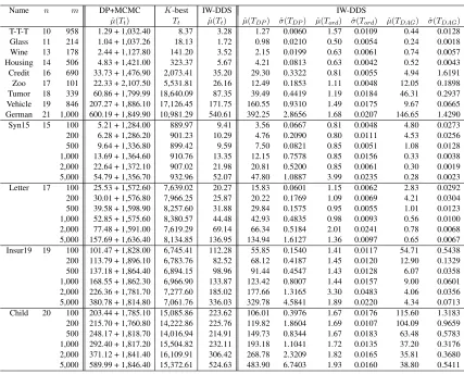
Name n m PO-MCMC DOS DDS

ˆ

µ(SAD) ˆσ(SAD) µˆ(SAD) ˆσ(SAD) µˆ(SAD) ˆσ(SAD) T-T-T (Tic-Tac-Toe) 10 958 0.5174 0.1280 0.1350 0.0257 0.1547 0.0378 Glass 11 214 0.0696 0.0249 0.0230 0.0067 0.0529 0.0076 Wine 13 178 0.1616 0.0403 0.0400 0.0097 0.0839 0.0137 Housing 14 506 0.3205 0.1303 0.0650 0.0155 0.1150 0.0117 Credit 16 690 0.4549 0.2495 0.0581 0.0221 0.1071 0.0165 Zoo 17 101 0.6079 0.1809 0.1030 0.0127 0.2756 0.0137 Tumor 18 339 0.6059 0.1849 0.0877 0.0226 0.2050 0.0180 Vehicle 19 846 6.9774 8.7960 0.0200 0.0042 0.0547 0.0096 German 21 1,000 2.8802 2.0191 0.1014 0.0208 0.1298 0.0338 Syn15 15 100 0.9024 0.2258 0.1299 0.0191 0.2622 0.0190 200 0.6449 0.1569 0.0999 0.0119 0.2228 0.0172 500 0.3424 0.1214 0.0801 0.0183 0.1116 0.0126 1,000 0.1558 0.0496 0.0550 0.0094 0.0724 0.0118 2,000 0.0465 0.0209 0.0350 0.0089 0.0473 0.0071 5,000 0.0217 0.0144 0.0226 0.0073 0.0247 0.0086 Letter 17 100 0.9530 0.1285 0.1526 0.0181 0.2948 0.0229 200 0.3854 0.0825 0.0794 0.0210 0.1758 0.0142 500 0.4369 0.1529 0.0732 0.0115 0.1326 0.0107 1,000 0.3007 0.1254 0.0561 0.0134 0.0828 0.0171 2,000 1.3740 0.9177 0.1014 0.0373 0.1386 0.0288 5,000 0.0669 0.0139 0.0199 0.0037 0.0292 0.0088 Insur19 19 100 0.6150 0.1995 0.0977 0.0202 0.1575 0.0213 200 0.4428 0.1319 0.0655 0.0126 0.1024 0.0162 500 0.2757 0.1127 0.0462 0.0132 0.0594 0.0099 1,000 0.4539 0.3031 0.0362 0.0134 0.0422 0.0134 2,000 0.0100 0.0073 0.0067 0.0037 0.0079 0.0029 5,000 0.0110 0.0100 0.0095 0.0046 0.0116 0.0043 Child 20 100 0.4997 0.1153 0.0779 0.0143 0.1772 0.0146 200 0.1896 0.0528 0.0419 0.0102 0.0982 0.0101 500 0.2385 0.0702 0.0405 0.0066 0.0816 0.0123 1,000 0.1079 0.0525 0.0284 0.0069 0.0406 0.0080 2,000 0.0864 0.0521 0.0216 0.0073 0.0275 0.0083 5,000 0.0938 0.0539 0.0194 0.0058 0.0246 0.0066

Table 1: Comparison of the PO-MCMC, the DOS, and the DDS in Terms of SAD

ran the first 10,000 iterations for “burn-in,” and then took 200 partial-order samples at intervals of50 iterations. Thus, there were 20,000 iterations in total. (The time cost of each iteration in the PO-MCMC is O(nk+1 +n22bn/b).) In the PO-MCMC, for each sampled partial order Pi,

p(f|D, Pi)is obtained byp(D, f, Pi)/p(D, Pi) =p(D, f, Pi)/p(D, f ≡1, Pi), wherep(D, f, Pi)

=P

≺⊇Pi

P

G⊆≺f(G)p(≺, G)p(D|G). The notation

P

≺⊇Pimeans that all the total orders (≺’s) that are linear extensions of the sampled partial orderPiwill be included to obtainp(D, f, Pi). For

example, for a data set withn = 20, because our bucket sizeb = 10, there are 20!/(10!10!) = 184,756 total orders that will be included for each sampled partial orderPi. The inclusion of the

information of a large number of total orders consistent with each sampled partial order gives great learning power to the PO-MCMC method; such an inclusion can be efficiently computed by the algorithm of Parviainen and Koivisto (2010) with the assumptions of the order-modular prior and the maximum in-degree k. Finally, for the PO-MCMC, the estimated posterior of each edge is computed usingp≺(fˆ |D) = (1/T)PT

i=1p(f|D, Pi).

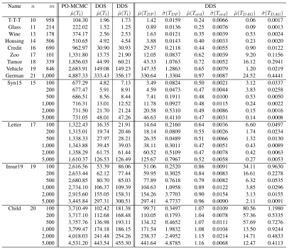
Name n m PO-MCMC DOS DDS DDS

ˆ

µ(Tt) µˆ(Tt) µˆ(Tt) µˆ(TDP) σˆ(TDP) µˆ(Tord) ˆσ(Tord) µˆ(TDAG) σˆ(TDAG)

T-T-T 10 958 104.30 1.96 1.73 1.42 0.0159 0.24 0.0066 0.06 0.0017 Glass 11 214 222.02 1.52 1.25 0.89 0.0136 0.25 0.0076 0.09 0.0013 Wine 13 178 374.17 2.56 2.53 1.63 0.0121 0.35 0.0039 0.53 0.0024 Housing 14 506 510.65 4.92 4.54 3.88 0.0143 0.40 0.0033 0.23 0.0020 Credit 16 690 962.97 30.90 30.93 29.57 0.2118 0.44 0.0055 0.90 0.0122 Zoo 17 101 1,331.80 13.75 21.90 12.05 0.0837 0.62 0.0039 9.20 0.1156 Tumor 18 339 1,856.03 44.99 60.21 43.33 1.0763 0.72 0.0052 16.12 0.2941 Vehicle 19 846 2,683.91 149.08 149.23 147.35 1.2863 0.65 0.0079 1.20 0.0219 German 21 1,000 4,887.33 333.43 356.17 330.64 1.3304 0.97 0.0087 24.52 0.4441 Syn15 15 100 677.29 4.82 7.13 3.49 0.0824 0.50 0.0021 3.12 0.0337 200 677.47 5.91 8.91 4.59 0.0473 0.47 0.0044 3.83 0.0258 500 686.51 8.56 8.44 7.41 0.1911 0.48 0.0100 0.53 0.0050 1,000 716.31 13.01 12.52 11.78 0.0927 0.48 0.0115 0.24 0.0022 2,000 731.50 21.70 21.24 20.58 0.5310 0.49 0.0086 0.15 0.0016 5,000 731.05 48.01 47.26 46.63 0.4110 0.47 0.0031 0.14 0.0008 Letter 17 100 1,322.43 16.35 21.91 14.64 0.2160 0.64 0.0036 6.60 0.0497 200 1,315.01 19.74 20.46 18.14 0.0809 0.55 0.0026 1.74 0.0234 500 1,338.33 27.97 28.21 26.35 0.0489 0.51 0.0066 1.32 0.0130 1,000 1,343.88 39.45 39.03 38.11 0.3011 0.47 0.0051 0.43 0.0089 2,000 1,358.29 61.75 61.44 60.52 0.5109 0.47 0.0078 0.42 0.0063 5,000 1,610.37 126.53 126.49 125.67 0.7967 0.52 0.0058 0.27 0.0053 Insur19 19 100 2,616.56 53.39 86.06 51.06 0.2520 0.86 0.0091 34.11 0.9630 200 2,633.44 62.12 77.44 59.95 0.3025 0.84 0.0083 16.61 0.2278 500 2,680.85 80.70 85.03 77.89 0.7618 0.79 0.0082 6.32 0.0535 1,000 2,734.10 106.37 109.39 104.63 1.0958 0.89 0.0122 3.85 0.0296 2,000 2,915.60 155.05 158.31 154.26 3.7703 0.90 0.0154 3.13 0.0155 5,000 3,445.84 297.31 300.51 297.41 4.7737 0.96 0.0090 2.11 0.0091 Child 20 100 3,710.49 102.42 181.38 99.71 0.3497 1.07 0.0109 80.56 1.1980 200 3,717.10 112.68 168.48 110.05 0.1793 1.04 0.0078 57.36 0.5335 500 3,757.76 136.98 193.11 134.32 0.4652 1.07 0.0111 57.69 0.7276 1,000 3,799.47 174.18 186.15 171.54 1.9832 1.08 0.0104 13.50 0.9244 2,000 4,018.03 241.48 254.26 238.37 2.4952 1.15 0.0214 14.71 0.4833 5,000 4,531.20 443.54 455.30 441.64 4.8785 1.16 0.0068 12.47 0.4113

Table 2: Comparison of the PO-MCMC, the DOS, and the DDS in Terms of Time (in Seconds)

is, 20,000 (total) orders were sampled. Theoretically, we expect that the learning performance of the DOS should be better than that of the DDS because the additional approximation coming from the DAG sampling step is avoided by the DOS. By listing the performance of the DOS, we mainly intend to examine how much the performance of the DDS decreases because of the additional approximation from sampling one DAG per order. Nevertheless, because the DDS but not the DOS is capable of learning non-modular features, the comparison between the PO-MCMC method and the DDS method is our main task.

Table 1 shows the experimental results in terms of SAD for each data case withnvariables and minstances, and Table 2 lists the running-time cost corresponding to Table 1. For each of the three methods, we performed 15 independent runs for each data case. The sample mean and the sample standard deviation of the 15 SAD values of each method, denoted by µ(SAD) andˆ ˆσ(SAD), are listed in Table 1. Correspondingly, the sample mean of the total running timeTtof each method,

denoted byµ(Tˆ t), is shown in Table 2. (Precisely speaking, the reported total running timeTtof

the reported total running timeTtof the DOS method also includes the relatively tinyO(No)time

cost of computingp≺(fˆ |D)for each edgef using Eq. 17 and Eq. 15 at the end.) In addition, the sample mean and the sample standard deviation of the running time of the three steps of the DDS (including the DP step, the order sampling step, and the DAG sampling step), denoted byµ(Tˆ DP),

ˆ

σ(TDP),µ(Tˆ ord),σ(Tˆ ord),µ(Tˆ DAG), andσ(Tˆ DAG)respectively, are listed in the last six columns

of Table 2. Note that we still showµ(Tˆ DP), the mean running time of the DP step of the DDS in the

15 independent runs, though the DP step is not a random algorithm at all. The running time of the DP step is not exactly the same in each run because of the randomness from uncontrolled factors such as the internal status of the computer. By showingµ(Tˆ DP), we can clearly see the percentage

of the total running time that the DP step typically takes by comparingµ(Tˆ DP)andµ(Tˆ t).

Tables 1 and 2 clearly illustrate the performance advantage of our DDS method over the PO-MCMC method. The overall time cost of our DDS based on 20,000 DAG samples is much smaller than the corresponding cost of the PO-MCMC method based on 20,000 MCMC iterations in the partial-order space. Using much shorter time, our DDS method has itsµ(SAD) much smaller thanˆ ˆ

µ(SAD) from the PO-MCMC method for 28 out of all the 33 data cases. The five exceptional cases are Glass, Syn15 withm =2,000, Syn15 withm =5,000, Insur19 withm =2,000, and Insur19 with m = 5,000. (In both Glass and Insur19 withm =2,000, µ(SAD) using our DDS methodˆ is still smaller than that using the PO-MCMC method, but their difference is not large compared withσ(SAD) from the PO-MCMC method.) Furthermore, because bothˆ µ(SAD) andˆ σ(SAD) areˆ given in Table 1, by the two-samplettest with unequal variances (Casella and Berger, 2002), we can conclude with strong evidence (at the significance level5×10−3) that the real mean of SAD using our DDS method is smaller than the real mean of SAD using the PO-MCMC method for each of the 28 data cases. For the exceptional data case Glass, the p-value of thettest is0.012, so that we can conclude at the significance level0.05that the real mean of SAD using our DDS method is smaller than that using the PO-MCMC method. For each of the other four exceptions, by the same ttest we cannot reject (with the p-value> 0.2) the null hypothesis that there is no difference in the real means of SAD from the two methods. (Corresponding to Table 1, the comparison is also re-demonstrated using boxplots in the supplementary material for all the 33 data cases.) Thus, the advantage of our DDS algorithm over the PO-MCMC method in learning Bayesian networks of a moderatencan be clearly seen, though the value of the PO-MCMC method still remains for larger nfor which our DDS algorithm is infeasible.

In terms of the total running time of the DDS algorithm, Table 2 shows that the running time of the DP step always accounts for the largest portion. The running time of the DAG sampling step is less than 81 seconds to get 20,000 DAG samples for all the 33 cases. Though both the order sampling step and the DAG sampling step involve randomness, the variability of their running time is actually small. This can be seen from the ratio ofσ(Tˆ ord)toµ(Tˆ ord)(which is always less

than3.04%for all the 33 cases) and the ratio ofσ(Tˆ DAG)toµ(Tˆ DAG)(which is always less than

6.85%for all the 33 cases). The ratio of µ(Tˆ DAG) to µ(Tˆ ord) ranges from0.25 to75.29 across

the 33 cases, which is much smaller than the upper bound of the ratio ofO(nk+1No)toO(n2No).

second, a93.48%of decrease. In summary, the effectiveness of our time-saving strategy introduced in Section 3.2.1 has been clearly shown in Table 2.

In addition, Table 1 clearly shows that the learning performance of the DOS is better than that of the DDS, as expected theoretically. Note thatµ(SAD) from the DOS is significantly smaller thanˆ ˆ

µ(SAD) from the DDS for 28 out of the 33 data cases. The five other cases are Tic-Tac-Toe, Syn15 withm =5,000, and Insur19 withm =1,000, 2,000, and 5,000. For each of these 28 data cases, by the two-samplettest with unequal variances (Casella and Berger, 2002), we can conclude (at the significance level0.05) that the real mean of SAD using the DOS is smaller than that using the DDS. This shows that the additional approximation from the DAG sampling step will usually make the DDS perform worse than the DOS in learning modular features. Nevertheless, the DDS but not the DOS has the ability of learning arbitrary non-modular features, which is the main goal of this paper.

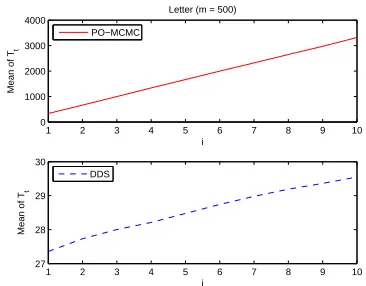
Finally, we present the experimental results for the DDS by varying the sample size. We first choose the data case Letter withm = 500as an example. For the DDS, we tried the sample size No =5,000·i, where i ∈ {1,2, . . . ,10}. For eachi, we independently ran the DDS15 times to

get the sample mean and the sample standard deviation of SAD for the (directed) edge features. For the PO-MCMC, with the bucket sizeb = 10, we ran totally 5,000·iMCMC iterations in the partial-order space, wherei ∈ {1,2, . . . ,10}. For eachi, we discarded the first 2,500·iMCMC iterations for “burn-in” and set the thinning parameter to be50, so that50·ipartial orders finally got sampled. Again, for eachi, we independently ran the PO-MCMC15times to get the sample mean and the sample standard deviation of SAD for the edge features.

Figure 1 shows the SAD performance of the two methods with each i in terms of the edge features, where an error bar represents one sample standard deviationσ(SAD) acrossˆ 15runs from a method (the PO-MCMC or the DDS) at eachi. For example, Figure 1 shows that wheni = 4, ˆ

µ(SAD)= 0.1326andσ(SAD)ˆ = 0.0107from our DDS algorithm;µ(SAD)ˆ = 0.4369andσ(SAD)ˆ = 0.1529from the PO-MCMC method. This exactly matches the results previously shown in Table 1. Correspondingly, Figure 2 showsµ(Tˆ t)(the sample mean of the total running time) of the

PO-MCMC and the DDS with eachi, where the running time is in seconds. The advantage of our DDS can be clearly seen from Figures 1 and 2. For eachi∈ {1,2, . . . ,10}, the real mean of SAD from the DDS is significantly smaller than that from the PO-MCMC with the p-value<5×10−3returned by the two-samplettest (with unequal variances). Meanwhile, the total running time of the DDS is much shorter than that of the PO-MCMC. For example,µ(Tˆ t)of the DDS increases with respect to

iand reaches only29.55seconds ati= 10. This is shorter than9%ofµ(Tˆ t)of the PO-MCMC at

i= 1, which is336.09seconds. Therefore, the learning performance of the DDS with each sample size is significantly better than that of the PO-MCMC for the data case Letter withm= 500.

We also performed the experiment with the same experimental settings for the data cases Tic-Tac-Toe, Wine, Child withm= 500, and German. Please refer to the supplementary material for the experimental results. (The supplementary material is available athttp://www.cs.iastate.

edu/˜jtian/Software/BNLearner/BN_Learning_Sampling_Supplement.pdf. )