Efficient Feature Selection via Analysis of
Relevance and Redundancy
Lei Yu [email protected]
Huan Liu [email protected]
Department of Computer Science & Engineering Arizona State University
Tempe, AZ 85287-8809, USA
Editor: Isabelle Guyon
Abstract
Feature selection is applied to reduce the number of features in many applications where data has hundreds or thousands of features. Existing feature selection methods mainly focus on finding rele-vant features. In this paper, we show that feature relevance alone is insufficient for efficient feature selection of high-dimensional data. We define feature redundancy and propose to perform explicit redundancy analysis in feature selection. A new framework is introduced that decouples relevance analysis and redundancy analysis. We develop a correlation-based method for relevance and redun-dancy analysis, and conduct an empirical study of its efficiency and effectiveness comparing with representative methods.
Keywords: supervised learning, feature selection, relevance, redundancy, high dimensionality
1. Introduction
In classic supervised learning, one is given a training set of labeled fixed-length feature vectors (instances). An instance is typically described as an assignment of values f = (f1, ...,fN)to a set
of features F= (F1, ...,FN)and one of l possible classes c1, ...,cl to the class label C. The task is to
induce a hypothesis (classifier) that accurately predicts the labels of novel instances. The learning of the classifier is inherently determined by the feature-values. In theory, more features should provide more discriminating power, but in practice, with a limited amount of training data, excessive features will not only significantly slow down the learning process, but also cause the classifier to over-fit the training data as irrelevant or redundant features may confuse the learning algorithm.
Feature selection has been an active and fruitful field of research and development for decades in statistical pattern recognition (Mitra et al., 2002), machine learning (Liu et al., 2002b; Robnik-Sikonja and Kononenko, 2003), data mining (Kim et al., 2000; Dash et al., 2002) and statistics (Hastie et al., 2001; Miller, 2002). It has proven in both theory and practice effective in enhancing learning efficiency, increasing predictive accuracy, and reducing complexity of learned results (Almuallim and Dietterich, 1994; Koller and Sahami, 1996; Blum and Langley, 1997). Let G be some subset of
F and fGbe the value vector of G. In general, the goal of feature selection can be formalized as
se-lecting a minimum subset G such that P(C|G=fG)is equal or as close as possible to P(C|F= f),
Example 1 (Optimal subset) Let features F1, ...,F5be Boolean. The target concept is C=g(F1,F2)
where g is a Boolean function. With F2=F3 and F4=F5, there are only eight possible instances.
In order to determine the target concept, F1 is indispensable; one of F2 and F3 can be disposed of
(note that C can also be determined by g(F1, F3)), but we must have one of them; both F4and F5
can be discarded. Either{F1,F2}or{F1,F3}is an optimal subset. The goal of feature selection is
to find either of them.
In the presence of hundreds or thousands of features, researchers notice (Yang and Pederson, 1997; Xing et al., 2001) that it is common that a large number of features are not informative because they are either irrelevant or redundant with respect to the class concept. In other words, learning can be achieved more efficiently and effectively with just relevant and non-redundant features. However, the number of possible feature subsets grows exponentially with the increase of dimensionality. Finding an optimal subset is usually intractable (Kohavi and John, 1997) and many problems related to feature selection have been shown to be NP-hard (Blum and Rivest, 1992).
Researchers have studied various aspects of feature selection. One of the key aspects is to measure the goodness of a feature subset in determining an optimal one (Liu and Motoda, 1998). Different feature selection methods can be broadly categorized into the wrapper model (Kohavi and John, 1997; Kim et al., 2000) and the filter model (Liu and Setiono, 1996; Liu et al., 2002b; Hall, 2000; Yu and Liu, 2003). The wrapper model uses the predictive accuracy of a predetermined learning algorithm to determine the goodness of the selected subsets. These methods are compu-tationally expensive for data with a large number of features (Kohavi and John, 1997). The filter model separates feature selection from classifier learning and selects feature subsets that are inde-pendent of any learning algorithm. It relies on various measures of the general characteristics of the training data such as distance, information, dependency, and consistency (Liu and Motoda, 1998).
Search is another key problem in feature selection. To balance the tradeoff of result optimality and
computational efficiency, different search strategies such as complete, heuristic, and random search have been studied to generate candidate feature subsets for evaluation (Blum and Langley, 1997; Dash and Liu, 2003). According to the availability of class labels, there are feature selection meth-ods for supervised learning (Dash and Liu, 1997; Yu and Liu, 2003) as well as for unsupervised
learning (Kim et al., 2000; Dash et al., 2002). Feature selection has found success in many
applica-tions like text categorization (Yang and Pederson, 1997; Forman, 2003), image retrieval (Swets and Weng, 1995; Dy et al., 2003), genomic microarray analysis (Xing et al., 2001; Yu and Liu, 2004), customer relationship management (Ng and Liu, 2000), and intrusion detection (Lee et al., 2000).
irrelevant features as well as redundant ones. However, among existing heuristic search strategies for subset evaluation, even greedy sequential search which reduces the search space from O(2N)to
O(N2)can become very inefficient for high-dimensional data. The limitations of existing research clearly suggest that we should pursue a different framework of feature selection that allows efficient analysis of both feature relevance and redundancy for high-dimensional data.
The remainder of this paper is organized as follows. In Section 2, we review notions of feature relevance, identify the need for redundancy analysis, and provide a formal definition of feature redundancy. In Section 3, we analyze in detail the limitations of current approaches and propose a new framework of efficient feature selection. In Section 4, we describe correlation measures, and present a correlation-based method for efficient relevance and redundancy analysis under the new framework. Section 5 contains an empirical study of our method in terms of efficiency and effectiveness comparing with representative methods. Section 6 concludes this work and points out some future directions.
2. Feature Relevance and Feature Redundancy
Traditionally, feature selection research has focused on searching for relevant features. Although some recent work has pointed out the existence and effect of feature redundancy (Koller and Sa-hami, 1996; Kohavi and John, 1997; Hall, 2000), there is little work on explicit treatment of feature redundancy. In the following, we first present a classic notion of feature relevance and illustrate why it alone cannot handle feature redundancy, and then provide our formal definition of feature redundancy which paves the way for efficient elimination of redundant features.
2.1 Feature Relevance
Based on a review of previous definitions of feature relevance, John, Kohavi, and Pfleger classified features into three disjoint categories, namely, strongly relevant, weakly relevant, and irrelevant features (John et al., 1994). Let F be a full set of features, Fi a feature, and Si=F− {Fi}. These
categories of relevance can be formalized as follows.
Definition 1 (Strong relevance) A feature Fiis strongly relevant iff
P(C|Fi, Si)6=P(C|Si).
Definition 2 (Weak relevance) A feature Fi is weakly relevant iff
P(C|Fi, Si) =P(C|Si), and
∃S0i⊂Si, such that P(C|Fi, S0i)6=P(C|S0i).
Corollary 1 (Irrelevance) A feature Fiis irrelevant iff
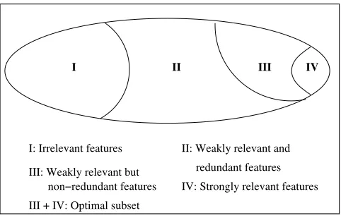
Strong relevance of a feature indicates that the feature is always necessary for an optimal subset; it cannot be removed without affecting the original conditional class distribution. Weak relevance suggests that the feature is not always necessary but may become necessary for an optimal subset at certain conditions. Irrelevance (following Definitions 1 and 2) indicates that the feature is not necessary at all. According to these definitions, it is clear that in previous Example 1, feature F1is strongly relevant, F2, F3weakly relevant, and F4, F5irrelevant. An optimal subset should include all strongly relevant features, none of irrelevant features, and a subset of weakly relevant features. However, it is not given in the definitions which of weakly relevant features should be selected and which of them removed. Therefore, it is necessary to define feature redundancy among relevant features.
2.2 Defining Feature Redundancy
Notions of feature redundancy are normally in terms of feature correlation. It is widely accepted that two features are redundant to each other if their values are completely correlated (for example, features F2and F3 in Example 1). In reality, it may not be so straightforward to determine feature redundancy when a feature is correlated (perhaps partially) with a set of features. We now formally define feature redundancy in order to devise an approach to explicitly identify and eliminate redun-dant features. Before we proceed, we first introduce the definition of a feature’s Markov blanket given by Koller and Sahami (1996).
Definition 3 (Markov blanket) Given a feature Fi, let Mi⊂F(Fi∈/Mi), Miis said to be a Markov blanket for Fiiff
P(F−Mi− {Fi},C|Fi,Mi) =P(F−Mi− {Fi},C|Mi).
The Markov blanket condition requires that Mi subsume not only the information that Fi has
about C, but also about all of the other features. It is pointed out in Koller and Sahami (1996) that an optimal subset can be obtained by a backward elimination procedure, known as Markov blanket
filtering: let G be the current set of features (G=F in the beginning), at any phase, if there exists
a Markov blanket for Fiwithin the current G, Fi is removed from G. It is proved that this process
guarantees a feature removed in an earlier phase will still find a Markov blanket in any later phase, that is, removing a feature in a later phase will not render the previously removed features necessary to be included in the optimal subset. According to previous definitions of feature relevance, we can also prove that strongly relevant features cannot find any Markov blanket. Since irrelevant features should be removed anyway, we exclude them from our definition of redundant features.
Definition 4 (Redundant feature) Let G be the current set of features, a feature is redundant and hence should be removed from G iff it is weakly relevant and has a Markov blanket Miwithin G .
III IV
I: Irrelevant features
IV: Strongly relevant features II: Weakly relevant and
III + IV: Optimal subset
redundant features non−redundant features
III: Weakly relevant but
I II
Figure 1: A view of feature relevance and redundancy.
3. Efficient Feature Selection via Relevance and Redundancy Analysis
We now review two major approaches in dealing with feature relevance and redundancy, analyze their limitations for high-dimensional data, and then propose a new framework of efficient feature selection based on relevance and redundancy analysis.
3.1 Existing Approaches in Dealing with Relevance and Redundancy
As mentioned earlier, there exist two major approaches in feature selection: individual evaluation and subset evaluation. Individual evaluation, also known as feature weighting/ranking (Blum and Langley, 1997; Guyon and Elisseeff, 2003), assesses individual features and assigns them weights according to their degrees of relevance. A subset of features is often selected from the top of a ranking list, which approximates the set of relevant features (II, III, and IV in Figure 1). With its linear time complexity in terms of dimensionality N, this approach is efficient for high-dimensional data. However, it is incapable of removing redundant features because redundant features likely have similar rankings. As long as features are deemed relevant to the class, they will all be selected even though many of them are highly correlated to each other. For high-dimensional data which may contain a large number of redundant features, this approach may produce results far from optimal.
sub-sets required in the subset generation step. Although there exist various heuristic search strategies such as greedy sequential search, best-first search, and genetic algorithm (Liu and Motoda, 1998), most of them still incur time complexity O(N2), which prevents them from scaling well to data sets containing tens of thousands of features.
Subset Generation
Subset Evaluation
Stopping Criterion Original
Set
Current Best Subset Candidate
Subset
Selected Subset Yes No
Figure 2: A traditional framework of feature selection.
3.2 A New Framework of Efficient Feature Selection
From previous discussions, it is clear that in order to eliminate redundant features, the state-of-the-art feature selection methods have to rely on the approach of subset evaluation which implicitly handles feature redundancy with feature relevance. These methods can produce better results than methods without handling feature redundancy, but the high computational cost of the subset search makes them inefficient for high-dimensional data. Therefore, in our solution, we propose a new framework of feature selection which avoids implicitly handling feature redundancy and turns to efficient elimination of redundant features via explicitly handling feature redundancy.
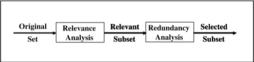
Relevance definitions divide features into strongly relevant, weakly relevant, and irrelevant ones; redundancy definition further divides weakly relevant features into redundant and non-redundant ones. Our goal is to efficiently find the optimal subset (parts III and IV in Figure 1). We can achieve this goal through a new framework of feature selection (shown in Figure 3) composed of two steps: first, relevance analysis determines the subset of relevant features by removing irrelevant ones, and second, redundancy analysis determines and eliminates redundant features from relevant ones and thus produces the final subset. Its advantage over the traditional framework of subset evaluation lies in that by decoupling relevance and redundancy analysis, it circumvents subset search and allows a both efficient and effective way in finding a subset that approximates an optimal subset.
Relevance Analysis
Redundancy Analysis Original
Set
Relevant Subset Relevant
Subset
Selected Subset Selected
Subset
It is sensible to use efficient heuristic methods to approximate the computation of relevant fea-tures and redundant feafea-tures under our new framework for two reasons. On one hand, searching for an optimal subset based on the definitions of feature relevance and redundancy is combinatorial in nature. It is obvious that exhaustive or complete search is prohibitive with a large number of features. On the other hand, an optimal subset is defined based on the full population where the true data distribution is known. It is generally assumed (Mitchell, 1997; Miller, 2002) that a training data set is only a small portion of the full population, especially in a high-dimensional space. Therefore, it is not proper to search for an optimal subset from the training data as over-searching the training data can cause over-fitting (Jensen and Cohen, 2000). We next present our approximation method.
4. A Correlation Based Method
Correlation is widely used in machine learning and statistics for relevance analysis. In this section, we first introduce our choice of correlation measure in Section 4.1, then describe our correlation-based method for both relevance and redundancy analysis in Section 4.2, and present and analyze the algorithm in Section 4.3.
4.1 Correlation Measures
There exist broadly two types of measures for the correlation between two random variables: linear and non-linear. Of linear correlation, the most well known measure is linear correlation coefficient. For a pair of variables(X,Y), the linear correlation coefficientρis given by
ρ=
∑
i
(xi−xi)(yi−yi)
q ∑
i
(xi−xi)2
q ∑
i
(yi−yi)2 ,
where xi is the mean of X , and yiis the mean of Y . The value ofρlies between -1 and 1, inclusive.
If X and Y are completely correlated,ρtakes the value of 1 or -1; if X and Y are independent,ρis zero. It is a symmetrical measure for two variables. Other measures in this category are basically variations of the above formula, such as least square regression error and maximal information
compression index (Mitra et al., 2002). However, it is not safe to always assume linear correlation
between features in the real world. Linear correlation measures may not be able to capture corre-lations that are not linear in nature. It can also be observed that linear correlation coefficient is not suitable for nominal data.
Among non-linear correlation measures, many measures are based on the information-theoretical concept of entropy, a measure of the uncertainty of a random variable. The entropy of a variable X is defined as
H(X) =−
∑
iP(xi)log2(P(xi)),
and the entropy of X after observing values of another variable Y is defined as
H(X|Y) =−
∑
jP(yj)
∑
iP(xi|yj)log2(P(xi|yj)),
where P(xi)is the prior probabilities for all values of X , and P(xi|yi)is the posterior probabilities
information about X provided by Y and is called information gain (Quinlan, 1993), given by
IG(X |Y) =H(X)−H(X|Y).
According to this measure, feature Y is regarded more correlated to feature X than to feature Z, if IG(X |Y)>IG(Z |Y). It is easy to prove that information gain is a symmetrical measure. Symmetry is a desired property for a measure of correlations between features. It ensures that the order of two features ((X,Y ) or (Y,X )) will not affect the value of the measure. Since information
gain tends to favor features with more values, it should be normalized with their corresponding entropy. Therefore, we choose symmetrical uncertainty (Press et al., 1988), defined as
SU(X,Y) =2
IG(X |Y)
H(X) +H(Y)
.
It compensates for information gain’s bias toward features with more values and restricts its values to the range [0,1]. A value of 1 indicates that knowing the values of either feature completely predicts the values of the other; a value of 0 indicates that X and Y are independent. In addition, it still treats a pair of features symmetrically. Entropy-based measures handle nominal or discrete features, and therefore continuous features need to be properly discretized (Liu et al., 2002a) in order to use entropy-based measures.
4.2 Efficient Relevance and Redundancy Analysis
Using symmetrical uncertainty (SU ) as the correlation measure, we are ready to develop an approx-imation method for both relevance and redundancy analysis under our new framework introduced in Section 3.2. We first differentiate two types of correlation between features (including the class).
Definition 5 (C-correlation) The correlation between any feature Fi and the class C is called C-correlation, denoted by SUi,c.
Definition 6 (F-correlation) The correlation between any pair of features Fiand Fj(i6=j)is called F-correlation, denoted by SUi,j.
Aiming to achieve high efficiency, we calculate C-correlation for each feature, and heuristically decide a feature Fi to be relevant if it is highly correlated with the class C, i.e., if SUi,c>γ, where
γ is a relevance threshold which can be determined by users. The selected relevant features are then subject to redundancy analysis. Similarly, we can evaluate the correlation between individ-ual features for redundancy analysis without considering the correlation between various feature subsets. However, there are two difficulties in determining feature redundancy via pair-wise F-correlation calculation: (1) when two features are not completely correlated with each other, it may be hard to determine feature redundancy and which one to be removed; and (2) it may still require
F-correlation calculation for a total of N(N2−1)pairs, which is inefficient for high-dimensional data. Below, we try to efficiently determine feature redundancy by substantially reducing the number of feature pairs evaluated for F-correlation.
by itself more information about the class than a feature with a smaller C-correlation value. We determine the existence of an approximate Markov blanket between a pair of correlated features
Fi and Fj based on their F-correlation level SUi,j as follows. When SUj,c≥SUi,c, we choose to
evaluate whether feature Fj can form an approximate Markov blanket for feature Fi (instead of Fi
for Fj) in order to maintain more information about the class. In addition, we heuristically use SUi,c
as a threshold to determine whether the F-correlation SUi,jis strong or not. An approximate Markov
blanket can be defined as follows.
Definition 7 (Approximate Markov blanket) For two relevant features Fiand Fj(i6=j), Fjforms an approximate Markov blanket for Fiiff SUj,c≥SUi,cand SUi,j≥SUi,c.
Recall that Markov blanket filtering, a backward elimination procedure based on a feature’s Markov blanket in the current set, guarantees that a redundant feature removed in an earlier phase will still find a Markov blanket in any later phase when another redundant feature is removed. It is easy to verify that this is not the case for backward elimination based on a feature’s approximate Markov blanket in the current set. For instance, if Fj is the only feature that forms an approximate
Markov blanket for Fi, and Fkforms an approximate Markov blanket for Fj, after removing Fibased
on Fj, further removing Fj based on Fk will result in no approximate Markov blanket for Fiin the
current set. However, we can avoid this situation by removing a feature only when it can find an approximate Markov blanket formed by a predominant feature, defined as follows.
Definition 8 (Predominant feature) A relevant feature is predominant iff it does not have any approximate Markov blanket in the current set.
Predominant features will not be removed at any stage. If a feature Fi is removed based on
a predominant feature Fj in an earlier phase, it is guaranteed that it will still find an approximate
Markov blanket (the same Fj) in any later phase when another feature is removed. To summarize,
our method for redundancy analysis consists of (1) selecting a predominant feature, (2) removing all features for which it forms an approximate Markov blanket, and (3) iterating steps (1) and (2) until no more predominate features can be selected. An optimal subset can therefore be approximated by a set of predominant features.
4.3 Algorithm and Analysis
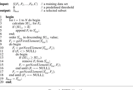
The approximation method for relevance and redundancy analysis presented before can be realized by an algorithm, named FCBF (Fast Correlation-Based Filter). It involves two connected steps: (1) selecting a subset of relevant features, and (2) selecting predominant features from relevant ones. As shown in Figure 4, for a data set S with N features and class C, the algorithm finds a set of predominant features Sbest. In the first step (lines 2-7), it calculates the SU value for each
feature, selects relevant features into S0list based on a predefined thresholdδ, and orders them in a descending order according to their SU values. In the second step (lines 8-18), it further processes the ordered list Slist0 to select predominant features. A feature Fj that has already been determined
to be a predominant feature can always be used to filter out other features for which Fj forms an
input: S(F1,F2, ...,FN,C) // a training data set
δ // a predefined threshold
output: Sbest // a selected subset
1 begin
2 for i=1 to N do begin 3 calculate SUi,cfor Fi;
4 if(SUi,c>δ)
5 append Fito S0list;
6 end;
7 order Slist0 in descending SUi,cvalue;
8 Fj=getFirstElement(S0list);
9 do begin
10 Fi=getNextElement(S0list,Fj);
11 if (Fi<>NULL)
12 do begin
13 if (SUi,j≥SUi,c)
14 remove Fifrom S0list;
15 Fi=getNextElement(S0list,Fi);
16 end until (Fi==NULL);
17 Fj=getNextElement(S0list,Fj);
18 end until (Fj==NULL);
19 Sbest=S0list;
20 end;
Figure 4: FCBF Algorithm.
for Fi(line 13), Fi will be removed from S0list. After one round of filtering features based on Fj, the
algorithm will take the remaining feature right next to Fjas the new reference (line 17) to repeat the
filtering process. The algorithm stops until no more predominant features can be selected. Figure 5 illustrates how predominant features are selected with the rest features removed as redundant ones. In Figure 5, six features are selected as relevant ones and ranked according to their C-correlation values, with F1 being the most relevant one. In the first round, F1 is selected as a predominant feature, and F2 and F4 are removed based on F1. In the second round, F3 is selected, and F6 is removed based on F3. In the last round, F5is selected.
F
1
F
2F
3F
4F
5F
6F
1
F
2F
3F
4F
5F
F
66Figure 5: Selection of predominant features
determine predominant features from relevant ones (assuming all features are selected as relevant ones), it has a best-case complexity O(N)when only one feature is selected and all of the rest of the features are removed, and a worse-case complexity O(N2)when all features are selected. These time complexity results are comparable to subset evaluation based on greedy sequential search in which features are, one at a time, added to the current subset (i.e., sequential forward selection) or removed from the current subset (i.e., sequential backward elimination). However, in general cases when k (1<k<N)features are selected, the number of evaluations performed by FCBF will typically be much less (and certainly never more) than the number of evaluations performed by greedy sequential search because features removed in each round are not considered in the next round and FCBF typically removes a large number of features (instead of only one by greedy sequential search) in each round. This makes FCBF substantially faster than algorithms of subset evaluation based on greedy sequential search, as will be demonstrated by the running time comparisons reported in Section 5. The more features removed in an earlier round, the faster FCBF is. Moreover, selecting a subset of relevant features in the first step can further improves its efficiency.
In summary, our method approximates relevance and redundancy analysis by selecting all pre-dominant features and removing the rest features. It uses both C- and F-correlations to determine feature redundancy and combines sequential forward selection with elimination so that it not only circumvents full pair-wise F-correlation analysis but also achieves higher efficiency than pure se-quential forward selection or backward elimination. However, our method is suboptimal due to the way C- and F-correlations are used for relevance and redundancy analysis and the approximates that it uses. It is fairly straightforward to improve the optimality of the results by considering differ-ent combinations of features in evaluating feature relevance and redundancy, which in turn increases time complexity. Another way to improve result optimality is to find better heuristics in determining a feature’s approximate Markov blanket.
5. Empirical Study
In this section, we empirically evaluate the efficiency and effectiveness of our method by comparing FCBF with representative feature selection algorithms. We describe experimental setup in Section 5.1, discuss results on synthetic data and benchmark data in Sections 5.2 and 5.3 respectively, and summarize the findings in Section 5.4.
5.1 Experimental Setup
The efficiency of a feature selection algorithm can be directly measured by its running time over various data sets. As to effectiveness, a simple and direct evaluation criterion is how similar the selected subset and the optimal subset are, but it can only be measured over synthetic data for which we know beforehand which features are irrelevant or redundant. For real-world data, we often do not have such prior knowledge about the optimal subset, so we use the predictive accuracy on the selected subset of features as an indirect measure.
denoted by CFS-SF (Sequential Forward). CFS exploits best-first search based on some correlation measure which evaluates the goodness of a subset by considering the individual predictive ability of each feature and the degree of correlation between them. Sequential forward selection is used in CFS-SF as initial experiments show CFS-SF runs much faster to produce similar results than CFS. A third one, also from subset evaluation, is a variation of FOCUS (Almuallim and Dietterich, 1994), denoted by FOCUS-SF. FOCUS exhaustively examines all subsets of features, selecting the minimal subset that separates classes as consistently as the full set can. It is prohibitively costly even for data sets with moderate dimensionality. FOCUS-SF replaces exhaustive search in FOCUS with sequential forward selection. In our experiments, we heuristically set the relevance thresholdγ to be the SU value of thebN/logNcth ranked feature for each data set. To test how the selection of threshold affects the performance of FCBF, we also include in our comparisons the results of FCBF withγset to the default value 0. We use FCBF(log)to represent a version of FCBF with the former setting, and FCBF(0)with the latter setting in the rest of the paper.
In addition to feature selection algorithms, we use two learning algorithms, NBC (Witten and Frank, 2000) and C4.5 (Quinlan, 1993), to evaluate the predictive accuracy on the selected subset of features. All these selected algorithms are from Weka’s collection (Witten and Frank, 2000). FCBF is also implemented in Weka environment.
5.2 Results and Discussions on Synthetic Data
We use three synthetic data sets to illustrate the strengthes and limitations of FCBF and compare it with ReliefF, CFS-SF, and FOCUS-SF. The first data set is the widely used Corral data (John et al., 1994) which contains six Boolean features (A0, A1, B0, B1, I, R) and a Boolean class Y defined by Y = (A0∧A1)∨(B0∧B1). Features A0, A1, B0, and B1 are independent to each other, feature
I is uniformly random, and feature R matches the class Y 75% of the time. It is obvious that an
optimal subset includes A0, A1, B0, and B1. I is irrelevant, and R is redundant. The other two data sets, Corral-47 and Corral-46, are obtained by introducing more irrelevant features and redundant features to the original Corral data. As its name says, Corral-47 contains a total of 47 Boolean features including 5 original features A0, A1, B0, B1, and R, 14 irrelevant features, and 28 additional redundant features. Among the 14 irrelevant features, only two features are uniformly random and each of the remaining 12 is completely correlated with either of the two. Among the 28 additional redundant features, for each of A0, A1, B0, and B1, there are 7 features that are correlated with it at various levels. The ratios of non-matches are 0,1/16,2/16, ...,6/16 respectively. Corral-46 is the same as Corral-47 except that it excludes R. Table 1 shows features selected by each algorithm. We use A0, A1, B0, B1 combined with subscripts 0,1, ...,6 to represent the newly introduced redundant features, with the value of the subscripts indicating the ratio of non-matches.
We can see that for Corral, all the algorithms in comparison remove the irrelevant feature I, but fail to remove the redundant feature R. FCBF(log) misses three features due to the setting of an improper threshold. For Corral-47, these algorithm also remove all the irrelevant features, but fail to remove R. The difference is that FCBF(log), FCBF(0), and CFS-SF successfully remove all the
additional redundant features. For Corral-46, only FCBF(log) and FCBF(0)find the optimal subset.
FCBF(log) FCBF(0) ReliefF CFS-SF FOCUS-SF
Corral R A0 R A0 A1 B0 A0 B0 R B1 A0 A1 B0 B1 R
B1 A1 R
Corral-47 R A0 A1 B0 R A0 A1 B0 R B11A0 A00 A0 A1 B0 B1 A0 A1 A12B0
B1 B1 B1 B10B0 B00 R B1 R
B02A1 A10
Corral-46 A0 A1 B0 B1 A0 A1 B0 B1 A0 A00B11B0 A0 A03A04A1 A0 A1 A13A14
B00B1 B10B02 A12A14B0 B00 B0 B1
A1 A10 B1 B11
Table 1: Features selected by each feature selection algorithm on synthetic data.
However, in high-dimensional data which often contains a large portion of irrelevant and/or redun-dant features (as in Corral-47 and Corral-46), FCBF can effectively remove redunredun-dant features. We next further verify its effectiveness as well as efficiency compared to other algorithms through various real-world data of high dimensionality.
5.3 Results and Discussions on Benchmark Data
In various machine learning domains, there are two forms of high-dimensional data. Traditionally, the dimensionality is usually thought high if data contains tens or hundreds of features. In this form of data, the number of instances is normally much larger than the dimensionality. In new domains such as text categorization and genomic microarray analysis, the dimensionality is in the order of thousands or even higher, and often greatly exceeds the number of instances. Therefore, we evaluate our method in comparison with others on high-dimensional data of both forms.
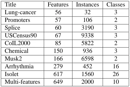
5.3.1 UCIBENCHMARK DATA
Title Features Instances Classes
Lung-cancer 56 32 3
Promoters 57 106 2
Splice 60 3190 3
USCensus90 67 9338 3
CoIL2000 85 5822 2
Chemical 150 936 3
Musk2 166 6598 2
Arrhythmia 279 452 16
Isolet 617 1560 26
Multi-features 649 2000 10
Table 2: Summary of UCI benchmark data sets.
All together 10 data sets in the traditional form are selected from the UCI Machine Learning Repository1and the UCI KDD Archive.2 These data sets contain various numbers of features, in-stances, and classes, as shown in Table 2. For each data set, we first run all the feature selection
rithms in comparison, and obtain the running time and selected features for each algorithm. For data sets containing features with continuous values, we apply the MDL discretization method (Fayyad and Irani, 1993) before applying FCBF, CFS-SF, and FOCUS-SF. For ReliefF, we use 5 neigh-bors and 30 instances throughout the experiments as suggested by Robnik-Sikonja and Kononenko (2003). We then apply NBC and C4.5 on both the original data set and each of the newly obtained data sets (with only selected features), and obtain overall accuracy of 10-fold cross-validation. All experiments were conducted on a Pentium IV PC with 1 GB RAM.
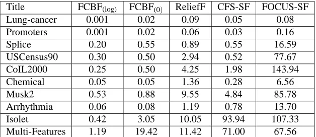
Table 3 records the running time for each feature selection algorithm. We can observe that FCBF(0) is consistently faster than CFS-SF and FOCUS-SF. The time savings from FCBF(0) be-come more obvious when the data dimensionality increases. In many cases especially compared with FOCUS-SF, the time savings are in degrees of magnitude. These results verify the superior computational efficiency of sequential forward selection with elimination applied by FCBF over greedy sequential search applied by CFS-SF and FOCUS-SF. Comparison between FCBF(0) and
ReliefF shows that ReliefF is unexpectedly slow even though its time complexity is linear to di-mensionality. The reason lies in that searching for nearest neighbors in ReliefF involves distance calculation which is more costly than the calculation of symmetrical uncertainty. When we compare FCBF(0)with FCBF(log), it is clear that the setting of a larger relevance thresholdγfurther speeds up FCBF.
Title FCBF(log) FCBF(0) ReliefF CFS-SF FOCUS-SF
Lung-cancer 0.001 0.02 0.09 0.05 0.08
Promoters 0.001 0.02 0.06 0.03 0.16
Splice 0.20 0.55 0.89 0.55 16.59
USCensus90 0.30 0.50 2.94 0.52 77.67
CoIL2000 0.25 0.50 4.25 1.98 143.94
Chemical 0.05 0.05 1.36 0.28 6.56
Musk2 0.53 0.88 9.55 4.84 85.78
Arrhythmia 0.06 0.08 1.19 0.78 13.70
Isolet 0.42 3.05 10.05 93.94 107.33
Multi-Features 1.19 19.42 11.42 71.00 67.56
Table 3: Running time (seconds) for each feature selection algorithm on UCI data.
Table 4 records the number of features selected by each feature selection algorithm. We can see that all these algorithms achieve significant reduction of dimensionality by selecting only a small portion of the original features. FCBF(log)on average selects the smallest number of features.
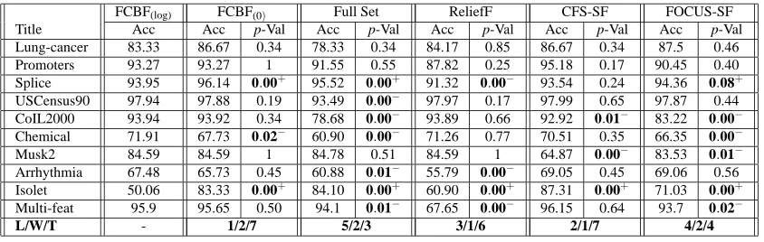
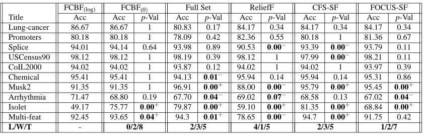
Tables 5 and 6 show the 10-fold cross-validation accuracy of NBC and C4.5 respectively. For each data set, we conduct Student’s paired two-tailed t-Test in order to evaluate the statistical sig-nificance of the difference between two averaged accuracy values: one resulted from FCBF(log)and the other resulted from one of FCBF(0), the full set, ReliefF, CFS-SF, and FOCUS-SF. Each value
in a p-val column records the probability associated with the t-Test. The smaller the value, the more significant the difference of the two average values is. The last row (L/W/T) in each table summa-rizes over all data sets the losses/wins/ties in accuracy (at significance level 0.1) comparing various feature sets with those selected by FCBF(log). We can see that in general FCBF(log)achieves similar accuracy as FCBF(0). Therefore, the effectiveness of FCBF can be verified from the following two
Title FCBF(log) FCBF(0) ReliefF CFS-SF FOCUS-SF
Lung-cancer 4 6 5 8 4
Promoters 6 6 4 4 4
Splice 9 22 11 6 10
USCensus90 3 4 2 1 13
CoIL2000 3 5 12 10 29
Chemical 4 5 7 7 11
Musk2 2 2 2 10 11
Arrhythmia 5 12 25 25 24
Isolet 5 32 23 137 11
Multi-Features 27 130 14 87 7
Average 7 22 11 30 12
Table 4: Number of features selected by each feature selection algorithm on UCI data.
FCBF(log) FCBF(0) Full Set ReliefF CFS-SF FOCUS-SF
Title Acc Acc p-Val Acc p-Val Acc p-Val Acc p-Val Acc p-Val
Lung-cancer 83.33 86.67 0.34 78.33 0.34 84.17 0.85 86.67 0.34 87.5 0.46 Promoters 93.27 93.27 1 91.55 0.55 87.82 0.25 95.18 0.17 90.45 0.40 Splice 93.95 96.14 0.00+ 95.52 0.00+ 91.32 0.00− 93.54 0.24 94.36 0.08+
USCensus90 97.94 97.88 0.19 93.49 0.00− 97.97 0.17 97.99 0.65 97.87 0.44 CoIL2000 93.94 93.92 0.34 78.68 0.00− 93.89 0.66 92.92 0.01− 83.22 0.00−
Chemical 71.91 67.73 0.02− 60.90 0.00− 71.26 0.77 70.51 0.35 66.35 0.00−
Musk2 84.59 84.59 1 84.78 0.51 84.59 1 64.87 0.00− 83.53 0.01−
Arrhythmia 67.48 65.73 0.45 60.88 0.01− 55.79 0.00− 69.05 0.45 69.06 0.56 Isolet 50.06 83.33 0.00+ 84.10 0.00+ 60.90 0.00+ 87.31 0.00+ 71.03 0.00+
Multi-feat 95.9 95.65 0.50 94.1 0.01− 67.65 0.00− 96.15 0.64 93.7 0.02−
L/W/T - 1/2/7 5/2/3 3/1/6 2/1/7 4/2/4
Table 5: Accuracy of NBC on selected features for UCI data: Acc records 10-fold cross-validation accuracy rate(%)and p-Val records the probability associated with a paired two-tailed t-Test. The symbols “+” and “−” respectively identify statistically significant (at 0.1 level) wins or losses over FCBF(log).
improvement is more pronounced for NBC; and (2) FCBF(log) can achieve similar or even higher accuracy compared with other algorithms.
5.3.2 NIPSBENCHMARK DATA
Three data sets with very high dimensionality but relatively few instances are selected from the NIPS 2003 feature selection benchmark data sets.3 All these data sets contain two classes and a large number of artificially introduced random features in addition to real features. A summary of the data sets is given in Table 7. For each data set, we conduct experiments following the same procedure as that used in UCI data. The results are shown in Tables 8, 9, 10, and 11.
From Table 8, we observe similar trends as those from UCI data except that (1) for Dexter and Dorothea data, CFS-SF did not produce running time results (hence, neither selected features nor
FCBF(log) FCBF(0) Full Set ReliefF CFS-SF FOCUS-SF
Title Acc Acc p-Val Acc p-Val Acc p-Val Acc p-Val Acc p-Val
Lung-cancer 86.67 86.67 1 80.83 0.17 84.17 0.34 84.17 0.34 84.17 0.34 Promoters 80.18 80.18 1 78.09 0.42 82.36 0.55 80.18 1 81.36 0.67 Splice 94.01 94.14 0.64 93.98 0.89 90.53 0.00− 93.39 0.00− 93.79 0.11 USCensus90 98.12 98.12 1 98.19 0.39 98.12 1 97.99 0.00− 98.21 0.11 CoIL2000 94.02 94.02 1 93.87 0.12 94.02 1 94.02 1 93.97 0.39 Chemical 95.41 95.41 1 94.13 0.01− 95.94 0.14 95.94 0.14 95.31 0.86 Musk2 91.35 91.35 1 96.91 0.00+ 88.00 0.00− 95.79 0.00+ 95.45 0.00+
Arrhythmia 71.47 68.80 0.19 67.70 0.04− 69.02 0.07− 68.58 0.13 67.02 0.04−
Isolet 49.17 75.77 0.00+ 79.87 0.00+ 59.10 0.00+ 81.35 0.00+ 68.84 0.00+
Multi-feat 92.45 93.65 0.04+ 94.3 0.01+ 78.65 0.00− 94.7 0.00+ 91.75 0.42
L/W/T - 0/2/8 2/3/5 4/1/5 2/3/5 1/2/7
Table 6: Accuracy of C4.5 on selected features for UCI data: Acc records 10-fold cross-validation accuracy rate(%)and p-Val records the probability associated with a paired two-tailed t-Test. The symbols “+” and “−” respectively identify statistically significant (at 0.1 level) wins or losses over FCBF(log).
Features Instances
Title Total Real Random Total Class 1 Class 2
Arcene 10000 7000 3000 100 44 56
Dexter 20000 9947 10053 300 150 150
Dorothea 100000 50000 50000 800 78 722
Table 7: Summary of NIPS benchmark data sets.
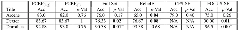
accuracy results) because the program ran out of memory after a period of considerably long time due to its quadratic space complexity; and (2) FCBF achieves tremendous time savings for this group of data sets, for instance, roughly 1 minute by FCBF(log) versus 4.5 hours by FOCUS-SF in Dorothea data. Results in Table 9 show that all the algorithms in comparison can dramatically reduce the dimensionality for this group of data sets. In spite of its impressive efficiency and capability of dimensionality reduction, the effectiveness of FCBF can still be clearly revealed by the results in Tables 10 and 11. As we can see, FCBF either improves or maintains the accuracy of both NBC and C4.5 for all the three data sets. In addition, for each of the three data sets, the highest accuracy is achieved by applying NBC on the feature subset selected by FCBF.
Title FCBF(log) FCBF(0) ReliefF CFS-SF FOCUS-SF
Arcene 0.42 0.75 9.16 1108.66 21.39
Dexter 1.80 2.63 45.43 N/A 928.78
Dorothea 68.95 393.80 349.27 N/A 16470.92
Title FCBF(log) FCBF0 ReliefF CFS-SF FOCUS-SF
Arcene 24 39 45 50 4
Dexter 35 35 71 N/A 23
Dorothea 50 96 137 N/A 21
Table 9: Number of features selected by each feature selection algorithm on NIPS data.
FCBF(log) FCBF(0) Full Set ReliefF CFS-SF FOCUS-SF
Title Acc Acc p-Val Acc p-Val Acc p-Val Acc p-Val Acc p-Val
Arcene 91.0 93.0 0.34 69.0 0.00− 69.0 0.02− 92.0 0.68 59.0 0.00−
Dexter 90.0 90.0 1 88.0 0.26 73.00 0.00− N/A N/A 90.0 1 Dorothea 97.5 98.38 0.01+ 90.25 0.00− 94.38 0.00− N/A N/A 95.25 0.00−
Table 10: Accuracy of NBC on selected features for NIPS data: Acc records 10-fold cross-validation accuracy rate(%)and p-Val records the probability associated with a paired two-tailed t-Test. The symbols “+” and “−” respectively identify statistically significant (at 0.1 level) wins or losses over FCBF(log).
5.4 Summary
From the previous empirical study, we can conclude that FCBF can efficiently achieve high degree of dimensionality reduction and enhance or maintain predictive accuracy with selected features. Its proven efficiency and effectiveness compared with other algorithms through various synthetic and benchmark data sets suggest that FCBF is practical for feature selection of high-dimensional data. It is worthy to emphasize that feature subsets selected by FCBF are decoupled from the choice of learning algorithms. In other words, FCBF does not directly aim to increase the accuracy of a particular learning algorithm as wrapper algorithms do. In order to achieve better accuracy within affordable time, a wrapper algorithm based on an intended learning algorithm can be applied to the significantly reduced subset obtained from FCBF.
In FCBF, there is one parameter, the relevance threshold γ. As consistently shown from the benchmark data, different settings ofγaffect the speed of FCBF. The closerγis set to 1, the faster FCBF is. As shown from Corral-47 and Corral-46 as well as many of the benchmark data sets which may contain a large number of irrelevant and/or redundant features, speeding up the algorithm by
FCBF(log) FCBF(0) Full Set ReliefF CFS-SF FOCUS-SF
Title Acc Acc p-Val Acc p-Val Acc p-Val Acc p-Val Acc p-Val
Arcene 83.0 82.0 0.76 76.0 0.17 65.0 0.04− 79.0 0.40 75.0 0.26 Dexter 83.67 83.67 1 76.33 0.02− 76.67 0.08− N/A N/A 90.00 0.01+
Dorothea 92.88 93.0 0.76 90.38 0.01− 93.38 0.68 N/A N/A 96.5 0.00+
settingγto a reasonably large value does not sacrifice the goodness of the selected subsets. However, a close look at the accuracy of individual data sets in Tables 5 and 6 reveals that in certain cases (e.g., Isolet data), FCBF(log)results in significantly reduced accuracy than FCBF(0)due to the setting
of overly high threshold. Therefore, when we do not have prior knowledge about data, an easy and safe way of applying FCBF is to setγto the default value 0.
6. Conclusions
In this paper, we have identified the need for explicit redundancy analysis in feature selection, provided a formal definition of feature redundancy, and investigated the relationship between feature relevance and redundancy. We have proposed a new framework of efficient feature selection via relevance and redundancy analysis, and a correlation-based method which uses C-correlation for relevance analysis and both C- and F-correlations for redundancy analysis. A new feature selection algorithm FCBF is implemented and evaluated through extensive experiments comparing with three representative feature selection algorithms. The feature selection results are further verified by two different learning algorithms. Our method demonstrates its efficiency and effectiveness for feature selection in supervised learning in domains where data contains many irrelevant and/or redundant features.
Some future works are planed along the following directions. First, since symmetrical uncer-tainty measure only handles nominal or discrete values, our current method requires continuous values be discretized, which opens the opportunity to investigate how different discretization meth-ods affect the performance of FCBF. Second, it would be interesting to explore measures that can handle all types of values or ways of combining different measures under our framework of rele-vance and redundancy analysis. Another direction is to investigate how our method can be extended to deal with regression problems in which the class contains continuous values. Moreover, addi-tional effort is needed to experiment our method on genomic microarray data for informative gene selection and investigate how small samples affect the performance of feature selection.
Acknowledgments
We gratefully thank the Action Editor and anonymous reviewers for their constructive comments. This work is in part supported by the National Science Foundation (NSF grant No. 0127815, 0231448) and Prop 301 (No. ECR A601) at ASU.
References
H. Almuallim and T. G. Dietterich. Learning boolean concepts in the presence of many irrelevant features. Artificial Intelligence, 69(1-2):279–305, 1994.
D. A. Bell and H. Wang. A formalism for relevance and its application in feature subset selection.
Machine Learning, 41(2):175–195, 2000.
A. L. Blum and P. Langley. Selection of relevant features and examples in machine learning.
A. L. Blum and R. L. Rivest. Training a 3-node neural networks is NP-complete. Neural Networks, 5:117 – 127, 1992.
M. Dash, K. Choi, P. Scheuermann, and H. Liu. Feature selection for clustering – a filter solution. In Proceedings of the Second International Conference on Data Mining, pages 115–122, 2002.
M. Dash and H. Liu. Feature selection for classification. Intelligent Data Analysis: An International
Journal, 1(3):131–156, 1997.
M. Dash and H. Liu. Consistency-based search in feature selection. Artificial Intelligence, 151(1-2): 155–176, 2003.
J. G. Dy, C. E. Brodley, A. C. Kak, L. S. Broderick, and A. M. Aisen. Unsupervised feature selection applied to content-based retrieval of lung images. IEEE Transactions on Pattern Analysis and
Machine Intelligence, 25(3):373–378, 2003.
U. M. Fayyad and K. B. Irani. Multi-interval discretization of continuous-valued attributes for clas-sification learning. In Proceedings of the Thirteenth International Joint Conference on Artificial
Intelligence, pages 1022–1027, 1993.
G. Forman. An extensive empirical study of feature selection metrics for text classification. Journal
of Machine Learning Research, 3:1289–1305, 2003.
I. Guyon and A. Elisseeff. An introduction to variable and feature selection. Journal of Machine
Learning Research, 3:1157–1182, 2003.
M. A. Hall. Correlation-based feature selection for discrete and numeric class machine learning. In
Proceedings of the Seventeenth International Conference on Machine Learning, pages 359–366,
2000.
T. Hastie, R. Tibshirani, and J. Friedman. The Elements of Statistical Learning. Springer, 2001.
D. D. Jensen and P. R. Cohen. Multiple comparisions in induction algorithms. Machine Learning, 38(3):309–338, 2000.
G. H. John, R. Kohavi, and K. Pfleger. Irrelevant feature and the subset selection problem. In
Proceedings of the Eleventh International Conference on Machine Learning, pages 121–129,
1994.
Y. Kim, W. Street, and F. Menczer. Feature selection for unsupervised learning via evolutionary search. In Proceedings of the Sixth ACM SIGKDD International Conference on Knowledge
Dis-covery and Data Mining, pages 365–369, 2000.
R. Kohavi and G. H. John. Wrappers for feature subset selection. Artificial Intelligence, 97(1-2): 273–324, 1997.
D. Koller and M. Sahami. Toward optimal feature selection. In Proceedings of the Thirteenth
International Conference on Machine Learning, pages 284–292, 1996.
W. Lee, S. J. Stolfo, and K. W. Mok. Adaptive intrusion detection: A data mining approach. AI
H. Liu, F. Hussain, C. L. Tan, and M. Dash. Discretization: An enabling technique. Data Mining
and Knowledge Discovery, 6(4):393–423, 2002a.
H. Liu and H. Motoda. Feature Selection for Knowledge Discovery and Data Mining. Boston: Kluwer Academic Publishers, 1998. ISBN 0-7923-8198-X.
H. Liu, H. Motoda, and L. Yu. Feature selection with selective sampling. In Proceedings of the
Nineteenth International Conference on Machine Learning, pages 395–402, 2002b.
H. Liu and R. Setiono. A probabilistic approach to feature selection - a filter solution. In Proceedings
of the Thirteenth International Conference on Machine Learning, pages 319–327, 1996.
A. Miller. Subset Selection in Regression. Chapman & Hall/CRC, 2 edition, 2002.
T. M. Mitchell. Machine Learning. McGraw-Hill, 1997.
P. Mitra, C. A. Murthy, and S. K. Pal. Unsupervised feature selection using feature similarity. IEEE
Transactions on Pattern Analysis and Machine Intelligence, 24(3):301–312, 2002.
K. S. Ng and H. Liu. Customer retention via data mining. AI Review, 14(6):569 – 590, 2000.
W. H. Press, S. A. Teukolsky, W. T. Vetterling, and B. P. Flannery. Numerical Recipes in C. Cam-bridge University Press, CamCam-bridge, 1988.
J. R. Quinlan. C4.5: Programs for Machine Learning. Morgan Kaufmann, 1993.
M. Robnik-Sikonja and I. Kononenko. Theoretical and empirical analysis of Relief and ReliefF.
Machine Learning, 53:23–69, 2003.
D. L. Swets and J. J. Weng. Efficient content-based image retrieval using automatic feature selection. In IEEE International Symposium on Computer Vision, pages 85–90, 1995.
I. H. Witten and E. Frank. Data Mining - Pracitcal Machine Learning Tools and Techniques with
JAVA Implementations. Morgan Kaufmann Publishers, 2000.
E. Xing, M. Jordan, and R. Karp. Feature selection for high-dimensional genomic microarray data. In Proceedings of the Eighteenth International Conference on Machine Learning, pages 601–608, 2001.
Y. Yang and J. O. Pederson. A comparative study on feature selection in text categorization. In
Proceedings of the Fourteenth International Conference on Machine Learning, pages 412–420,
1997.
L. Yu and H. Liu. Feature selection for high-dimensional data: a fast correlation-based filter so-lution. In Proceedings of the twentieth International Conference on Machine Learning, pages 856–863, 2003.
L. Yu and H. Liu. Redundancy based feature selection for microarray data. In Proceedings of the
Tenth ACM SIGKDD Conference on Knowledge Discovery and Data Mining, pages 737–742,