Mathematical Study on MHD Squeeze Flow between Two Parallel Disks with Suction or Injection via HAM and HPM and Its Applications

Mathematical Study on MHD Squeeze Flow

between Two Parallel Disks with Suction or

Injection via HAM and HPM and Its

Applications

Anil Kumar#1, S P Agrawal*2

#1

Department of Applied Sciences (Mathematics) Chandigarh Engineering College, Landran Mohali Punjab India #2

Department of Civil Engineering, Sai Nath University Ranchi, Jharkhand India

Abstract-In this paper, we are considering the problem of magneto-hydrodynamic MHD squeeze flow of an electrically conducting fluid between two infinite, parallel disks are investigated. The analytical method called Homotopy Analysis Method (HAM) and Homotopy Perturbation Method (HPM) are used to compute an approximation for the solution of nonlinear differential equations governing on the problem. The results of the mentioned methods are compared with a type of numerical analysis as Boundary Value Problem method.

Keywords — Magneto-hydrodynamic Homotopy

Perturbation Method, Squeeze flow, Temprature , nonlinear differential equations, incompressible flow.

I. INTRODUCTION

The application of a MHD fluid in lubrication prevents the adverse impact of temperature on the fluid viscosity when the system operates under boundary conditions. The problem considered is of general interest in the theory of magneto-hydrodynamic lubrication and other related applications. In particular, the results of the present investigation are directly applicable to the hydrodynamics of high temperature bearings lubricated with liquid metals. A number of theoretical and experimental investigations into magneto-hydrodynamic effects in lubrication have been reported. These include among other works of Hughes and Elco [1], Kuzma et al. [2] and Krieger et al. [3]. Most scientific problems such as two-dimensional viscous flow between slowly expanding or contracting walls with weak permeability and other fluid mechanic problems are inherently nonlinear. In most cases, these problems do not admit analytical solution, so these equations should be solved using special techniques. In recent years, much attention has been devoted to the newly developed methods to construct an analytic solution of equation such as the method included the Perturbation techniques. Perturbation techniques are too strongly dependent upon the so-called ‘‘small

parameters’’ [4]. Other different methods have introduced to solve nonlinear equations such as the δ-expansion method [5], Adomian’s decomposition method [6], Homotopy Perturbation Method (HPM) [7–10], Variational Iteration Method (VIM) [11–14], Homotopy analysis method [15-18], Optimal Homotopy Asymptopic Method (OHAM)[19,20] and optimal Homotopy Perturbation Method (OHPM)[21]. In this letter, analytical solutions of nonlinear equations arising of magneto-hydrodynamic MHD squeeze flow of an electrically conducting fluid between two infinite, parallel disks have been studied by the two analytical methods. These methods called Homotopy Analysis Method (HAM), Homotopy Perturbation Method (HPM) do not have small parameters. Obtaining the analytical solution of the models and comparing with the numerical result reveal the capability, effectiveness and convenience of HAM and HPM. These methods give successive approximations of high accuracy solution. Kumar et al. [23]investigated a finite difference technique for reliable MHD steady flow through channels permeable boundaries.Kumaret al [24] investigated MHD free convective fluctuating flow through a porous effect with variable permeability Parameter.Kumar et al. [25] investigated mathematical analysis of MHD on laminar mixed convection of newtonian fluid between vertical parallel plates channel. Kumar et al. [26] investigated a Crank-Nicholson scheme to transient MHD free convective flow through semi-infinite vertical porous plate with constant suction and temperature dependent heat source.

II. MATHEMATICALMODEL

In the present investigation, consider an axi-symmetric incompressible flow between two parallel infinite disks, which at time

t

*, are space a distance





1

* ₂

1

proportional to





1 * ₂ 0

1

B



a t

 is applied perpendicularly to the disks [6, 22]. The upper disk at





1 * 2

1

z



H



a t

is moving with velocity





1

* ₂

1

1

2



H

a t







towards the stationary lower

disk at

z



0

. The axial coordinate is denoted by

z

*

and the radial coordinate by

r

*. With the axial and radial velocities denoted by

w

* and

u

*, respectively, we introduce the following quantities:

 

 

 

*

* * 0

* _{* *}

*

* *

*

,

,

2 1

₁

₁

,

,

1

B

r

H

u

f

w

f

B

at

_at

_at

z

r r

t t

H

at



_



_













_

_









(1)

The equation of continuity is satisfied and the momentum equations are reduced to:





2

( ) ( ) 3 ( ) 2 ( ) ( ) ( ) 0

f S f  f  f f M f  (2)

Where * 1

1

( )

p

p t

r

r



_



has been used,

2

2

H

S







and 2 0

B

M







that



denotes density,



denotes kinetic viscosity and



denotes fluid electrical conductivity. The boundary conditions are given by:

1

(0)

,

(0) 0,

(1)

,

(1) 0

2

f



A

f





f



f





(3) Where,

A

is the constant parameter such that

0

A



corresponds to suction and

A



0

to injection.

III. APPLICATIONOFHOMOTOPY

ANALYSISMETHOD

For HAM solutions, we choose the initial guess and auxiliary linear operator in the following form:

  



3 2

0

3

1 2 3 ,

2

f     A  _  A_ A

 

(4)

( )

,

L f



f



(5)

3 2

1 2 3 4

1

1

(

)

0,

6

2

L

c y



c y



c y



c



(6)

Where

c i

i

(



1, 2, 3, 4)

are constant. Let

 

0

,

1



P

denotes the embedding parameter and



indicates non –zero auxiliary parameters.

Zeroth –order deformation equations

(1



P L F

)



( ; )



p



f

₀

( )







p H



( )



N F



( ; )



p



(7)

1

(0; ) ; (0; ) 0, (1; ) , (1; ) 0

2

F p A F p  F p  F p  (8)

2

4 3 2 2

4 3 2 2

3 2

3 2

( ; ) ( ; ) ( ; ) ( ; )

[ ( ; )] 3

( ; ) ( ; ) ( ; ) ( ; )

2

d F p d F p d F p d F p

N F p S

d d d d

d F p dF p d F p F p d d d M S                                    (9)

For

p



0

and

p



1

we have

0

( ;0)

( )

( ;1)

( )

F





f



F





f



(10)

When p increases from 0 to 1 then

F

( ; )



p

varies from

f

0

( )



to

f

( )



. By Taylor's theorem and

using Eq. (9),

F

( ; )



p

can be expanded in a power series of p as follows:

0

1 ₀

1 ( ( ; ))

( ; ) ( ) ( ) , ( )

! m m

m m m

m _p

F p

F p f f p f

m p             



(11)

In which



is chosen in such a way that this series is convergent at

p



1

, therefore we have in according to Eq. (10) that

0

1

( )

( )

m

( ),

m

f



f



f













(12)

mth –order deformation equations



m( ) m m1( )



( ) m( )

L f   f_  H R  (13)

(0; ) 0; (0; ) 0, (1; ) 0, (1; ) 0

F p F p F p  F p  (14)

 

2 1

1 1 1 1 1

0

3 2

m

m m m m m m k k

k

R  f S f f M f S f f



     



   

  

  _  _ 



(15)

Now we determine the convergence of the result, the differential equation, and the auxiliary function according to the solution expression. So, let us assume:

( ) 1

H





(16)

     

   

7 6

1

2 5 2 4

2 2 2 3

2 2 2

1 1 1 1

3 1 2 3 1 2

210 105 30 60

1 1 1 1 1

3 1 2 3 1 2

60 15 24 6 8

13 39 1 52 1 5 19 70 140 10 35 5 28 280 1 22 1

40 35 20

f A S S A A S A S

A M S A M SA S

S A S M S A M A S A S

M S A M A

              _  _    _  _            _  _    _   _         _     _  _               2    (17)

The solutions

f

( )



were too long to be mentioned here, therefore they are shown graphically.

IV. APPLICATION OF HOMOTOPY PERTURBATION

METHOD

In this section, we employ HPM to solve Eq. (2 ) subject to boundary conditions Eq.(3).We can construct Homotopy function of Eq. (2) as described in [22]:

       



 



2

0

, 1 ( ) ( ) 3 ( ) 2 ( ) ( )

( ) 0,

H f p P f g y p f S f f f f

M f                            , (18)

Where

p



_

0 ,1

_ is an embedding parameter. For

0

p



and

p



1

we have:

   

,0

0

,

   

,1

f





f



f





f



(19) Note that when p increases from 0 to 1,



,



f



p

varies from

f

₀

 



to

f

 



.By substituting:

 

   

2

 

 

0 1 2 0

0 , 0

n i

i i

f f  p f  p f  p f  g



     (20)

From equation (33) and rearranging the result based on powers of p-terms, we get:

 

0

0

0 0 0 0

: ( ) 0

1

(0) ; 0 0, (1) , (1) 0

2

P f

f A f f f

  

 

    (21)

 

 

     

 

 

 

 

   

1 2

1 0 0 0 0 0

1 1 1 1

: 2 3 0

(0) 0; 0 0, (1) 0, (1) 0

P f S f Sf f S f M f

f f f f

                       (22)      

 

 

     

 

 

   

 

  2

2 1 0 1 0 1 1

2 1

2 2 2 2

: 2 3 2

0

(0) 0; 0 0, (1) 0, (1) 0

P f S f f S f Sf f S f

M f

f f f f

                           (23)

 

 

 

 

 

   

 

   

 

   

 

 

 

 

3 2

3 2 2 0 2 2 0

1 1 2

3 3 3 3

: 3 2 2

2 0

(0) 0; 0 0, (1) 0, (1) 0

P f S f M f Sf f Sf f

Sf f S f

f f f f

                               (24)

Solving Esq. (21) – (24) with boundary conditions, we have (for example

S



0.1,

M



2

,

A



1

):

 

3 2

0

1.500000000

1,

f

 









(25)

 

7 6 5 4 1

3 2

0.001428571429 0.0050000 0.180000 0.4125000 0.2978571429 0.06178571429

f     

 

   

  ,

(26)

  11 10 9

2

8 7 6 5

4 3 2

0.000007792207792 0.00004285714286 0.0009087301587 0.0036607142 0.0188153061 0.043820238 0.03711428571 0.004157738100 0.005947057248 0.0007824906815

f    

                 (27)

 

8 15 7 14 6 13

3

12 11 10

9 8 7

6

4.99976214310 3.74982160710 0.692501942410

0.000038502886 0.0002321360544 0.0008178911564

0.0019451346370 0.0030426296780 0.002043508165

0.0007230726130 0.001236779

f    

                  

  5 4

3 2 829 0.00005608490221 0.0001191218468 0.0001223151002        (28)

The solution of this equation, when

p



1

, will be as follows:

 

3

 

0 1

i i i p

f



Lim p f



 

 

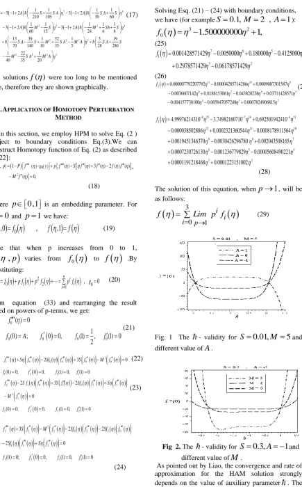
(29)

Fig. 1 The



- validity for

S



0.01,

M



5

and different value of

A

.

Fig 2. The



- validity for

S



0.3,

A

 

1

and different value of

M

.

auxiliary parameter



provides us with a convenient way to adjust and control the convergency. The range of



for convergency is obtained according to figs. 1 and 2. For

S



0.01,

M



5

and

7

A

7

  

the ranges



0.4

  



1.5

, for

0.3,

1

S



A

 

and

0



M



5

the ranges



0.5

  



1.3

, give suitable value of



for convergency. Then,



 

0.9

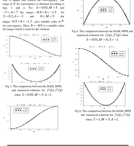
is a suitable value for ranges which is used for the solution.

Fig 3. The comparison between the HAM, HPM and numerical solutions for

f

( ),



f



( )



when

S



0.01,

M



5,

A



1

. .

Fig 4. The comparison between the HAM, HPM and numerical solutions for

f

( ),



f



( )



when

0.01,

0,

1

S



M



A

 

.

Fig 6. The comparison between the HAM, HPM and numerical solutions for

f

( ),



f



( )



when

S



1,

M



3,

A



1

.

Table 1 The results of HAM, HPM and Numerical methods for

f

 



when

0.4,

2,

1

S



M



A



0.45 0.792606371 0.792606388 0.792606372 0.0000000010 0.0000000150 0.50 0.755635547 0.755635562 0.755635547 0.0000000005 0.0000000150 0.55 0.718443074 0.718443087 0.718443074 0.0000000008 0.0000000130 0.60 0.681750643 0.681750657 0.681750644 0.0000000013 0.0000000130 0.65 0.646296385 0.646296395 0.646296386 0.0000000005 0.0000000094 0.70 0.612838519 0.612838521 0.612838518 0.0000000014 0.0000000034 0.75 0.582159131 0.582159137 0.582159133 0.0000000014 0.0000000041 0.80 0.555068148 0.555068152 0.555068148 0.0000000001 0.0000000040 0.85 0.532407454 0.532407455 0.532407454 0.0000000006 0.0000000008 0.90 0.515055312 0.515055311 0.515055310 0.0000000013 0.0000000004 0.95 0.503931027 0.503931026 0.503931027 0.0000000001 0.0000000002 1.00 0.499999999 0.499999997 0.500000000 0.0000000012 0.0000000026

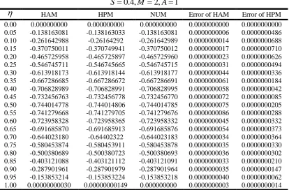
Table 2 The results of HAM, HPM and Numerical methods for

f



 



when

0.4,

2,

1

S



M



A





HAM HPM NUM Error of HAM Error of HPM 0.00 0.000000000 0.000000000 0.000000000 0.0000000000 0.0000000000 0.05 -0.138163081 -0.138163033 -0.138163081 0.0000000006 0.0000000486 0.10 -0.261642988 -0.26164292 -0.261642989 0.0000000014 0.0000000688 0.15 -0.370750011 -0.370749941 -0.370750012 0.0000000017 0.0000000710 0.20 -0.465725958 -0.465725897 -0.465725960 0.0000000023 0.0000000626 0.25 -0.546745711 -0.546745665 -0.546745715 0.0000000031 0.0000000494 0.30 -0.613918173 -0.613918144 -0.613918177 0.0000000044 0.0000000336 0.35 -0.667286685 -0.667286672 -0.667286691 0.0000000061 0.0000000184 0.40 -0.706828989 -0.706828991 -0.706828995 0.0000000058 0.0000000042 0.45 -0.732456763 -0.732456778 -0.732456770 0.0000000072 0.0000000085 0.50 -0.744014778 -0.744014806 -0.744014785 0.0000000075 0.0000000205 0.55 -0.741279668 -0.741279705 -0.741279676 0.0000000086 0.0000000288 0.60 -0.723958328 -0.723958365 -0.723958332 0.0000000045 0.0000000332 0.65 -0.691685870 -0.691685913 -0.691685876 0.0000000054 0.0000000373 0.70 -0.644023180 -0.64402322 -0.644023183 0.0000000034 0.0000000364 0.75 -0.580453874 -0.580453911 -0.580453878 0.0000000035 0.0000000330 0.80 -0.500380689 -0.500380723 -0.500380693 0.0000000036 0.0000000302 0.85 -0.403121088 -0.403121112 -0.403121091 0.0000000033 0.0000000210 0.90 -0.287901961 -0.287901979 -0.287901964 0.0000000035 0.0000000147 0.95 -0.153853214 -0.153853224 -0.153853218 0.0000000040 0.0000000062 1.00 0.00000000030 0.00000000149 0.000000000 0.0000000003 0.0000000014

In this study, the problem of magneto-hydrodynamic MHD squeeze flow of an electrically conducting fluid between two infinite, parallel disks was analyzed using HAM and HPM. By the drawing of 2-D fig. 3 to 6, of the numerical solution, HPM and HAM solutions for f y( ) and f( )y with different values of

S M

,

and

A

, we see that the Homotopy Analysis Method and Homotopy Perturbation Method are more accurate than NUM. According to fig. 3 to 6 and tables 1 and 2 these methods provide highly accurate analytic solutions for nonlinear problems in comparison with the numerical solution. The comparison of the method reveals that the approximations obtained by HAM and HPM converge to the exact solution quite fast. Also, the

auxiliary parameter



provides us with a convenient way to adjust and control the convergence and its rate for the solutions series. Finally, it has been attempted to show the capabilities and wide-range applications of the HAM and HPM in comparison with the numerical solution of nonlinear equations.

7. CONCLUSION

They offer superior accuracy in comparison with the NUM. Also, it is found that these methods are powerful mathematical tools and that they can be applied to a large class of linear and nonlinear problems arising in different fields of science and engineering specially some heat transfer equations.

Acknowledgment

Author is grateful to Chandigarh Engineering college Landran Mohali, India for providing facilities and encouragement to complete this work. Also, the corresponding authors are thankful to the learned referees for their fruitful suggestions for improving the presentation of this work. The author would like to thanks Smt. Namita Varshney, Ridansh and Siddika for providing emotional happiness during this research work.

REFERENCES

[1] Hughes, W. F., Elco, R. A., Magnetohydrodynamic lubrication flow between parallel rotating disks, Journal of Fluid Mechanics, 13 (1962), 1, pp. 21–32.

[2] kuzma, D. C., Maki, E. R., Donnelly, R. J., The magneto hydrodynamic squeeze film,” Journal of Fluid Mechanics, 19(1964), 3, pp. 395–400.

[3] Krieger, R. J., Day, H. J., Hughes, W. F., The MHD hydrostatics thrust bearings—theory and experiments, ASME Journal of Lubrication Technology, 89(1967), pp. 307–313.

[4] Nayfeh, A.H., Perturbation Methods, Wiley, New York, USA, 2000.

[5] Ganji, D.D., Hashemi Kachapi, Seyed H., Analytical and numerical method in Engineering and applied Science, progress in nonlinear science, 3(2011), pp.1-579.

[6] Ganji, D.D., Hashemi Kachapi, Seyed H., Analysis of nonlinear Equations in fluids, progress in nonlinear science, 3 (2011), pp.1-294.

[7] He, J.H., Homotopy perturbation method for bifurcation of nonlinear problems, Int. J. Nonlinear Sci. Numer. Simul, 6(2005), pp. 207-208.

[8] He, J.H., Application of homotopy perturbation method to nonlinear wave equations, Chaos Solitons Fractals, 26(2005),pp. 695-700.

[9] He, J. H., Homotopy perturbation technique, Comp. Meth. App. Mech. Eng., 178 (1999), pp. 257-262.

[10] Rostamiyan, Y., Ganji, D. D., Rahimi Petroudi, I., KhazayiNejad, M., analytical investigation of nonlinear model arising in heat transfer through the porous film , THERMAL SCIENCE,(in press).

[11] Ganji, D.D., Sadighi, A., Application of homotopy-perturbation and variational iteration methods to nonlinear heat transfer and porous media equations, J. Comput. Appl. Math,207 (2007),1,pp. 24-34.

[12] He, J.H., Variational iteration method – some recent results and new interpretations, Journal of Computational and Applied Mathematics, 207 (2007), 1, pp. 3–17.

[13] Momani,S ., Abuasad ,S., Application of He’s variational iteration method to Helmholtz equation, Chaos Solitons & Fractals, 27 (2006),5,pp. 1119–1123.

[14] Ganji, D.D., Afrouzi, G.A., Talarposhti, R.A., Application of variational iteration method and homotopy-perturbation method for nonlinear heat diffusion and heat transfer equations, Physics Letters A, 368(2007),pp. 450–457. [15] Liao SJ. Boundary element method for general nonlinear

differential operators, Eng Anal Bound Elem, 202(1997), pp. 91–9.

[16] Liao SJ., Cheung KF. Homotopy analysis of nonlinear progressive waves in deep water. J Eng Math,45(2003), 2, pp. 103–16.

[17] Liao SJ., On the homotopy analysis method for nonlinear problems. Appl Math Comput, 47(2004), 2, pp. 499–513. [18] S J Liao. Homotopy Analysis Method in Nonlinear

Differential Equation, Berlin & Beijing: Springer & Higher Education Press, 2012.

[19] Esmaeilpour M, Ganji D.D.,solution of the Jeffery-Hamel flow problem by optimal homotopy asymptotic method, computers and mathematics with applications, 59 (2010), pp.3405-3411.

[20] Herisanu N, Marinca V, Explicit analytical approximation to large-amplitude non-linear oscillations of a uniform cantilever beam carrying an intermediate lumped mass and rotary inertia, Meccanica, 45 (2010), pp. 847–855. [21] Marinca, V., Herisanu, N, Nonlinear dynamic analysis of an

electrical machine rotor-bearing system by the optimal homotopy perturbation method, computers and mathematics with applications, 61 (2011), pp. 2019-2024.

[22] G. Domairry and A. Aziz, Approximate Analysis of MHD Squeeze Flow between Two Parallel Disks with Suction or Injection by Homotopy Perturbation Method, journal of

Mathematical Problems in Engineering,

doi:10.1155/2009/603916.

[23]Anil Kumar, R. K. Saket, C L Varshney and Sajjan Lal : Finite difference technique for reliable MHD steady flow through channels permeable boundaries, International Journal of Biomedical Engineering and Technology (IJBET) UK, Vol. 4(2) pp 101-110, 2010.

[24] Anil Kumar, CL Varshney and Sajjan Lal: MHD free convective fluctuating flow through a porous effect with variable permeability Parameter, International Journal of Engineering, Iran, Volume 23 - 3&4 - Transactions A: Basics, ISSN 1025-2495 November 2010, pp. 313-322 2010.

[25] Anil Kumar and S P Agrawal (2015): Mathematical Analysis of MHD on Laminar Mixed Convection of Newtonian Fluid Between Vertical Parallel Plates Channel, , 09th _INDIACom;

2015 2nd International Conference on Computing for Sustainable Global Development, 11-13 March 2015 , IEEE Bharti Vidyapeeth New Delhi, ISSN 0973-7529; ISBN 978-93-80544-15-1 pp 360-364.