Optimally Fuzzy Temporal Memory
Karthik H. Shankar [email protected]
Marc W. Howard [email protected]
Center for Memory and Brain Boston University
Boston, MA 02215, USA
Editor:Peter Dayan
Abstract
Any learner with the ability to predict the future of a structured time-varying signal must maintain a memory of the recent past. If the signal has a characteristic timescale relevant to future prediction, the memory can be a simple shift register—a moving window extending into the past, requiring storage resources that linearly grows with the timescale to be represented. However, an indepen-dent general purpose learner cannota prioriknow the characteristic prediction-relevant timescale of the signal. Moreover, many naturally occurring signals show scale-free long range correlations implying that the natural prediction-relevant timescale is essentially unbounded. Hence the learner should maintain information from the longest possible timescale allowed by resource availabil-ity. Here we construct a fuzzy memory system that optimally sacrifices the temporal accuracy of information in a scale-free fashion in order to represent prediction-relevant information from expo-nentially long timescales. Using several illustrative examples, we demonstrate the advantage of the fuzzy memory system over a shift register in time series forecasting of natural signals. When the available storage resources are limited, we suggest that a general purpose learner would be better off committing to such a fuzzy memory system.
Keywords: temporal information compression, forecasting long range correlated time series
1. Introduction
We argue that the solution is to construct a memory that reflects the natural scale-free temporal structure associated with the uncertainties of the world. For example, the timing of an event that happened 100 seconds ago does not have to be represented as accurately in memory as the timing of an event that happened 10 seconds ago. Sacrificing the temporal accuracy of information in memory leads to tremendous resource conservation, yielding the capacity to represent information from ex-ponentially long timescales with linearly growing resources. Moreover, by sacrificing the temporal accuracy of information in a scale-free fashion, the learner can gather the relevant statistics from the signal in a way that is optimal if the signal contains scale-free fluctuations. To mechanistically construct such a memory system, it is imperative to keep in mind that the information represented in memory shouldself sufficientlyevolve in real time without relying on any information other than the instantaneous input and what is already represented in memory; reliance on any external in-formation would require additional storage resources. In this paper we describe aFuzzy(meaning temporally inaccurate) memory system that (i) represents information from very long timescales under limited resources, (ii) optimally sacrifices temporal accuracy while maximally preserving the prediction-relevant information from the past, and (iii) evolves self sufficiently in real time.1
The layout of the paper is as follows. In Section 2, based on some general properties of long range correlated signals, we derive the criterion for optimally sacrificing the temporal accuracy so that the prediction relevant information from exponentially long time scales is maximally preserved in the memory with finite resources. However, it is non-trivial to construct such a memory in a self sufficient way. In Section 3, we describe a strategy to construct a self sufficient scale-free representation of the recent past. This strategy is based on a neuro-cognitive model of internal time, TILT (Shankar and Howard, 2012), and is mathematically equivalent to encoding the Laplace transform of the past and approximating its inverse to reconstruct a fuzzy representation of the past. With an optimal choice of a set of memory nodes, this representation naturally leads to a self-sufficient fuzzy memory system. In Section 4, we illustrate the utility of the fuzzy memory with some simple time series forecasting examples. We show that the fuzzy memory enhances the ability to predict the future in comparison to a shift register with equal number of nodes. Optimal representation of the recent past in memory does not by itself guarantee the ability to successfully predict the future, for it is crucial to learn the prediction-relevant statistics underlying the signal with an efficient learning algorithm. The choice of the learning algorithm is however largely modular to the choice of the memory system. Here we entirely sidestep the problem of learning, and only focus on the memory. As a place holder for a learning algorithm, we use linear regression in the demonstrations of time series forecasting.
2. Optimal Accuracy-Capacity Tradeoff
Suppose a learner needs to learn to predict a real valued time series with long range correlations. Let
V ={vn:n∈(1,2,3...∞)}represent all past values of the time series relative to the present moment atn=0. LetV be a stationary series with zero mean and finite variance. Ignoring any higher order correlations, let the two point correlation be
vnvm
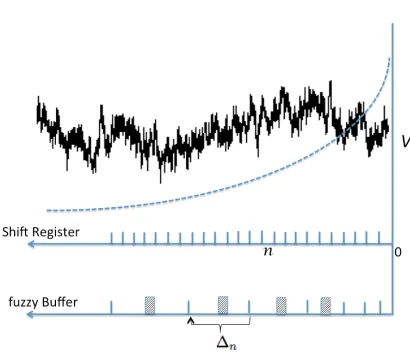
≃1/|n−m|α. Whenα≤1, the series will be long range correlated (Beran, 1994). The goal of the learner is to successfully predict the current valuevoatn=0. Figure 1 shows a sample time series leading up to the present moment. They-axis corresponds to the present moment and to its right lies the unknown future values of the time series. Thex-axis labeled as shift register denotes a memory buffer wherein eachvnis accurately stored in
Figure 1: A sample time seriesV with power-law two-point correlation is plotted w.r.t. time(n) with the current time step taken to ben=0. The figure contrasts the way in which the information is represented in a shift register and the fuzzy buffer. Each node of the fuzzy buffer linearly combines information from a bin containing multiple shift register nodes. The dashed curve shows the predictive information content from each time step that is relevant for predicting the future value of the time series.
a unique node. As we step forward in time, the information stored in each node will be transferred to its left-neighbor and the current valuevowill enter the first node. The shift register can thus self sufficiently evolve in real time. The longest time scale that can be represented with the shift register is linearly related to the number of nodes.
Given a limited number of memory nodes, what is the optimal way to representV in the memory so that the information relevant to prediction ofvois maximally preserved? We will show that this is achieved in the fuzzy buffer shown in Figure 1. Each node of the fuzzy buffer holds the average ofvns over a bin. For the fuzzy buffer, the widths of the bins increase linearly with the center of the bin; the bins are chosen to tile the past time line. Clearly, the accuracy of representingV is sacrificed in the process of compressing the information in an entire bin into a real number, but note that we attain the capacity to represent information from exponentially long timescales. With some analysis, we will show that sacrificing the accuracy with bin widths chosen in this way leads to maximal preservation of prediction-relevant information.
2.1 Deriving the Optimal Binning Strategy
To quantify the prediction relevant information contained in V, let us first review some general properties of the long range correlated series. Since our aim here is only to representV in memory and not to actually understand the generating mechanism underlyingV, it is sufficient to consider
V as being generated by a generic statistical algorithm, the ARFIMA model (Granger and Joyeux, 1980; Hosking, 1981; Wagenmakers et al., 2004). The basic idea behind the ARFIMA algorithm is that white noise at each time step can be fractionally integrated to generate a time series with long range correlations.2 Hence the time series can be viewed as being generated by an infinite auto-regressive generating function. In other words,vocan be generated from the past seriesV and an instantaneous Gaussian white noise inputηo.
vo=ηo+
∞
∑
n=1
a(n)vn. (1)
The ARFIMA algorithm specifies the coefficientsa(n)in terms of the exponentαin the two point correlation function.
a(n) = (−1)
n+1Γ(d+1)
Γ(n+1)Γ(d−n+1), (2)
whered is the fractional integration power given byd= (1−α)/2. The time series is stationary and long range correlated with finite variance only when d∈(0,1/2)orα∈(0,1) (Granger and Joyeux, 1980; Hosking, 1981). The asymptotic behavior of a(n) for large n can be obtained by applying Euler’s reflection formula and Stirling’s formula to approximate the Gamma functions in Equation 2. It turns out that when eitherdis small ornis large,
a(n)≃
Γ(d+1)sin(πd)
π
n−(1+d). (3)
For the sake of analytic tractability, the following analysis will focus only on small values ofd. From Equation 1, note thata(n)is a measure of the relevance ofvnin predictingvo, which we shall call the
P I C
-Predictive Information Content ofvn. Taylor expansion of Equation 3 shows that eacha(n)is linear indup to the leading order. Hence in smalldlimit, anyvnis a stochastic termηnplus a history dependent term of order
O
(d). Restricting to linear order ind, the totalP I C
ofvnandvm is simply the sum of their individualP I C
s, namelya(n) +a(m). Thus in the smalldlimit,P I C
is a simple measure of predictive information that is also an extensive quantity.When the entireV is accurately represented in an infinite shift register, the total
P I C
contained in the shift register is the sum of alla(n). This is clearly the maximum attainable value ofP I C
in any memory buffer, and it turns out to be 1.P I C
max=∞
∑
n=1
a(n) =1.
In a shift register withNmaxnodes, the total
P I C
isP I C
SRtot = Nmax∑
n=1
a(n) = 1−
∞
∑
Nmax
a(n) ≃ 1−sin(πd)Γ(d+1)
πd N
−d max,
d→0
−−→ dlnNmax. (4)
For any fixedNmax, whend is sufficiently small
P I C
SRtot will be very small. For example, whenNmax=100 andd=0.1,
P I C
SRtot ≃0.4. For smaller values ofd, observed in many natural signals,P I C
SRtot would be even lower. Whend=0.01, forNmaxas large as 10000, theP I C
SRtot is only 0.08. A large portion of the predictive information lies in long timescales. So the shift register is ill-suited to represent information from a long range correlated series.The
P I C
totfor a memory buffer can be increased if each of its nodes stored a linear combination of manyvns rather than a singlevnas in the shift register. This can be substantiated through informa-tion theoretic considerainforma-tions formulated by the Informainforma-tion Bottleneck (I B
) method (Tishby et al., 1999). A multi-dimensional Gaussian variable can be systematically compressed to lower dimen-sions by linear transformations while maximizing the relevant information content (Chechik et al., 2005). AlthoughV is a unidimensional time series in our consideration, at any moment the entireV can be considered as an infinite dimensional Gaussian variable since only its two point correla-tions are irreducible. Hence it heuristically follows from
I B
that linearly combining the variousvns into a given number of combinations and representing each of them in separate memory nodes should maximize the
P I C
tot. By examining Equation 1, it is immediately obvious that if we knew the values of a(n), the entireV could be linearly compressed into a single real number∑a(n)vn conveying all of the prediction relevant information. However, such a single-node memory buffer is not self sufficient: at each moment we explicitly need the entireV to update the value in that node. As an unbiased choice that does not requirea prioriknowledge of the statistics of the time series, we simply consider uniform averaging over a bin. Uniform averaging over a bin discards separate information about the time of the values contributing to the bin. Given this consideration, how should we space the bins to maximize theP I C
tot?Consider a bin ranging between n andn+∆n. We shall examine the effect of averaging all thevms within this bin and representing it in a single memory node. If all the vms in the bin are individually represented, then the
P I C
of the bin is∑ma(m). Compressing all thevms into their average would however lead to an error in prediction of vo; from Equation 1 this error is directly related to the extent to which thea(m)s within the bin are different from each other. Hence there should be a reduction in theP I C
of the bin. Given the monotonic functional form of a(n), the maximum reduction can only be∑m|a(m)−a(n)|. The netP I C
of the memory node representing the bin average is thenP I C
=n+∆n
∑
m=n
a(m) − n+∆n
∑
m=n|
a(n)−a(m)|,
≃ n ad(n)
"
2−2
1+∆n
n −d
−dn∆n
#
.
The series summation in the above equation is performed by approximating it as an integral in the large nlimit. The bin size that maximizes the
P I C
can be computed by setting the derivative ofP I C
w.r.t.∆nequal to zero. The optimal bin size and the correspondingP I C
turns out to be∆opt
n =
h
21/(1+d)−1in,
P I C
opt≃n a(n) dh
the nodes of the fuzzy buffer byN, ranging from 1 toNmax, and denote the starting point of each bin bynN, then
nN+1= (1+c)nN =⇒ nN =n1(1+c)(N−1), (6) where 1+c=21/(1+d). Note that the fuzzy buffer can represent information from timescales of the ordernNmax, which is exponentially large compared to the timescales represented by a shift register
withNmaxnodes. The total
P I C
of the fuzzy buffer,P I C
FBtot, can now be calculated by summing over theP I C
s of each of the bins. Focusing on small values ofd so thata(n)has the power law form for alln, applying Equations 3 and 5 yieldsP I C
FBtot ≃Nmax
∑
N=1
sin(πd)Γ(d+1)
πd
h
2+d−(1+d)21/(1+d)in−Nd.
Takingn1=1 andnN given by Equation 6,
P I C
FBtot ≃ sin(πd)Γ(d+1)πd
h
2+d−(1+d)21/(1+d)i
1−(1+c)−d Nmax
1−(1+c)−d
,
d→0
−−→ [ln 4−1]d Nmax. (7)
Comparing Equations 4 and 7, note that whendis small, the
P I C
FBtot of the fuzzy buffer grows linearly with Nmax while theP I C
SRtot of the shift register grows logarithmically with Nmax. For example, withNmax=100 andd=0.01, theP I C
FBtot of the fuzzy buffer is 0.28, while theP I C
SRtot of the shift register is only 0.045. Hence whenNmaxis relatively small, the fuzzy buffer represents a lot more predictive information than a shift register.The above description of the fuzzy buffer corresponds to the ideal case wherein the neighboring bins do not overlap and uniform averaging is performed within each bin. Its critical property of linearly increasing bin sizes ensures that the temporal accuracy of information is sacrificed optimally and in a scale-free fashion. However, this ideal fuzzy buffer cannot self sufficiently evolve in real time because at every moment allvns are explicitly needed for its construction. In the next section, we present a self sufficient memory system that possesses the critical property of the ideal fuzzy buffer, but differs from it by having overlapping bins and non-uniform weighted averaging within the bins. To the extent the self sufficient fuzzy memory system resembles the ideal fuzzy buffer, we can expect it to be useful in representing long range correlated signals in a resource-limited environment.
3. Constructing Self Sufficient Fuzzy Memory
In this section, we first describe a mathematical basis for representing the recent past in a scale-free fashion based on a neuro-cognitive model of internal time, TILT (Shankar and Howard, 2012). We then describe several critical considerations necessary to implement this representation of recent past into a discrete set of memory nodes. Like the ideal fuzzy buffer described in the Section 2, this memory representation will sacrifice temporal accuracy to represent prediction-relevant information over exponential time scales. But unlike the ideal fuzzy buffer, the resulting memory representation will be self sufficient, without requiring additional resources to construct the representation.
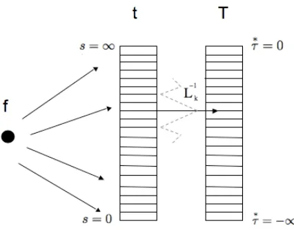
Figure 2: The scale-free fuzzy representation - Each node in thetcolumn is a leaky integrator with a specific decay constantsthat is driven by the functional valuef at each moment. The activity of thetcolumn is transcribed at each moment by the operatorL-1
k to represent the past functional values in a scale-free fuzzy fashion in theTcolumn.
accuracy that falls off in a scale-free fashion. This is achieved using two columns of nodest andT as shown in Figure 2. TheTcolumn estimatesf(τ)up to the present moment, while thet column is an intermediate step used to constructT. The nodes in thet column are leaky integrators with decay constants denoted bys. Each leaky integrator independently gets activated by the value off at any instant and gradually decays according to
dt(τ,s)
dτ =−st(τ,s) +f(τ). (8)
At every instant, the information in the t column is transcribed into the T column through a linear operatorL-1k.
T(τ,∗τ) = (−1) k
k! s
k+1t(k)(τ,s) : wheres=−k/τ∗. (9)
T ≡ L-1kt.
Herekis a positive integer andt(k)(τ,s)is thek-th derivative oft(τ,s)with respect tos. The nodes of theTcolumn are labeled by the parameterτ∗and are in one to one correspondence with the nodes of thetcolumn labeled bys. The correspondence betweensandτ∗is given bys=−k/∗τ. We refer toτ∗asinternal time; at any momentτ, aτ∗node estimates the value off at a timeτ+τ∗in the past. The range of values of s andτ∗ can be made as large as needed at the cost of resources, but for mathematical idealization we let them have an infinite range.
past time
internal time
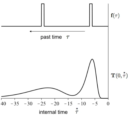
Figure 3: Taking the present moment to beτ=0, a samplef(τ)is plotted in the top, and the mo-mentary activity distributed across theTcolumn nodes is plotted in the bottom.
reconstruction of the history offfrom−∞toτ, that isT(τ,τ∗)≃f(τ+τ∗)for all values of∗τfrom 0 to −∞. Whenkis finiteT(τ,τ∗)is an inaccurate reconstruction of the history off. For example, taking the current moment to beτ=0, Figure 3 illustrates anf that is briefly non-zero aroundτ=−7 and
τ=−23. The reconstructed history off in theT column shows two peaks approximately around ∗
τ=−7 and τ∗=−23 . The value off at any particular moment in the past is thus smeared over a range of∗τvalues, and this range of smearing increases as we go deeper into the past. Thus, the more distant past is reconstructed with a lesser temporal accuracy.
Furthermore, it turns out that the smear is precisely scale invariant. To illustrate this, consider f(τ)to be a Dirac delta function at a moment τo in the past,f(τ) =δ(τ−τo), and let the present moment beτ=0. Applying Equations 8 and 9, we obtain
T(0,τ∗) = 1 |τo|
kk+1 k!
τo
∗
τ k+1
e−k(τo/
∗
τ). (10)
In the above equation bothτo and∗τare negative. T(0,∗τ) is the fuzzy reconstruction of the delta function input. T(0,τ∗) is a smooth peaked function whose height is proportional to 1/|τo|, width is proportional to|τo|, and the area is equal to 1. Its dependence on the ratio(τo/
∗
τ)ensures scale invariance—for anyτowe can linearly scale the
∗
above equation, which fork>2 turns out to be
σ[T(0,τ∗)] =√|τo|
k−2
k k−1
. (11)
Note thatkis the only free parameter that affects the smear;kindexes the smear in the representa-tion. The larger thek the smaller the smear. In the limitk→∞, the smear vanishes and the delta function input propagates into the T column exactly as delta function without spreading, as ifT were a shift register.
Though we tookf to be a simple delta function input to illustrate the scale invariance of theT representation, we can easily evaluate theTrepresentation of an arbitraryffrom Equations 8 and 9.
T(0,∗τ) =
Z 0
−∞
"
1
|τ∗| kk+1
k!
τ′
∗
τ k
e−k(τ′/
∗
τ)
#
f(τ′)dτ′. (12)
The fvalues from a range of past times are linearly combined and represented in eachτ∗node. The term in the square brackets in the above equation is the weighting function of the linear com-bination. Note that it is not a constant function over a circumscribed past time bin, rather it is a smooth function peaked at τ′ =∗τ, with a spread proportional to|τ∗|. Except for the fact that this weighting function is not uniform, the activity of a∗τnode has the desired property mimicking a bin of the ideal fuzzy buffer described in Section 2.
3.1 Self Sufficient Discretized Implementation
Although it appears from Equation 12 that theTrepresentation requires explicit information about thefvalues over the past time, recall that it can be constructed from instantaneoustrepresentation. Since Equation 8 is a local differential equation, the activity of each t node will independently evolve in real time, depending only on the present value of the node and the input available at that moment. Hence any discrete set oft nodes also evolves self sufficiently in real time. To the extent the activity in a discrete set ofTnodes can be constructed from a discrete set oftnodes, this memory system as a whole can self sufficiently evolve in real time. Since the activity of eachτ∗node in theT column is constructed independently of the activity of otherτ∗nodes, we can choose any discrete set ofτ∗values to form our memory system. In accordance with our analysis of the ideal fuzzy buffer in Section 2, we shall pick the following nodes.
∗
τmin,
∗
τmin(1+c),
∗
τmin(1+c)2, . . . ∗
τmin(1+c)(Nmax−1)=
∗
τmax. (13)
Together, these nodes form the fuzzy memory representation with Nmax nodes. The spacing in Equation 13 will yield several important properties.
Unlike the ideal fuzzy buffer described in Section 2, it is not possible to associate a circum-scribed bin for a node because the weighting function (see Equation 12) does not have compact support. Since the weighting function associated with neighboring nodes overlap with each other, it is convenient to view the bins associated with neighboring nodes as partially overlapping. The over-lap between neighboring bins implies that some information is redundantly represented in multiple nodes. We shall show in the forthcoming subsections that by appropriately tuning the parametersk
3.1.1 DISCRETIZEDDERIVATIVE
Although any set ofτ∗nodes could be picked to form the memory buffer, their activity is ultimately constructed from the nodes in thet column whosesvalues are given by the one to one correspon-dences=−k/τ∗. Since theLk-1operator has to take thek-th derivative along thesaxis,L-1k depends on the way thes-axis is discretized.
For any discrete set of svalues, we can define a linear operator that implements a discretized derivative. For notational convenience, let us denote the activity at any momentt(τ,s) as simply t(s). Sincetis a column vector with the rows labeled bys, we can construct a derivative matrix[D] such that
t(1)= [D]t =⇒ t(k)= [D]kt.
The individual elements in the square matrix[D]depends on the set ofsvalues. To compute these el-ements, consider any three successive nodes withsvaluess−1,so,s1. The discretized first derivative oftatsois given by
t(1)(so) =
t(s1)−t(so)
s1−so
so−s−1
s1−s−1
+t(so)−t(s−1)
so−s−1
s1−so
s1−s−1
.
The row in[D]corresponding to so will have non-zero entries only in the columns corresponding to s−1, so and s1. These three entries can be read out as coefficients of t(s−1), t(so) and t(s1) respectively in the r.h.s of the above equation. Thus the entire matrix[D]can be constructed from any chosen set ofsvalues. By taking thek-th power of[D], theL-1k operator can be straightforwardly constructed and the activity of the chosen set ofτ∗nodes can be calculated at each moment.3 This memory system can thus self sufficiently evolve in real time.
When the spacing between the nodes (controlled by the parameter c) is small, the discretized
k-th derivative will be accurate. Under uniform discretization of thesaxis, it can be shown that the relative error in computation of thek-th derivative due to discretization is of the order
O
(kδ2s/24), where δs is the distance between neighborings values (see appendix B of Shankar and Howard, 2012). Based on the s values corresponding to Equation 13, it turns out that the relative error in
the construction of the activity of a ∗τnode is
O
(k3c2/96∗τ2). For large ∗τ the error is quite small but for small∗τthe error can be significant. To curtail the discretization error, we need to holdτ∗min sufficiently far from zero. The error can also be controlled by choosing small c for large k and vice versa. If for practical purposes we require a very small ∗τmin, then ad hoc strategies can be adopted to control the error at low∗τnodes. For example, by relaxing the requirement of one to one correspondence between thet andTnodes, we can choose a separate set of closely spacedsvalues to exclusively compute the activity of each of the smallτ∗nodes.Finally, it has to be noted that the discretization error induced in this process should not be con-sidered as an error in the conventional sense of numerical solutions to differential equations. While numerically evolving differential equations with time-varying boundary conditions, the discretiza-tion error in the derivatives will propagate leading to large errors as we move farther away from the boundary at late times. But in the situation at hand, since the activity of eachτ∗node is computed independently of others, the discretization error does not propagate. Moreover, it should be noted
that the effect of discretization can be better viewed as coarse-graining thek-th derivative rather than as inducing an error in computing thek-th derivative. The fact that eachτ∗node ultimately holds a scale-free coarse-grained value of the input function (see Equation 12), suggests that we wouldn’t need the exactk-th derivative to construct its activity. To the extent the discretization is scale-free as in Equation 13, the T representation constructed from the coarse-grained k-th derivative will represent some scale free coarse grained value of the input; however the weighting function would not exactly match that in Equation 12. In other words, even if the discretized implementation does not accurately match the continuum limit, it still accurately satisfies the basic properties we require from a fuzzy memory system.
3.1.2 SIGNAL-TO-NOISERATIO WITHOPTIMALLY-SPACEDNODES
The linearity of Equations 8 and 9 implies that any noise in the input functionf(τ)will exactly be represented inT without any amplification. However when there is random uncorrelated noise in thetnodes, the discretizedL-1k operator can amplify that noise, more so ifcis very small. It turns out that choice of nodes according to Equation 13 results in a constant signal-to-noise ratio across time scales.
If uncorrelated noise with standard deviationηis added to the activation of each of thetnodes, then theL-1k operator combines the noise from 2kneighboring nodes leading to a noisyT represen-tation. If the spacing between the nodes neighboring asnode isδs, then the standard deviation of the noise generated by theL-1
k operator is approximatelyη √
2ksk+1/δk
sk!. To view this noise in an appropriate context, we can compare it to the magnitude of the representation of a delta function signal at a past timeτo=−k/s(see Equation 10). The magnitude of theTrepresentation for a delta function signal is approximately kke−ks/k!. The signal to noise ratio (SNR) for a delta function signal is then
SNR=η−1
k[δs/s] √
2e k
. (14)
If the spacing between neighboring nodes changes such that[δs/s]remains a constant for alls, then the signal to noise ratio will remain constant over all timescales. This would however require that the nodes are picked according to Equation 13, making SNR =η−1(kc/√2e)k. Any other set of nodes would make the signal to noise ratio zero either at large or small timescales.
This calculation however does not represent the most realistic situation. Because thetnodes are leaky integrators (Equation 8), the white noise present across time will accumulate and hence nodes with long time constants should have a higher value ofη. In fact, the standard deviation of white noise in thet nodes should go down withsaccording toη ∝1/√s. From Equation 14, we can then
conclude that the SNR of large ∗τnodes should drop down to zero as 1/ q
|τ∗|. However, because each∗τnode represents a weighted temporal average of the past signal, it is not appropriate to use an isolated delta function signal to estimate the signal to noise ratio. It is more appropriate to compare temporally averaged noise to a temporally spread signal. We consider two such signals. (i) Suppose f(τ)itself is a temporally uncorrelated white noise like signal. The standard deviation in the activity
of aτ∗node in response to this signal is proportional to 1/ q
The total expected number of spikes that would be generated in the timescale of integration of a∗τ
node is simply
q
|τ∗|. Consequently, the expectation value of the activity of a∗τnode in response to
this signal would be
q
|∗τ|multiplied by the magnitude of representation of a single delta function. The SNR for this signal is again a constant over allτ∗nodes. So, we conclude that for any realistic stationary signal spread out in time, the SNR will be a constant over all timescales as long as the nodes are chosen according to Equation 13.
3.2 Information Redundancy
The fact that a delta function input inf is smeared over manyτ∗ nodes implies that there is a re-dundancy in information representation in theT column. In a truly scale-free memory buffer, the redundancy in information representation should be equally spread over all time scales represented in the buffer. The information redundancy can be quantified in terms of the mutual information shared between neighboring nodes in the buffer. In the appendix, it is shown that in the presence of scale free input signals, the mutual information shared by any two neighboring buffer nodes can be a constant only if theτ∗nodes are distributed according to Equation 13. Consequently information redundancy is uniformly spread only when theτ∗nodes are given by Equation 13.
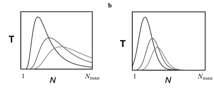
The uniform spread of information redundancy can be intuitively understood by analyzing how a delta function input spreads through the buffer nodes as time progresses. Figure 4 shows the activity of the buffer nodes at three points in time following the input. In Figure 4a where the ∗
τ values of the buffer nodes are chosen to be equidistant, the activity is smeared over more and more number of nodes as time progresses. This implies that the information redundancy is large in the nodes representing long timescales. In Figure 4b where the τ∗ values of the buffer nodes are chosen according to Equation 13, the activity pattern does not smear, instead the activity as a whole gets translated with an overall reduction in size. The translational invariance of the activity pattern as it passes through the buffer nodes explains why the information redundancy between any two neighboring nodes is a constant. The translational invariance of the activity pattern can be analytically established as follows.
Consider two different values of τo in Equation 10, sayτ1 andτ2. Let the corresponding T activities be T1(0,τ∗) and T2(0,∗τ) respectively. If the τ∗ value of the N-th node in the buffer is given byτ∗N, then the pattern of activity across the nodes is translationally invariant if and only if T1(0,
∗
τN)∝T2(0,
∗
τN+m)for some constant integerm. For this to hold true, we need the quantity
T1(0,τ∗N)
T2(0,τ∗N+m) =
τ1
τ2
k"∗
τN+m
∗
τN
#k+1 ek
τ1
∗
τN− τ2
∗τ
N+m
to be independent ofN. This is possible only when the quantity inside the power law form and the exponential form are separately independent ofN. The power law form can be independent of
N only ifτ∗N∝(1+c)N, which implies the buffer nodes have ∗
τvalues given by Equation 13. The exponential form is generally dependent on N except when its argument is zero, which happens whenever(1+c)m=τ
a b
Figure 4: Activity of the fuzzy memory nodes in response to a delta function input at three dif-ferent times with (a) uniformly spaced nodes and (b) nodes chosen in accordance with Equation 13.
anyτ2. Hence, the translational invariance of the activity pattern holds only when the∗τvalues of the buffer nodes conform to Equation 13.
3.3 Balancing Information Redundancy and Information Loss
We have seen that the choice ofτ∗nodes in accordance with Equation 13 ensures that the information redundancy is equally distributed over the buffer nodes. However, equal distribution of information redundancy is not sufficient; we would also like to minimize information redundancy. It turns out that we cannot arbitrarily reduce the information redundancy without creating information loss. The parametersk andchave to be tuned in order to balance information redundancy and information loss. Ifkis too small for a givenc, then many nodes in the buffer will respond to input from any given moment in the past, resulting in information redundancy. On the other hand, ifkis too large for a givenc, the information from many moments in the past will be left unrepresented in any of the buffer nodes, resulting in information loss. So we need to match c withk to simultaneously minimize both information redundancy and information loss.
This can be achieved if the information from any given moment in the past is not distributed over more than two neighboring buffer nodes. To formalize this, consider a delta function input at a timeτoin the past and let the current moment beτ=0. Let us look at the activity induced by this input (Equation 10) in four successive buffer nodes,N−1,N andN+1 andN+2. Theτ∗ values of these nodes are given by Equation 13, for instance∗τN=
∗
τmin(1+c)N−1and
∗
τN+1=∗τmin(1+c)N.
From Equation 10, it can be seen that theN-th node attains its maximum activity when τo=τ∗N and the(N+1)-th node attains its maximum activity whenτo=
∗
τN+1, and for all the intervening times ofτobetween
∗
τNand
∗
a b
!"
#"
Activity due to stimulus at
k = 2
k = 12
k = 100
k = 12
0 0.5 1.0
(input time)
T
otal activity of nodes N and N+1
k = 8 k = 4
k = 30
k = 100
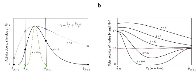
Figure 5: a. The activity of four successive fuzzy memory nodes N−1, N,N+1, andN+2 in response to a delta function input at a past moment τo that falls right in between the timescales of theN-th and the(N+1)-th nodes. The nodes are chosen according to the distribution given by Equation 13 withc=1. b. The sum of activity of the N-th and (N+1)-th nodes in response to a delta function input at various timesτoranging between the timescales ofN-th and(N+1)-th nodes. For eachk, the activities are normalized to have values in the range of 0 to 1.
Figure 5a plots the activity of the four successive nodes with c=1, whenτo is exactly in the middle ofτ∗N and
∗
τN+1. For each value ofk, the activity is normalized so that it lies between 0 and 1. The four vertical lines represent the 4 nodes and the dots represent the activity of the corresponding nodes. Note that fork=2 the activity of all 4 nodes is substantially different from zero, implying a significant information redundancy. At the other extreme,k=100, the activity of all the nodes are almost zero, implying that the information about the delta function input at timeτo= (τ∗N+τ∗N+1)/2 has been lost. To minimize both the information loss and the information redundancy, the value of
kshould be neither too large nor too small. Note that fork=12, the activities of the(N−1)-th and the(N+2)-th nodes are almost zero, but activities of theN-th and(N+1)-th nodes are non-zero.
For any givenc, a rough estimate of the appropriatekcan be obtained by matching the difference in theτ∗values of the neighboring nodes to the smearσfrom Equation 11.
σ= |
∗
τN+1|
√
k−2
k k−1
≃ |τ∗N+1−τ∗N| ⇒
k
(k−1)√k−2 ≃
c
1+c. (15)
This condition implies that a large value ofkwill be required whencis small and a small value of
kwill be required whencis large. In particular, Equation 15 suggests thatk≃8 whenc=1, which will be the parameters we pick for the demonstrations in Section 4.
To further illustrate the information loss at high values ofk, Figure 5b shows the sum of activity of the N-th and the (N+1)-th nodes for all values of τo between
∗
τN and
∗
τN+1. For each k, the activities are normalized so that theN-th node attains 1 when τo=
∗
τN. Focusing on the case of
k=100 in Figure 5b, there is a range of τo values for which the total activity of the two nodes is very close to zero. The input is represented by the N-th node when τo is close to
∗
total activity of the two nodes not have a local minimum—in other words the minimum should be at the boundary, atτo=
∗
τN+1. This is apparent in Figure 5b fork=4, 8 and 12. Forc=1, it turns out that there exists a local minimum in the summed activity of the two nodes only for values of
k greater than 12. For any given c, the appropriate value of k that simultaneously minimizes the information redundancy and information loss is the maximum value ofkfor which a plot similar to Figure 5b will not have a local minimum.
In summary, the fuzzy memory system is the set of T column nodes withτ∗ values given by Equation 13, with the value ofkappropriately matched withcto minimize information redundancy and information loss.
4. Time Series Forecasting
We compare the performance of the self-sufficient fuzzy memory to a shift register in time series forecasting with a few simple illustrations. Our goal here is to illustrate the differences between a simple shift register and the self-sufficient fuzzy memory. Because our interest is in representation of the time series and not in the sophistication of the learning algorithm, we use simple linear regression algorithm to learn and forecast these time series.
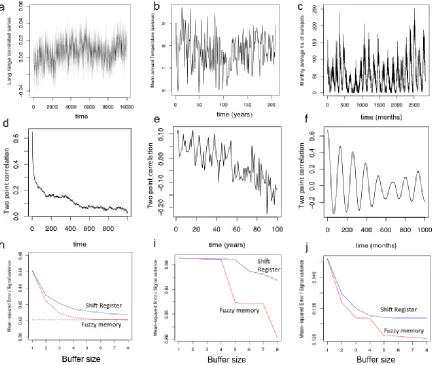
We consider three time series with different properties. The first was generated by fractionally integrating white noise (Wagenmakers et al., 2004) in a manner similar to that described in Section 2. The second and third time series were obtained from the online library at http://datamarket.com. The second time series is the mean annual temperature of the Earth from the year 1781 to 1988. The third time series is the monthly average number of sunspots from the year 1749 to 1983 measured from Zurich, Switzerland. These three time series are plotted in the top row of Figure 6. The corresponding two point correlation function of each series is plotted in the middle row of Fig-ure 6. Examination of the two point correlation functions reveal differences between the series. The fractionally-integrated noise series shows long-range correlations falling off like a power law. The temperature series shows correlations near zero (but modestly positive) over short ranges and weak negative correlation over longer times. The sunspots data has both strong positive short-range autocorrelation and a longer range negative correlation, balanced by a periodicity of 130 months corresponding to the 11 year solar cycle.
4.1 Learning and Forecasting Methodology
Let Nmax denote the total number of nodes in the memory representation and letN be an index corresponding to each node ranging from 1 to Nmax. We shall denote the value contained in the nodes at any time stepiby Bi[N]. The time series was sequentially fed into both the shift register and the self-sufficient fuzzy memory and the representations were evolved appropriately at each time step. The values in the shift register nodes were shifted downstream at each time step as discussed Section 2. At any instant the shift register held information from exactlyNmaxtime steps in the past. The values in the self-sufficient fuzzy memory were evolved as described in Section 3, withτ∗ values taken to be 1, 2, 4, 8, 16, 32,...2(Nmax−1), conforming to Equation 13 with ∗τ
min=1,
c=1 andk=8.
Figure 6: (a) Simulated time series with long range correlations based on ARFIMA model with
at each time stepPiand the squared error in predictionEiare
Pi=I+ Nmax
∑
N=1
RNBi[N], Ei= [Pi−Vi]2.
The regression coefficients were extracted by minimizing the total squared errorE=∑iEi. For this purpose, we used a standard procedurelm()in the open source software R.
The accuracy of forecast is inversely related to the total squared error E. To get an absolute measure of accuracy we have to factor out the intrinsic variability of the time series. In the bottom row of Figure 6, we plot the mean of the squared error divided by the intrinsic variance in the time series Var[Vi]. This quantity would range from 0 to 1; the closer it is to zero, the more accurate the prediction.
4.1.1 LONGRANGECORRELATEDSERIES
The long range correlated series (Figure 6a) is by definition constructed to yield a two point corre-lation that decays as a power law. This is evident from its two point correcorre-lation in Figure 6d that is decaying, but always positive. Since the value of the series at any time step is highly correlated with its value at the previous time step, we can expect to generate a reasonable forecast using a single node that holds the value from the previous time step. This can be seen from Figure 6h, where the error in forecast is only 0.46 with a single node. Adding more nodes reduces the error for both the shift register and the self-sufficient fuzzy memory. But for a given number of nodes, the fuzzy memory always has a lower error than the shift register. This can be seen from Figure 6h where the curve corresponding to the fuzzy memory falls below that of the shift register.
Since this series is generated by fractionally integrating white noise, the mean squared error cannot in principle be lower than the variance of the white noise used for construction. That is, there is a lower bound for the error that can be achieved in Figure 6h. The dotted line in Figure 6h indicates this bound. Note that the fuzzy memory approaches this bound with a smaller number of nodes than the shift register.
4.1.2 TEMPERATURESERIES
The temperature series (Figure 6b) is much more noisy than the long range correlated series, and seems structureless. This can be seen from the small values of its two point correlations in Figure 6e. This is also reflected in the fact that with a small number of nodes, the error is very high. Hence it can be concluded that no reliable short range correlation exist in this series. That is, knowing the average temperature during a given year does not help much in predicting the average temperature of the subsequent year. However, there seems to be a weak negative correlation at longer scales that could be exploited in forecasting. Note from Figure 6i that with additional nodes the fuzzy memory performs better at forecasting and has a lower error in forecasting than a shift register. This is because the fuzzy memory can represent much longer timescales than the shift register of equal size, and thereby exploit the long range correlations that exist.
4.1.3 SUNSPOTSSERIES
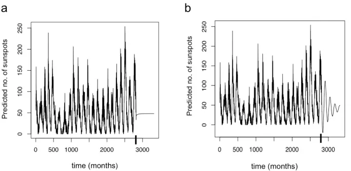
Figure 7: Forecasting the distant future. The sunspots time series of length 2820 is extrapolated for 500 time steps in the future using(a)shift register with 8 nodes, and(b)fuzzy memory with 8 nodes. The solid tick mark on thex-axis at 2820 corresponds to the point where the original series ends and the predicted future series begins.
even a single node that holds the value from the previous time step is sufficient to forecast with an error of 0.15, as seen in Figure 6j. As before, with more nodes, the fuzzy memory consistently has a lower error in forecasting than the shift register with equal number of nodes. Note that when the number of nodes is increased from 4 to 8, the shift register does not improve in accuracy while the fuzzy memory continues to improve in accuracy.
With a single node, both fuzzy memory and shift register essentially just store the information from the previous time step. Because most of the variance in the series can be captured by the information in the first node, the difference between the fuzzy memory and the shift register with additional nodes is not numerically overwhelming when viewed in Figure 6j. However, there is a qualitative difference in the properties of the signal extracted by the two memory systems. In order to successfully learn the 130 month periodicity, the information about high positive short range correlations is not sufficient, it is essential to also learn the information about the negative correlations at longer time scales. From Figure 6f, note that the negative correlations exist at a timescale of 50 to 100 months. Hence in order to learn this information, these timescales have to be represented. A shift register with 8 nodes cannot represent these timescales but the fuzzy memory with 8 nodes can.
a b
1 2 3 4 5 6 7 8
0.130
0.140
0.150
Buffersize
Mean−squared Error / Signal v
ar
iance
Fuzzy memory Shift Register
1 2 3 4 5 6 7 8
0.125
0.135
0.145
Buffersize
Mean−squared Error / Signal v
ar
iance
Fuzzy memory Shift Register Subsampled−5 Subsampled−10
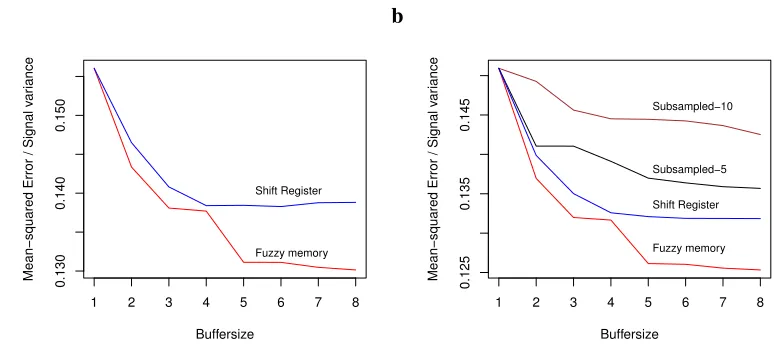
Figure 8: a. Testing error in forecasting. The regression coefficients were extracted from the first half of the sunspot series and testing was performed on the second half of the series. b. Forecasting error of the fuzzy memory, shift register and subsampled shift register with a node spacing of 5 and 10.
the original series ends and the predicted future series begins. Note that the series forecasted by the shift register immediately settles on the mean value without oscillation. This is because the time scale at which the oscillations are manifest is not represented by the shift register with 8 nodes. Figure 7b shows the series generated by the fuzzy memory with 8 nodes. Note that the series predicted by the fuzzy memory continues in an oscillating fashion with decreasing amplitude for several cycles eventually settling at the mean value. This is possible because the fuzzy memory represents the signal at a sufficiently long time scale to capture the negative correlations in the two-point correlation function.
Of course, a shift register with many more nodes can capture the long-range correlations and predict the periodic oscillations in the signal. However the number of nodes necessary to describe the oscillatory nature of the signal needs to be of the order of the periodicity of the oscillation, about 130 in this case. This would lead to overfitting the data. At least in the case of the simple linear regression algorithm, the number of regression coefficients to be extracted from the data increases with the number of nodes, and extracting a large number of regression coefficients from a finite data set will unquestionably lead to overfitting the data. Hence it would be ideal to use the least number of nodes required to span the relevant time scale.
In order to ensure that the extracted regression coefficients has not overfitted the data, we split the sunspots time series into two halves. We extracted the regression coefficients by using only the first half for training and used the second half for testing the predictions generated by those coefficients. Figure 8a plots this testing error, and should be compared to the training error plotted in Figure 6j. Other than the noticeable fact that the testing error is slightly higher than the training error, the shape of the two plots are very similar for both fuzzy memory and the shift register.
information from both positive and negative correlations can be obtained. Although the subsampled shift register contains relatively few nodes, it cannot self sufficiently evolve in real time; we would need the resources associated with the complete shift register in order to evolve the memory at each moment. By subsampling 8 equidistantly spaced nodes of the shift register 1,11,21,31,...81, and extracting the corresponding regression coefficients, it is possible to extend the series to have an oscillatory structure analogous to Figure 7b. However it turns out that the forecasting error for the subsampled shift register is significantly higher than the forecasting error from the fuzzy memory. Figure 8b shows the forecasting error for subsampled shift register with equidistant node spacing of 5 and 10. Even though the subsampled shift register with a node spacing of 10 extends over a similar temporal range as the fuzzy memory, and captures the oscillatory structure in the data, the fuzzy memory outperforms it with a lower error. The advantage of the fuzzy memory over the subsampled shift register comes from the property of averaging over many previous values at long time scales rather than picking a single noisy value and using that for prediction. This property helps to suppress unreliable fluctuations that could lead to overfitting the data.
5. Discussion
The fuzzy memory holds more predictively relevant information than a shift register with the same number of nodes for long-range correlated signals, and hence performs better in time series fore-casting such signals. However, learning the relevant statistics from a lengthy time series is not the same as learning from very few learning trials. To learn from very few learning trials, a learner must necessarily make some generalizations based on some built-in assumptions about the environment. Since the fuzzy memory discards information about the precise time of a stimulus presentation, the temporal inaccuracy in memory can help the learner make such a generalization. Suppose it is use-ful for a learner to learn the temporal relationship between two events, say A and B. Let the statistics of the world be such that B consistently follows A after a delay period, which on each learning trial is chosen from an unknown distribution. After many learning trials, a learner relying on a shift register memory would be able to sample the entire distribution of delays and learn it precisely. But real world learners may have to learn much faster. Because the fuzzy memory system represents the past information in a smeared fashion, a single training sample from the distribution will naturally let the learner make a scale-free temporal generalization about the distribution of delays between A and B. The temporal profile of this generalization will not in general match the true distribution that could be learned after many learning trials, however the fact that it is available after a single learning trial provides a tremendous advantage for natural learners.
5.1 Neural Networks with Temporal Memory
Let us now consider the fuzzy memory system in the context of neural networks with temporal memory. It has been realized that neural networks with generic recurrent connectivity can have sufficiently rich dynamics to hold temporal memory of the past. Analogous to how the ripple pat-terns on a liquid surface contains information about the past perturbations, the instantaneous state of the recurrent network holds the memory of the past which can be simply extracted by training a linear readout layer. Such networks can be implemented either with analog neurons-echo state networks (Jaeger, 2001), or with spiking neurons-liquid state machines (Maass et al., 2002). They are known to be non-chaotic and dynamically stable as long as their spectral radius or the largest eigenvalue of the connectivity matrix has a magnitude less than one. Abstractly, such networks with fixed recurrent connectivity can be viewed as a reservoir of nodes and can be efficiently used for computational tasks involving time varying inputs, including time series prediction (Wyffels and Schrauwen, 2010).
The timescale of these reservoirs can be tuned up by introducing leaky integrator neurons in them (Jaeger et al., 2007). However, a reservoir with finite nodes cannot have memory from infinite past. In fact the criterion for dynamical stability of the reservoir is equivalent to requiring a fading memory (Jaeger, 2002). If we define a memory function of the reservoir to be the precision with which inputs from each past moment can be reconstructed, it turns out that the net memory, or the area under the memory function over all past times, is bounded by the number of nodes in the reservoirNmax. The exact shape of the memory function will however depend on the connectivity within reservoir. For a simple shift register connectivity, the memory function is a step function which is 1 up to Nmax time steps in the past and zero beyond Nmax. But for a generic random connectivity the memory function decays smoothly, sometimes exponentially and sometimes as a power law depending on the spectral radius (Ganguli et al., 2008). For linear recurrent networks, it turns out that the memory function is analytically tractable at least in some special cases (White et al., 2004; Hermans and Schrauwen, 2010), while the presence of any nonlinearity seems to reduce the net memory (Ganguli et al., 2008). By increasing the number of nodes in the reservoir, the net memory can be increased. But unless the network is well tailored, as in orthogonal networks (White et al., 2004) or a divergent feed-forward networks (Ganguli et al., 2008), the net memory grows very slowly and sub-linearly with the number of nodes. Moreover, analysis of trajectories in the state-space of a randomly connected network suggests that the net memory will be very low when the connectivity is dense (Wallace et al., 2013).
5.2 Unaddressed Issues
Two basic issues essential to real-world machine learning applications have been ignored in this work for the sake of theoretical simplicity. First is that we have simply focused on a scalar time varying signal, while any serious learning problem would involve multidimensional signals. When unlimited storage resources are available, each dimension can be separately represented in a lengthy shift register. To conserve storage resources associated with the time dimension, we could replace the shift register with the self-sufficient fuzzy memory. This work however does not address the issue of conserving storage resources by compressing the intrinsic dimensionality of the signal. In general, most of the information relevant for future prediction is encoded in few combinations of the various dimensions of the signal, called features. Techniques based on information bottleneck method (Creutzig and Sprekeler, 2008; Creutzig et al., 2009) and slow feature analysis (Wiskott and Sejnowski, 2002) can efficiently extract these features. The strategy of representing the time series in a scale invariantly fuzzy fashion could be seen as complementary to these techniques. For instance, slow feature analysis (Wiskott and Sejnowski, 2002) imposes the slowness principle where low-dimensional features that change most slowly are of interest. If the components of a time varying high dimensional signal is represented in a temporally fuzzy fashion rather than in a shift register, then we could potentially extract the slowly varying parts in an online fashion by examining differences in the activities of the largest two∗τnodes.
The second issue is that we have ignored the learning and prediction mechanisms while simply focusing on the memory representation. For simplicity we used the linear regression predictor in Section 4. Any serious application should involve the ability to learn nonlinearities. Support vector machines (SVM) adopt an elegant strategy of using nonlinear kernel functions to map the input data to a high dimensional space where linear methods can be used (Vapnik, 1998; M¨uller et al., 1997). The standard method for training SVMs on time series prediction requires feeding in the data from a sliding time window, in other words providing shift registers as input. It has recently been suggested that rather than using standard SVM kernels on sliding time window, if we used recurrent kernel functions corresponding to infinite recurrent networks, performance can be improved on certain tasks (Hermans and Schrauwen, 2012). This suggests that the gradually fading temporal memory of the recurrent kernel functions is more effective than the step-function memory of shift register used in standard SVMs for time series prediction. Training SVMs with standard kernel functions along with fuzzy memory inputs rather than shift register inputs is an alternative strategy for approaching problems involving signals with long range temporal correlations. Moreover, sincetnodes contain all the temporal information needed to construct the fuzzy memory, directly training the SVMs with inputs fromtnodes could also be very fruitful.
6. Conclusion
Signals with long-range temporal correlations are found throughout the natural world. Such signals present a distinct challenge to machine learners that rely on a shift-register representation of the time series. Here we have described a method for constructing a self-sufficient scale-free representation of temporal history. The nodes are chosen in a way that minimizes information redundancy and in-formation loss while equally distributing them over all time scales. Although the temporal accuracy of the signal is sacrificed, predictively relevant information from exponentially long timescales is available in the fuzzy memory system when compared to a shift register with the same number of nodes. This could be an extremely useful way to represent time series with long-range correlations for use in machine learning applications.
Acknowledgments
The authors acknowledge support from National Science Foundation grant, NSF BCS-1058937, and Air Force Office of Scientific Research grant AFOSR FA9550-12-1-0369.
Appendix A. Information Redundancy Across Nodes
The information redundancy in the memory representation can be quantified by deriving expressions for mutual information shared between neighboring nodes. When the input signal is uncorrelated or has scale-free long range correlations, it will be shown that the information redundancy is equally spread over all nodes only when theτ∗values of the nodes are given by Equation 13.
Takingf(τ)to be a stochastic signal and the current moment to beτ=0, the activity of aτ∗node in theTcolumn is (see Equation 12)
T(0,∗τ) =k k+1
k!
Z 0
−∞
1
|∗τ|
τ′
∗
τ k
e−k
τ′
∗
τ
f(τ′)dτ′.
The expectation value of this node can be calculated by simply averaging over f(τ′) inside the integral, which should be a constant if it is generated by a stationary process. By definingz=τ′/∗τ, we find that the expectation ofTis proportional to the expectation off.
T(0,τ∗)
=
fk k+1
k!
Z ∞
0
zke−kzdz.
A.1 White Noise Input
Letf(τ)to be white noise, that is
f
=0 and
f(τ)f(τ′)
∼δ(τ−τ′). The variance in the activity of each∗τnode is then given by
T2(0,∗τ)
=
kk+1
k!
2Z 0
−∞
Z 0
−∞
1
|∗τ|2
τ
∗
τ k
e−k
τ ∗τ τ′ ∗ τ k
e−k
τ′ ∗ τ
f(τ)f(τ′) dτdτ′,
= 1 |∗τ|
kk+1
k!
2Z ∞
0 z
2ke−2kzdz. (16)
As expected, the variance of a large|τ∗|node is small because the activity in this node is constructed by integrating the input function over a large timescale. This induces an artificial temporal correla-tion in that node’s activity which does not exist in the input funccorrela-tion. To see this more clearly, we calculate the correlation across time in the activity of one node, at timeτandτ′. With the definition
δ=|τ−τ′|/|∗τ|, it turns out that
T(τ,τ∗)T(τ′,∗τ)
=|τ∗|−1
kk+1 k!
2 e−kδ
k
∑
r=0
δk−r k!
r!(k−r)!
Z ∞
0
zk+re−2kzdz. (17) Note that this correlation is nonzero for anyδ>0, and it decays exponentially for largeδ. Hence even a temporally uncorrelated white noise input leads to short range temporal correlations in a∗τ
node. It is important to emphasize here that such temporal correlations will not be introduced in a shift register. This is because, in a shift register the functional value off at each moment is just passed on to the downstream nodes without being integrated, and the temporal autocorrelation in the activity of any node will simply reflect the temporal correlation in the input function.
Let us now consider the instantaneous correlation in the activity of two different nodes. At any instant, the activity of two different nodes in a shift register will be uncorrelated in response to a white noise input. The different nodes in a shift register carry completely different information, making their mutual information zero. But in theTcolumn, since the information is smeared across differentτ∗nodes, the mutual information shared by different nodes is non-zero. The instantaneous correlation between two different nodesτ∗1andτ∗2can be calculated to be
T(0,τ∗1)T(0,τ∗2)
= |τ∗2|−1
kk+1
k!
2Z ∞
0 z 2k(τ∗
1/τ∗2)ke−kz(1+
∗
τ1/∗τ2)dz,
∝ (
∗
τ1τ∗2)k
(|τ∗1|+| ∗
τ2|)2k+1
.
The instantaneous correlation in the activity of the two nodesτ∗1andτ∗2is a measure of the mutual information represented by them. Factoring out the individual variances of the two nodes, we have the following measure for the mutual information.
I
(τ∗1,τ∗2) =
T(0,∗τ1)T(0,∗τ2) q
T2(0,τ∗1)
T2(0,τ∗2) ∝
q
∗
τ1/τ∗2
(1+∗τ1/∗τ2)
2k+1
This quantity is high when ∗τ1/∗τ2 is close to 1. That is, the mutual information shared between neighboring nodes will be high when theirτ∗values are very close.
The fact that the mutual information shared by neighboring nodes is non-vanishing implies that there is redundancy in the representation of the information. If we require the information redun-dancy to be equally distributed over all the nodes, then we need the mutual information between any two neighboring nodes to be a constant. If∗τ1and
∗
τ2are any two neighboring nodes, then in order for
I
(∗τ1,∗τ2)to be a constant,τ∗1/τ∗2should be a constant. This can happen only if theτ∗values of the nodes are arranged in the form given by Equation 13.A.2 Long Range Correlated Input
Now consider f(τ) such that f(τ)f(τ′)
∼1/|τ−τ′|αfor large values of |τ−τ′|. Reworking the calculations analogous to those leading to Equation 17, we find that the temporal correlation is
T(τ,τ∗)T(τ′,∗τ)
= | ∗
τ|−α
2.4k
kk+1 k! 2 k
∑
r=0 Cr Z ∞ −∞|v|k−r
|v+δ|αe−
k|v|dv.
Hereδ=|τ−τ′|/|τ∗|andCr= k!k+r)! r!(k−r)!
2k−r
(k)k+r+1. The exact value ofCr is unimportant and we only
need to note that it is a positive number.
For α>1, the above integral diverges atv=−δ, however we are only interested in the case
α<1. Whenδis very large, the entire contribution to the integral comes from the region|v| ≪δ
and the denominator of the integrand can be approximated asδα. In effect,
T(τ,∗τ)T(τ′,∗τ)
∼ |∗τ|−αδ−α=|τ−τ′|−α
for large|τ−τ′|. The temporal autocorrelation of the activity of any node should exactly reflect the temporal correlations in the input when|τ−τ′|is much larger than the time scale of integration of that node (∗τ). As a point of comparison, it is useful to note that any node in a shift register will also exactly reflect the correlations in the input.
Now consider the instantaneous correlations across different nodes. The instantaneous correla-tion between two nodesτ∗1and∗τ2turns out to be
T(0,τ∗1)T(0, ∗
τ2)
=|τ∗2|−α
kk+1 k! 2 k
∑
r=0 Xrβk−r(1+βr−α+1)
(1+β)2k−r+1 . (18) Hereβ=|∗τ1|/|∗τ2|and eachXris a positive coefficient. By always choosing|τ∗2| ≥ |τ∗1|, we note two limiting cases of interest,β≪1 andβ≃1. Whenβ≪1, ther=kterm in the summation of the above equation yields the leading term, and the correlation is simply proportional to|τ∗2|−α, which is approximately equal to|∗τ2−τ∗1|−α. In this limit where|∗τ2| ≫ |τ∗1|, the correlation between the two nodes behaves like the correlation between two shift register nodes. When β≃1, note from Equation 18 that the correlation will still be proportional to|τ∗2|−α. Now if
∗
τ1and
∗
τ2are neighboring nodes with close enough values, we can evaluate the mutual information between them to be
I
(τ∗1,∗τ2) =
T(0,∗τ1)T(0,∗τ2) q
T2(0,τ∗1)
T2(0,τ∗2)
Reiterating our requirement from before that the mutual information shared by neighboring nodes at all scales should be the same, we are once again led to chooseτ∗2/
∗
τ1to be a constant which is possible only when the∗τvalues of the nodes are given by Equation 13.
References
R. T. Baillie. Long memory processes and fractional integration in econometrics.Journal of Econo-metrics, 73:5–59, 1996.
P. D. Balsam and C. R. Gallistel. Temporal maps and informativeness in associative learning.Trends in Neuroscience, 32(2):73–78, 2009.
J. Beran. Statistics for Long-Memory Processes. Chapman & Hall, New York, 1994.
G. Chechik, A. Globerson, N. Tishby, and Y. Weiss. Information bottleneck for gaussian variables.
Journal of Machine Learning Research, 6:165–188, 2005.
F. Creutzig and H. Sprekeler. Predictive coding and the slowness principle: An information-theoretic approach. Neural Computation, 20(4):1026–1041, 2008.
F. Creutzig, A. Globerson, and N. Tishby. Past-future information bottleneck in dynamical systems.
Physical Review E, 79:041925, 2009.
C. Donkin and R. M. Nosofsky. A power-law model of psychological memory strength in short-and long-term recognition. Psychological Science, 23:625–634, 2012.
D. J. Field. Relations between the statistics of natural images and the response properties of cortical cells. Journal of Optical Society of America A, 4:2379–2394, 1987.
C. R. Gallistel and J. Gibbon. Time, rate, and conditioning.Psychological Review, 107(2):289–344, 2000.
S. Ganguli, D. Huh, and H. Sompolinsky. Memory traces in dynamical systems. Proceedings of the National Academy of Sciences of the United States of America, 105(48):18970–18975, 2008.
D. L. Gilden. Cognitive emissions of 1/f noise.Psychological Review, 108:33–56, 2001.
C. W. J. Granger and R. Joyeux. An introduction to long-memory time series models and fractional differencing. Journal of Time Series Analysis, 1:15–29, 1980.
M. Hermans and B. Schrauwen. Memory in linear recurrent neural networks in continuous time.
Neural Networks, 23(3):341–355, 2010.
M. Hermans and B. Schrauwen. Recurrent kernel machines: Computing with infinite echo state networks. Neural Computation, 24(1):104–133, 2012.
G. E. Hinton, S. Osindero, and Y. W. Teh. A fast learning algorithm for deep belief nets. Neural Computation, 18:1527–1554, 2006.
H. Jaeger. The echo state approach to analyzing and training recurrent networks. GMD-Report 148, GMD - German National Research Institute for Information Technology, 2001.
H. Jaeger. Short term memory in echo state networks. GMD-Report 152, GMD - German National Research Institute for Information Technology, 2002.
H. Jaeger, M. Lukosevicius, D. Popovici, and U. Siewert. Optimization and applications of echo state networks with leaky integrator neurons. Neural Networks, 20:335–352, 2007.
K. Linkenkaer-Hansen, V.V. Nikouline, J. M. Palva, and R. J. Ilmoniemi. Long-range temporal correlations and scaling behavior in human brain oscillations.Journal of Neuroscience, 21:1370– 1377, 2001.
W. Maass, T. Natschl¨ager, and H. Markram. Real-time computing without stable states: A new framework for neural computation based on perturbations. Neural Computation, 14(11):2531– 2560, 2002.
B. Mandelbrot.The Fractal Geometry of Nature. W. H. Freeman, San Fransisco, CA, 1982.
K. R. M¨uller, A. J. Smola, G. R¨atsch, B. Sch¨olkopf, J. Kohlmorgen, and V. Vapnik. Predicting time series with support vector machines. InProceedings of the International Conference on Analog Neural Networks, 1997.
E. Post. Generalized differentiation. Transactions of the American Mathematical Society, 32:723– 781, 1930.
B. C. Rakitin, J. Gibbon, T. B. Penny, C. Malapani, S. C. Hinton, and W. H. Meck. Scalar expectancy theory and peak-interval timing in humans.Journal of Experimental Psychology: Animal Behav-ior Processes, 24:15–33, 1998.
S. Roberts. Isolation of an internal clock. Journal of Experimental Psychology: Animal Behavior Processes, 7:242–268, 1981.
K. H. Shankar and M. W. Howard. A scale-invariant internal representation of time. Neural Com-putation, 24:134–193, 2012.
M. C. Smith. CS-US interval and US intensity in classical conditioning of rabbit’s nictitating mem-brane response. Journal of Comparative and Physiological Psychology, 66(3):679–687, 1968.
N. Tishby, F. C. Pereira, and W. Bialek. Information bottleneck method. In Proceedings of 37th Allerton Conference on Communication and Computation, Monticello, IL, 1999.
A. Torralba and A. Oliva. Statistics of natural image categories. Network: Computation in Neural Systems, 14(3):391–412, 2003.
G. C. Van Orden, J. G. Holden, and M. T. Turvey. Self organization of cognitive performance.
Journal of Experimental Psychology: General, 132:331–350, 2003.
V. N. Vapnik. Statistical Learning Theory. Wiley, New York, 1998.