Bayesian Nonparametric Covariance Regression
Emily B. Fox [email protected]
Department of Statistics University of Washington Seattle, WA 98195-4322, USA
David B. Dunson [email protected]
Department of Statistical Science Duke University
Durham, NC 27708-0251, USA
Editor:Edoardo M. Airoldi
Abstract
Capturing predictor-dependent correlations amongst the elements of a multivariate re-sponse vector is fundamental to numerous applied domains, including neuroscience, epi-demiology, and finance. Although there is a rich literature on methods for allowing the variance in a univariate regression model to vary with predictors, relatively little has been done in the multivariate case. As a motivating example, we consider the Google Flu Trends data set, which provides indirect measurements of influenza incidence at a large set of lo-cations over time (our predictor). To accurately characterize temporally evolving influenza incidence across regions, it is important to develop statistical methods for a time-varying covariance matrix. Importantly, the locations provide a redundant set of measurements and do not yield a sparse nor static spatial dependence structure. We propose to reduce dimensionality and induce a flexible Bayesian nonparametric covariance regression model by relating these location-specific trajectories to a lower-dimensional subspace through a latent factor model with predictor-dependent factor loadings. These loadings are in terms of a collection of basis functions that vary nonparametrically over the predictor space. Such low-rank approximations are in contrast to sparse precision assumptions, and are appro-priate in a wide range of applications. Our formulation aims to address three challenges: scaling to large pdomains, coping with missing values, and allowing an irregular grid of observations. The model is shown to be highly flexible, while leading to a computationally feasible implementation via Gibbs sampling. The ability to scale to largepdomains and cope with missing values is fundamental in analyzing the Google Flu Trends data.
Keywords: covariance regression, dictionary learning, Gaussian process, latent factor model, nonparametric Bayes, time series
1. Introduction
etc.) recorded at a large collection of locations, necessitating methodology to model the strong spatial (and spatio-temporal) variations in correlations. Within neuroscience, there is interest in analyzing the time-varying coactivation patterns in brain activity, referred to asfunctional connectivity.
As a motivating example, we focus on the problem of modeling the changing correlations in flu activity amongst a large collection of regions in the United States as a function of time. TheGoogle Flu Trendsdata set (available at http://www.google.org/flutrends/) provides estimates of flu activity in 183 regions on a weekly basis. The regions consist of the U.S. national level, 50 states, 10 regions, and 122 cities. A common strategy for modeling such data are Markov random fields (cf. Mugglin et al., 2002) (and relatedly, the kriging exploratory flu analysis of Sakai et al. (2004).) However, in addition to assuming (temporal) homoscedasticity, a limitation of such approaches is the typical reliance on a locally defined neighborhood structure that does not directly capture potential long-range dependencies (e.g., between New York and California.) Indeed, influenza spread can occur rapidly between non-contiguous regions (e.g., by air travel (Brownstein et al., 2006).) From exploratory data analysis, we find that the flu data does not yield a sparse graphical model structure. Instead, the redundancy between time series (e.g., Los Angeles and California) is naturally modeled via low-rank approximations that embed the observed trajectories in a low-dimensional subspace. Beyond its dimensionality, another challenge posed by this data set is the extent of missing data. For example, 25% of regions do not report data in the first year. The existing influenza modeling approaches described above rely on imputing such missing values, which we aim to avoid. The data attributes presented by the Google Flu Trends data set—redundancy in high dimensions, changing correlations, missing observations—are common to many applications.
In general terms, let y = (y1, . . . , yp)0 ∈ <p denote a multivariate response and x =
(x1, . . . , xq)0 ∈ X ⊂ <q an arbitrary multivariate predictor (e.g., time, space, etc.). In
the flu analysis, p is the number of regions and q = 1 with x representing a scalar time index. A typical focus is on capturing the conditional mean E(y|x) = µ(x), assuming a
homoscedastic model with conditional covariance cov(y|x) = Σ. Recall that this covariance matrix captures key correlations between the elements of the response vector (e.g., flu activity in the various regions). In our exploratory analysis of the flu data in Appendix G, the residuals from a smoothing spline fit indicate that a model of i.i.d. errors across time is inappropriate for this data. In such cases, an assumption of homoscedasticity can have significant ramifications on inferences (e.g., predictive accuracy) as we demonstrate in Sections 4 and 5.2.2. It is possible to decrease residual correlation through a more intricate mean model, but the complexities of doing so motivate us to instead turn to modeling the conditional covariance. In particular, our focus is on developing Bayesian methods that allow not only E(y|x) =µ(x) but also cov(y|x) = Σ(x) to change flexibly withx∈ X.
model’s expressivity. A nonparametric Nadaraya-Watson kernel estimator was proposed by Yin et al. (2010). Their approach is only appropriate for randomx(i.e., not time series) and the kernel is required to be symmetric with a single bandwidth for all elements of Σ(x). The result is a kernel estimator that may not be locally adaptive. For time series, heteroscedastic modeling has a long history (Chib et al., 2009), with the main approaches being multivariate generalized autoregressive conditional heteroscedasticity (GARCH) (Engle, 2002) (limited to applications withp≤5), multivariate stochastic volatility models (Harvey et al., 1994), and Wishart processes (Philipov and Glickman, 2006a,b; Gouri´eroux et al., 2009). Central to the cited volatility models are assumptions of (i) Markov dynamics, limiting the ability to capture long-range dependencies, (ii) observation times that are equally spaced with no missing values, (iii) challenges in model fitting, and (iv) limited theory to justify flexibility. We instead propose a Bayesian nonparametric approach to simultaneously modeling µ(x) and Σ(x). Using low-rank approximations as a parsimonious modeling technique when pis not small, we consider latent factor models withpredictor-dependent factor load-ings. In particular, we characterize the loadings as a sparse combination of unknown basis functions, with Gaussian processes providing a convenient prior for basis elements varying nonparametrically overX. The induced covariance is then a regularized quadratic function of these basis elements. The proposed approach is provably flexible and admits a latent variable representation with simple conjugate posterior updates, which facilitates tractable posterior computation in moderate to high dimensions. In addition to being able to state theoretical properties of our proposed prior—such as large support integral to a Bayesian nonparametric approach—the proposed methodology has numerous practical advantages over previous covariance regression frameworks:
1. Scaling to high dimensions in the presence of limited data(via structured latent factor models)
2. Handling irregular grid of observations (via continuous functions as basis elements) 3. Tractable computations (via simple conjugate posterior updates)
4. Coping with ignorable missing data (no data imputation required)
appears to be robust, as we demonstrate in Section 5.2.3. This is in contrast to approaches that look at rates in individual locations (e.g., Duki´c et al. (2012)).
An earlier version of this work appeared in a technical report (Fox and Dunson, 2011); the current version provides significant additions including revised proofs, an extended model presentation, new experiments on the Google Flu Trends data, and an extensive model assessment. The recent work of Durante et al. (2014) builds on our framework and has shown great promise, but with a focus on time series applications and without handling missing data or scaling to largep domains.
The paper is organized as follows. In Section 2, we describe our proposed Bayesian nonparametric covariance regression model and analyze the theoretical properties of the model. Section 3 details the Gibbs sampling steps involved in our posterior computations. Finally, a number of simulation studies are examined in Section 4, with an application to the Google Flu Trends data set presented in Section 5.
2. Covariance Regression Priors
In this section, we consider the specific form for our Bayesian nonparametric covariance regression. Section 2.1 examines our assumed covariance structuring whereas Section 2.2 details our prior specification for the various model components.
2.1 Model Specification
We focus on a multivariate Gaussian nonparametric mean-covariance regression model
yi =µ(xi) +i, i ∼Np(0,Σ(xi)), i= 1, . . . , n, (1)
with xi ∈ X, X a compact subset of <q, and the is independent. We focus on x
non-random. In the flu application,q= 1 with{x1, . . . , xn}a set of week indices andyi = logri,
the vector of log Google-estimated ILI rates in the 183 regions (p = 183) at time xi. To
cope with largep, we take model (1) to be induced through the factor model
yi = Λ(xi)ηi+i, ηi∼Nk(ψ(xi), Ik), i∼Np(0,Σ0) (2) where Λ(x) is ap×kfactor loadings matrix specific to predictor valuex,ηi = (ηi1, . . . , ηik)0
arelatent factors associated with observation yi, and Σ0= diag(σ12, . . . , σ2p).
A latent factor model harnesses a lower-dimensional description of the observations, assuming k p. ψ(x) captures the evolution of the latent factors whereas Λ(x) dictates a low-rank evolution to the conditional covariance of the response vector. In particular, marginalizing out ηi, the mean and covariance regression models are expressed as
µ(x) = Λ(x)ψ(x), Σ(x) = Λ(x)Λ(x)0+ Σ0. (3) To make this concrete, in our flu application,ηi captures a small latent set of flu responses (not necessarily standard ILI rates) at weeki,ψ(x) the evolution of these latent responses, and Λ(xi) a low-rank description of the spatial correlations at week i. The motivation for
Before specifying our priors for each of the components in (2), we first place our formu-lation within the context of dynamic latent factor models.
2.1.1 Relationship to Dynamic Latent Factor Models
A standard latent factor model characterizes independent observations yi via independent latent factorsηi:
yi = Ληi+i, ηi ∼Nk(0, Ik), i ∼Np(0,Σ0). (4) Marginalizing the latent factors ηi yields yi ∼ Np(0,Σ) with Σ = ΛΛ0 + Σ0. The ideas of latent factor analysis have also been applied to the time-series domain by assuming a latent factor process. Such dynamic latent factor models have a rich history. Typically, the dynamics of the latent factors are assumed to follow a simple Markov evolution with a time-invariant parameterization (West, 2003; Lopes et al., 2008):
ηi= Γηi−1+νi, νi∼Nk(0, Ik) yi= Ληi+i, i ∼Np(0,Σ0),
(5)
where Γ∈ <k×kis the dynamic matrix for the latent factor evolution. Assuming a stationary
process on ηi, then yi ∼Np(0,Σ) with Σ = ΛΣηΛ0 + Σ0. Here, Ση denotes the marginal
covariance ofηi. If we restrict our attention to cases in whichxi is a discrete time index, as
in our flu application, then our proposed model of (2) can be related to the class of dynamic latent factor models as follows. The latent factor evolution is governed by ψ rather than a standard linear autoregression: ηi = ψ(xi) +νi, νi ∼ Nk(0, Ik). In Section 2.2, we
specifyψ via Gaussian processes, providing a nonparametric evolution in continuous time. Importantly, the factor loadings matrix Λ(x) also evolves in time: yi = Λ(xi)ηi+i with
conditional covariance Σ(x) = Λ(x)Λ(x)0+ Σ0. Again, this analogy relies on assuming x represents time. The formulation of (2) is proposed for general predictorsx∈ X.
2.2 Prior specification
To capture the evolution of ψ(x) and Λ(x), we use Gaussian processes as a set of basis functions. We first briefly review Gaussian processes and then describe how this basis is used in our model.
2.2.1 Gaussian Processes
A Gaussian process provides a distribution over real-valued functionsf :X → <, with the property that the function evaluated at any finite collection of points is jointly Gaussian. The Gaussian process, denoted GP(m, c), is uniquely defined by its mean function m and
covariance kernel c. In particular,f ∼GP(m, c) if and only if for allnand x1, . . . ,xn, p(f(x1), . . . , f(xn))∼Nn(µ, K), (6)
with µ= [m(x1), . . . , m(xn)] and K the n×nGram matrix with entriesKij =c(xi,xj).
given Gaussian process are determined by the covariance kernel. One example leading to smooth functions is the squared exponential, or Gaussian, kernel:
c(x,x0) =dexp(−κ||x−x0||22), (7) wheredis ascale hyperparameter andκthebandwidth, which determines the extent of the correlation inf overX. See Rasmussen and Williams (2006) for further details.
2.2.2 Latent Factor Mean Process
Letting ψ(x) = {ψ1(x), . . . , ψk(x)}, we specify independent Gaussian process priors for
each ψh as a convenient and flexible choice. In particular,ψh∼GP(0, cψ) withcψ(x,x0) =
exp(−κψ||x−x0||2
2) a squared exponential covariance kernel. We assume unit variance for reasons of identifiability seen in (3) through the multiplication of the latent factors with Λ(x).
2.2.3 Idiosyncratic Noise
We choose independent inverse gamma priors for the diagonal elements of Σ0 by letting σj−2∼Ga(aσ, bσ). The off-diagonal elements are deterministically set to zero.
2.2.4 Factor Matrix Process
Specifying a prior for Λ(x) is more challenging, as naive approaches, such as independent Gaussian process priors for each element of the p×k matrix, may have poor performance in large p application domains even for small k. Likewise, the computational demands for considering p×k Gaussian processes can be prohibitive depending on the choice ofp, k, n (see Section 3). Instead, we take the factor loadings to be a weighted combination of a much smaller set of basis elementsξlh,
Λ(x) = Θξ(x), Θ∈ <p×L, ξ(x) ={ξlh(x), l= 1, . . . , L, h= 1, . . . , k}, (8)
where Θ is a matrix of coefficients that maps the L ×k array of basis functions ξ(x) to the predictor-dependent loadings matrix Λ(x). Typically, k p and L p. Again, k defines the factor dimension (i.e., assumed subspace that captures the statistical variability) whereas L controls the size of the basis for any fixed choice of k. We once again choose independent Gaussian process priors ξlh ∼ GP(0, c), with c(x,x0) = exp(−κ||x−x0||22) a squared exponential covariance kernel. The choice of unit variance Gaussian processes again arises for reasons of identifiability, but now with the multiplication with Θ.
To allow for an adaptive choice of the basis size, we in theory let L→ ∞ and employ the shrinkage prior of Bhattacharya and Dunson (2011) for Θ,
θjl∼N(0, φ−jl1τl−1), φjl∼Ga(γ/2, γ/2), τl= l
Y
h=1
δh, (9)
withφjl a local precision specific in elementj, l, and τl a column-specific multiplier, which
of Θ is shrunk towards zero, the corresponding row of the basisξ(x) has insignificant effect in defining {µ(x),Σ(x)}. Our chosen prior specification increasingly shrinks columns with column index, effectively truncating Θ. That is, despite an arbitrarily largeL, the effective dimension of the basis is much smaller, providing our desired dimensionality reduction. In practice, of course, a finite truncation ¯Lis chosen. See Appendix E for a discussion on other possible decompositions of Λ(x) and prior specifications.
At any point x∈ X, the different ξlk(x)s are independently Gaussian distributed, and
hence ξ(x)ξ(x)0 is Wishart distributed. Conditioned on Θ, Θξ(x)ξ(x)0Θ0 is also Wishart distributed and, as x varies, follows the matrix-variate Wishart process of Gelfand et al. (2004) with Wilson and Ghahramani (2011) recently considering a related specification. However, these alternative specifications do not have the dimensionality reduction struc-ture, which is key to the performance of our approach in moderate to high dimensions. Furthermore, they do not provide the theoretical statements of large support we show in Section 2.4 nor a framework for coping with missing data. Marginalizing over the prior for Θ, one obtains a type of adaptively scaled mixture of Wishart processes that has funda-mentally different behavior than the Wishart. Our prior is also somewhat related to the spatial dynamic factor model of Lopes et al. (2008), though their focus is on space-time dependence in univariate observations. Finally, following our early technical report version of this paper (Fox and Dunson, 2011), Fosdick and Hoff (2014) examine factor-structured separable covariance models for generalM-array data. Considering a 2-array of space and time, the model assumes a spatial structure ΛsΛ0s+ Σ0,s and temporal structure ΛtΛ0t+ Σ0,t.
That is, the model is low rank in both space and time. In contrast, our covariance decom-position at any predictor x assumes the factor structure Λ(x)Λ(x)0 + Λ0 for the response vector (e.g., indexed by spatial location); however, the dependence between predictors x and x0 (e.g., across time) is described via a stochastic process.
2.2.5 Identifiability
The factorizations forµ(x) and Σ(x) are not unique but instead we obtain a many-to-one specification. It is not necessary to enforce identifiability constraints, as our focus is on inducing a prior for µ(x) and Σ(x) that favors an effectively low-dimensional representa-tion without constraining the possible changes in the mean and covariance with predictors beyond minimal regularity conditions.
2.3 Parsimony of Covariance Decomposition
Through the chosen covariance decomposition Σ(x) = Θξ(x)ξ(x)0Θ0 + Σ0 specified in (3) and (8), we have transformed the problem of modeling p(p + 1)/2 predictor dependent elements to one of modeling p×(L+ 1) non-predictor dependent elements (comprising Θ and Σ0) plusL×kpredictor dependent elements (comprisingξ(·)). A substantial reduction in parameterization occurs when kp and L p. Such an assumption is appropriate in modeling a large class of covariance regressions Σ(x) that arise when analyzing real data.
properties of the prior on Θ forms a flexible, adaptive hierarchical structure that borrows information and can collapse on an effectively lower dimensional structure.
Another important aspect of the covariance decomposition is the implied transfer of knowledge property that allows us to cope with substantial missing or corrupted data. Let xm correspond to a point in the predictor space at which the jth response component ymj
is missing or corrupted. In our model, the estimates of Σj·(xm) = Θj·ξ(xm)ξ(xm)0Θ0+ Σ0j·
are improved by the fact that (i) the rows Θj· are informed by all available observationsyij
at predictor locations xi 6=xm, and (ii) the latent basis functions ξ(xm) are informed by
the available response componentsymk,k6=j, at the predictor locationxm and at nearby
locations via the continuity of the basis functions. By employing a small collection of latent basis elements with non-predictor-dependent weights, our model better copes with limited data and is more robust to corrupted values than one in which the elements of Σ(x) are modeled independently.
2.4 Properties
Our proposed Bayesian nonparametric covariance regression framework of Section 2 yields various important theoretical properties, such as large prior support and stationarity, which we examine here.
2.4.1 Large Support
We induce a prior {Σ(x),x ∈ X } ∼ ΠΣ through priors Πξ,ΠΘ and ΠΣ0 for ξ,Θ and Σ0,
respectively. In this section, we explore the properties of the induced prior ΠΣ. Most fun-damentally, we establish that this prior has large support in Theorem 2. Large support implies that the prior can generate a covariance regression function Σ :X → P+
p arbitrarily
close to any continuous function Σ∗:X → P+
p , withPp+the space ofp×ppositive
semidef-inite matrices. Such a support property is the defining feature of a Bayesian nonparametric approach and cannot simply be assumed. Often, seemingly flexible models can have quite restricted support due to hidden constraints in the model and not to real prior knowledge that certain values are implausible. The proofs associated with the theoretical statements made in this section can be found in Appendix A.
We start by introducing a notion ofk-decomposabilityof a covariance regression function Σ(x).
Definition 1 Σ : X → P+
p is said to be k-decomposable if Σ(x) = Λ(x)Λ(x)0+ Σ0 for Λ(x)∈ <p×k, Σ
0 ∈ XΣ0, and for all x∈ X.
In Appendix A, we show that such a decomposition always exists for k sufficiently large. Now assume our model Σ(x) = Θξ(x)ξ(x)0Θ0+ Σ0 with priors Πξ and ΠΣ0 as specified in
Section 2.2. For ΠΘ, we aim to make our statement of prior support as general as possible and thus simply assume that ΠΘ satisfies the following two conditions. The proof that Assumptions 2.1 and 2.2 are satisfied by our shrinkage prior (9) is provided in Appendix A.
Assumption 2.1 ΠΘ is such that
P
`E(|θj`|) <∞, ensuring that the prior for Θ shrinks the elements towards zero fast enough as `→ ∞.
Assumption 2.2 ΠΘ is such that ΠΘ(rank(Θ) =p) > 0. That is, there is positive prior
Our main result on prior support now follows.
Theorem 2 Let ΠΣ denote the induced prior on {Σ(x),x ∈ X } based on Πξ ⊗ΠΘ ⊗ ΠΣ0, with ΠΘ satisfying Assumptions 2.1 and 2.2. Assume X is compact. Then, for all
continuous functionsΣ∗ :X → P+
p that are k∗-decomposable and for all >0 and k≥k∗,
ΠΣ
sup x∈X
||Σ(x)−Σ∗(x)||2<
>0.
Informally, Theorem 2 states that there is positive prior probability of random covariance regressions Σ(x) that stay within anL2-ball of any specified continuous Σ∗(x) everywhere over the predictor space X. Intuitively, the support on continuous covariance functions Σ∗(x) arises from the continuity of the Gaussian process basis functions. However, since we are mixing over infinitely many such basis functions, we need the mixing weights specified by Θ to tend towards zero, and to do so “fast enough”—this is where Assumption 2.1 becomes important. We also rely on the large support of ΠΣ at any point x0 ∈ X. Combining the large support of the Wishart distribution for Θξ(x0)ξ(x0)0Θ0 (Θ fixed) with that of the gamma distribution on the inverse elements of Σ0 provides the desired large support of the induced prior ΠΣ at each predictor locationx0.
Remark 3 Our theory holds for L→ ∞ (an arbitrarily large set of latent basis functions); however, our large support result only relies on choosing L = p. Assuming Σ∗ is k∗ -decomposable withk∗ p such that we can selectkp, this still represents a reduction in parameterization relative to a full model necessitatingp×p basis functions. The reliance on
L=p is to be able to capture any k∗-decomposableΣ∗. We can further introduce a concept
of L-decomposability where Σ(x) = Λ(x)Λ(x)0 + Σ0 with Λ(x) = Θξ(x) for Θ∈ <p×L
and for all x∈ X, which represents a second factor assumption. Assuming Lp is likely reasonable for large p. Then for a (k∗, L∗)-decomposable Σ∗, and choosing k > k∗ and
L > L∗ (rather than relying onL=p), the theory of large support follows straightforwardly.
Even when selecting L = p, due to our shrinkage prior for Θ of Section 2.2.4, we find in practice that many columns tend to be shrunk to zeroa posteriori such that choosing a truncation ¯Lpsuffices. See Sections 4 and 5.2.4.
2.4.2 Moments and Stationarity
To better understand the relationship between our hyperparameter settings and resulting covariance regressions, it is useful to analyze the moments of{Σ(x),x∈ X } ∼ΠΣ. Lemma 4 provides the prior mean and Lemma 5 the covariance between elements of Σ(x) and Σ(x0). As the distance between xand x0 increases, the correlation decreases at a rate depending on the Gaussian process covariance kernel c(x,x0).
Lemma 4 Let µσ denote the mean of σj2, j= 1, . . . , p. Then,
E[Σ(x)] =diag kX `
φ−1`1τ`−1+µσ, . . . , k
X
`
φ−p`1τ`−1+µσ
!
That is, the expected covariance atxis diagonal with expected variance elements depending on our latent dimensionk.
Lemma 5 Let σσ2 denote the variance of σ2j, j= 1, . . . , p. Then, cov(Σij(x),Σij(x0)) =
(
k c(x,x0) 5P
`φ −2 i` τ −2 ` + ( P `φ −1 i` τ −1 ` )2
+σσ2 i=j, k c(x,x0)P
`φ −1 i` φ −1 j` τ −2 ` + P `φ −1 i` τ −1 ` P
`0φ−j`10τ`−01
i6=j. (10)
For Σij(x) andΣuv(x0) withi6=u or j6=v, cov(Σij(x),Σuv(x0)) = 0.
Here, we see how our Gaussian process covariance functionc(x,x0) controls the dependence overX in an interpretable, linear fashion.
From Lemma 5, the autocorrelation ACF(x) = corr(Σij(0),Σij(x)) is simply specified
by c(0,x). When we choose a Gaussian process kernel c(x,x0) = exp(−κ||x−x0||2 2), we have
ACF(x) = exp(−κ||x||2
2). (11)
Thus, the length-scale parameter κ directly determines the shape of the autocorrelation function. This property aids in the selection ofκvia a data-driven mechanism (i.e., a quasi-empirical Bayes approach), as outlined in Appendix C. One can also consider selecting κ using methods akin to those proposed by Higdon et al. (2008); Paulo (2005).
Finally, Lemma 6 shows that the stochastic process Σ has stationarity properties, an often desirable property of a covariance process specification since Σ itself captures het-eroscedasticity in the observation process.
Lemma 6 The process {Σ(x),x∈ X } ∼ΠΣ is first-order stationary in that for all x,x0 ∈ X,ΠΣ(Σ(x)) = ΠΣ(Σ(x0)).Furthermore, assuming a stationary covariance functionc(x,x0),
the process is wide sense stationary: cov(Σij(x),Σuv(x0))solely depends upon ||x−x0||.
3. Posterior Computation via Gibbs Sampling
Based on a fixed truncation level ¯L and a latent factor dimension ¯k, we propose a Gibbs sampler for posterior computation. For the model of Section 2, the full joint probability is given bypobs·pparams·phypers where
pobs = n
Y
i=1
p(yi|Θ, ξ,ηi,Σ0) ¯ k
Y
k=1
p(ηik|ψk)
phypers =
¯ L
Y
`=1
p(τ`)
p
Y
j=1 p(φj`)
pparams = ¯ k
Y
k=1
p(ψk) ¯ L
Y
`=1 p(ξ`k)
p Y j=1
p(σj2)
¯ L
Y
`=1
p(θj` |φj`, τ`)
(12)
The resulting sampler is outlined in Steps 1-5 below. Step 1 is derived in Appendix B. In this section, we equivalently represent the latent factor process of (2) as ηi =ψ(xi) +νi,
Step 1. Update each basis function ξ`m from the conditional posterior given {yi}, Θ, {ηi}, Σ0. We can rewrite the observation model for thejth component of the ith response asyij =P
¯ k m=1ηim
PL¯
`=1θj`ξ`m(xi) +ij.Conditioning on ξ−`m={ξrs, r6=`, s6=m},
ξ`m(x1) .. . ξ`m(xn)
| {yi},{ηi},Θ, ξ
−`m,Σ 0 ∼Nn
˜ Σξ
η1mPpj=1θj`σ−j2y˜1j
.. .
ηnmPpj=1θj`σ−j2y˜nj
, ˜ Σξ ,
where ˜yij =yij−P(r,s)=(6 `,m)θjrξrs(xi) and, takingK to be the Gaussian process covariance
matrix with Kij =c(xi,xj),
˜
Σ−ξ1 =K−1+ diag
η12m
p
X
j=1
θ2j`σ−j2, . . . , η2nm p
X
j=1 θj`2σj−2
.
Step 2. Sample each latent factor mean function ψl. Letting Ωi = Θξ(xi), we have yi = Ωiψ(xi) + Ωiνi+i. Marginalizing out νi, yi = Ωiψ(xi) +ωi with ωi ∼N(0,Σ˜i =
ΩiΩ0i+ Σ0). Assumingψ` ∼GP(0, c), the posterior ofψ` follows analogously to that ofξ`m
resulting in
ψl(x1) .. . ψl(xn)
| {yi},{ηi},ψ
−l,Θ, ξ,Σ 0∼Nn
˜ Σψ
Ω01lΣ˜−11y˜−1l .. . Ω0nlΣ˜−n1y˜−nl
, ˜ Σψ ,
where ˜y−il =yi−P
(r6=l)Ωirψr(xi), Ωil is thelth column vector of Ωi, and
˜
Σ−ψ1=K−1+ diag
Ω01lΣ˜−11Ω1l, . . . ,Ω0nlΣ˜
−1 n Ωnl
.
Step 3. Sample νi. Defining ˜yi =yi−Ωiψ(xi) such that ˜yi = Ωiνi+i, we draw νi
given ˜yi,ψ(xi),Θ, ξ(xi),Σ0 from the conditional posterior, Nk¯
I+ξ(xi)0Θ0Σ−01Θξ(xi)
−1
ξ(xi)0Θ0Σ−01y˜i,
I+ξ(xi)0Θ0Σ−01Θξ(xi)
−1
.
Step 4. Sampleσ2j. Letting θj· denote the jth row vector of Θ, we draw
σ−j2 | {yi},{ηi},Θ, ξ ∼Ga aσ+ n 2, bσ+
1 2
n
X
i=1
(yij −θj·ξ(xi)ηi)2
!
.
Step 5. Sampleθj·. The conditional posterior on the row vectors of Θ is
θj·| {yi},{ηi}, ξ, φ, τ ∼NL¯
˜
Σθη˜0σj−2(y1j, . . . , ynj)0,Σ˜θ
,
where ˜η={ξ(x1)η1, . . . , ξ(xn)ηn}0 and ˜Σ
−1 θ =σ
−2 j η˜
0η˜+ diag(φ
j1τ1, . . . , φjL¯τ¯L). Step 6. Finally, for the hyperparameters in the shrinkage prior for Θ, we have
φjl|θjl, τl∼Ga 2,
γ+τlθjl2
2
δ1 |Θ, τ(−1) ∼Ga
a1+
pL¯ 2 ,1 +
1 2
¯ L
X
l=1 τl(−1)
p
X
j=1 φj`θjl2
δh|Θ, τ(−h)∼Ga
a2+
p( ¯L−h+ 1) 2 ,1 +
1 2
¯ L
X
l=1 τl(−h)
p
X
j=1 φjlθjl2
,
whereτl(−h) =Ql
t=1,t6=hδt forh= 1, . . . , p.
Each of the above steps is straightforward to implement involving sampling from stan-dard distributions. We have observed good rates of convergence and mixing in our con-sidered applications (see Section 5). As with other models involving Gaussian processes, computational bottlenecks can arise asnincreases due toO(n3) matrix computation. Stan-dard computational approaches can be used for dealing with this problem, as discussed in Section 6. We find inferences to be somewhat robust to the Gaussian process covariance parameter κ due the quadratic mixing over the basis functions. In the applications de-scribed below, we estimateκ from the data as an empirical Bayes approach, with details in Appendix C.
4. Simulation Example
We assess the performance of the proposed approach in terms of both covariance estimation and predictive performance. In Case 1 we simulated from the proposed model, while in Case 2 we simulated from a parametric model. In Case 1, we letX ={1, . . . ,100},p= 10,L= 5, k= 4,a1 =a2= 10, γ = 3,aσ = 1,bσ = 0.1 andκψ =κ= 10 in the Gaussian process after
scaling X to (0,1] with an additional nugget of 1e−5In added to K. Figure 1 displays the
resulting values of the elements of µ(x) and Σ(x). For inference, we use truncation levels ¯
k= ¯L= 10, which we found to be sufficiently large from the fact that the last few columns of the posterior samples of Θ were consistently shrunk close to 0. We set a1 = a2 = 2, γ = 3, and placed a Ga(1,0.1) prior on the precision parameters σj−2. The length-scale parameter κ was set from the data according to the heuristic described in Appendix C, and was determined to be 10 (after rounding). Details on initialization are available in Appendix D. We simulated 10,000 Gibbs iterations, discarded the first 5,000 and saved every 10th iteration.
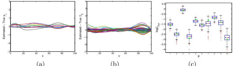
The residuals between the true and posterior mean over all components are displayed in Figure 2(a) and (b). Figure 2(c) compares the posterior samples of the elements σj2 of the residual covariance Σ0 to the true values. In Figure 3 we display a select set of plots of the true and posterior mean of components of µ(x) and Σ(x), along with the 95% highest posterior density intervals computed pointwise. From Figures 2 and 3, we see that we are clearly able to capture heteroscedasticity in combination with a nonparametric mean regression. The true values of the mean and covariance components are all contained within the 95% highest posterior density intervals, with these intervals typically narrow.
For the same simulated data set, we assessed predictive performance compared to ho-moscedastic models y ∼ Np(µ(x),Σ), with µj(x) either arising as independent GP(0, c)
0 20 40 60 80 100 −3
−2 −1 0 1 2 3
Mean
x
0 20 40 60 80 100
−3 −2 −1 0 1 2 3 4
Variance/Covariance
x
(a) (b)
Figure 1: Plot of each component of the (a) true mean vectorµ(x) and (b) true covariance matrix Σ(x) over X ={1, . . . ,100}.
0 20 40 60 80 100 −3
−2 −1 0 1 2 3
Estimated − True
µj
x 0 20 40 60 80 100
−3 −2 −1 0 1 2 3 4
Estimated − True
Σij
x
−4 −3.5 −3 −2.5 −2 −1.5 −1 −0.5 0 0.5
1 2 3 4 5 6 7 8 9 10
p
log
Σ0,p
(a) (b) (c)
Figure 2: Differences between each component of the true and posterior mean of (a) the meanµ(x), and (b) covariance Σ(x). The y-axis scale matches that of Figure 1. (c) Box plot of posterior samples of log(σj2) forj= 1, . . . , pcompared to the true value (green).
comparing to this latter homoscedastic model, we can directly analyze the benefits of our heteroscedastic model since both share exactly the same mean regression formulation. To generate a hold out sample, we removed 48 of the 1,000 observations by deleting observa-tionsyij with probabilitypi, where pi was chosen to vary withxi to slightly favor removal
in regions with more concentrated conditional response distributions.
We first calculated the average Kullback-Leibler divergence between the estimated and true predictive distribution of the missing elements yij given the observed elements of yi.
The average values were 0.341, 0.291 and 0.122 for the homoscedastic mean regression, ho-moscedastic latent factor mean regression and heteroscedastic latent factor mean regression, respectively. In this scenario, the missing observationsyij are imputed as an additional step
in the MCMC computations.1 The results clearly indicate that our Bayesian nonparamet-ric covariance regression model provides more accurate predictive distributions. We also observed improvements in estimating the meanµ(x) for the heteroscedastic approach.
1. Note that it is not necessary to impute the missingyijwithin our proposed Bayesian covariance regression
µ5(x)
Σ5,5(x) Σ1,2(x)
µ4(x)
Σ8,8(x)
Σ3,10(x)
µ9(x)
Σ9,9(x)
Σ7,9(x)
Figure 3: Plots of truth (red) and posterior mean (green) for select components of the mean µp(x) (left), variances Σpp(x) (middle), and covariances Σpq(x) (right).
The point-wise 95% highest posterior density intervals are shown in blue. The top row represents the component with the lowest L2 error between the truth and posterior mean. Likewise, the middle row represents median L2 error and the bottom row the worst L2 error. The size of the box indicates the relative magnitudes of each component.
In Case 2, we generated 30 replicates from a 30-dimensional parametric heteroscedastic model with y ∼Np(0,Σ(x)) and X ={1, . . . ,500}. To generate Σ(x), we chose a set of 5
evenly spaced knots xk and generated S(xk) ∼ N(0,Σs), with Σs =
P30
j=1sjs0j and sj ∼
N((−29,−27, . . . ,27,29)0, I30). The covariance is constructed as Σ(x) =αS˜(x) ˜S(x)0+ Σ0, x = 1, . . . ,500, where ˜S(x) is a spline fit to the S(xk) and Σ0 is a diagonal matrix with a N(0,1) truncated to be positive on its diagonal elements. The constantα is chosen to scale the maximum value ofαS˜(x) ˜S(x)0 to 1.
0 100 200 300 400 500 −2
−1 0 1 2 3 4
Variance/Covariance
x 0 100 200 300 400 500 0
0.5 1 1.5 2 2.5 3 3.5 4 4.5
Log Frobenius Norm Error
x
(a) (b)
0 100 200 300 400 500 −2
−1 0 1 2 3 4
Variance/Covariance
x
0 100 200 300 400 500 −2
−1 0 1 2 3 4
Variance/Covariance
x
(c) (d)
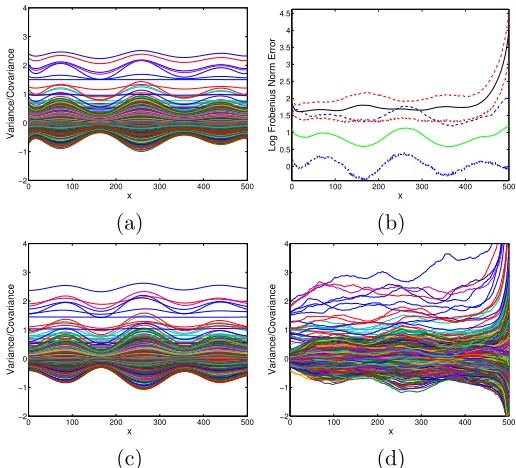
Figure 4: (a) Plot of each component of the true Σ(x) over X = {1, . . . ,500}; (c) cor-responding posterior means for our proposed approach; and (d) results for a Wishart discounting method, with (c)–(d) based on a single simulation replicate. (b) Mean and 95% highest posterior density intervals of the log Frobenius norm, log||Σ(τ,m)(x)−Σ(x)||2, for the proposed approach (blue and green) and Wishart discounting (red and black). Results are aggregated over 100 posterior samples and replicatesm= 1, . . . ,30.
5. Analysis of Spatio-temporal Trends in Flu
We now turn to our analysis of the Google Flu Trends data, described in detail in Section 5.1. Our focus is on applying our Bayesian nonparametric covariance regression model to capture the heteroscedasticity noted in the exploratory analysis of Appendix G. We also examine how our modeling approach is robust to (i) inaccuracies in the mean model, (ii) missing data, and (iii) outlying estimates.
For example, Duki´c et al. (2012) also examine portions of the Google Flu Trends data, but with the goal of on-line tracking of influenza rates on either a national, state, or regional level. Specifically, they employ a state-space model with particle learning. Our goal differs considerably. We aim to jointly analyze the full 183-dimensional data, as opposed to univari-ate modeling. Through such joint modeling, we can uncover important spatial dependencies lost when analyzing components of the data individually. Such spatial information can be key in predicting influenza rates based on partial observations from select regions or in retro-spectively imputing missing data. Additionally, the inherent redundancy and borrowing of information across locations provided by our model should lead to robustness to inaccuracies of flu estimates caused by malicious attacks to the Google infrastructure or unaccounted for sudden spikes in web searches (see Section 5.2.3). Hooten et al. (2010) consider the temporal dynamics of the state-level Google estimates, building on a susceptible–infected–recovered (SIR) model to capture the complexities of intra- and inter-state dynamics of flu disper-sal. Such a model aims to captures the intricate mechanistic structure of flu transmission, whereas our goals are focused primarily on fit using metrics such as predictive performance, with an eye towards scalability and robustness. Our exploratory data analysis of Appendix G shows that even with a very flexible and well-fit mean model, temporally changing spatial structure persist in the residuals motivating a heteroscedastic approach. In Section 4, we demonstrated that actually modeling such heteroscedasticity can improve predictive perfor-mance. Here, we show that the model of Section 2 can effectively capture such time-varying correlations in region-specific Google-estimated ILI rates, even when considering 183 regions jointly and in the presence of significant missing data.
5.1 Influenza Monitoring and Google Flu Trends
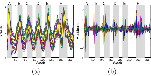
The surveillance of rates of influenza-like illness (ILI) within the United States is coordinated by the Centers for Disease Control and Prevention (CDC), which consolidates data from a large network of diagnostic laboratories, hospitals, clinics, individual healthcare providers, and state health departments. The CDC produces weekly reports (http://www.cdc.gov/ flu/weekly/) for 10 geographic regions and a U.S. aggregate rate. A plot of the number of isolates tested positive by the WHO and NREVSS from September 28, 2003 to October 24, 2010 is shown in Figure 5 (left). From these data and the CDC weekly flu reports, we defined a set of six events (Events A-F) corresponding to the 2003-2004, 2004-2005, 2005-2006, 2006-2007, 2007-2008, and 2009-2010 flu seasons, respectively. See the specific dates listed in Figure 5 (right). The 2003-2004 flu season began earlier than normal, and coincided with a flu vaccination shortage in many states. Additionally, the CDC found that the vaccination was “not effective or had very low effectiveness” (CDC, 2004). Finally, the 2009-2010 flu season coincides with the emergence of the 2009 H1N1 (“swine flu”) subtype in the U.S..
0 100 200 300 400 500 0
2000 4000 6000 8000 10000 12000 14000
Week
Number of Isolates
A(H1) A(H3) A(H1N1 2009) A(unk) A(sub not perf) B
Event Start Date End Date
A Sept. 28, 2003 Mar. 21, 2004 B Nov. 14, 2004 May 8, 2005 C Nov. 6, 2005 May 28, 2006 D Oct. 22, 2006 May 6, 2007 E Nov. 4, 2007 May 11, 2008 F Apr. 12, 2009 Feb. 7, 2010
Figure 5: Left: Number of isolates of Influenza A and B tested positive by the WHO and NREVSS over the period of September 29, 2003 to May 23, 2010, with Influenza A broken down into various subtypes. The green line indicates the time periods determined to be flu events. Right: Corresponding date ranges for flu events A-F.
models were fit to the weekly CDC ILI rates from 2003-2007. The fitted models are then used for making estimates in any region based on the ILI-related query rates from that region. A key advantage of the Google data is that the ILI rate predictions are available 1 to 2 weeks before the CDC weekly reports are published. Additionally, a user’s IP address is typically connected with a specific geographic area and can thus provide information at a finer scale than the 10-regional and U.S. aggregate reporting provided by the CDC.
There has, however, been significant recent debate about the accuracy of the Google Flu Trend estimates (Butler, 2013; Lazer et al., 2014; Harris, 2014). For this paper, we take a backseat in this discussion and simply use this data set to demonstrate the po-tential impact of our methods in this domain. Revised Google-estimated ILI rates could likewise be used in our framework, as could other recent sources of rapid ILI estimates, e.g., using Twitter data (Lamb et al., 2013; Achrekar et al., 2012) or platforms that in-corporate user-contributed reported cases (e.g.,https://flunearyou.org). Regardless, as we demonstrate in Section 5.2.3, our formulation provides some robustness to inaccurate estimates.
5.1.1 Data Description and Key Features
We analyze the Google Flu Trends data—produced on a weekly basis—from September 28, 2003 through October 24, 2010, totaling 370 weeks. These data provide ILI estimates in 183 regions, consisting of the U.S. national level, 50 states, 10 U.S. Department of Health & Human Services surveillance regions, and 122 cities. For our modeling, we take our observation vectors yi = (yi1, . . . , yip) to be the log of the Google-estimated ILI rates in
the p = 183 regions at week i. We denote the untransformed rates by ri = (ri1, . . . , rip).
Our predictor xi is simply a discrete time index indicating the current week (xi = i, i=
1, . . . ,370).
the estimated ILI rates for California and Los Angeles) that is naturally accommodated by a latent factor approach. Another important note is that there is substantial missing data with entire blocks of observations unavailable (as opposed to certain weeks sporadically being omitted). At the beginning of the examined time frame only 114 of the 183 regions were reporting. By the end of Year 1, there were 130 regions. These numbers increased to 173, 178, 180, and 183 by the end of Years 2, 3, 4, and 5, respectively.
5.2 Analysis via Bayesian Nonparametric Covariance Regression
We apply our Bayesian nonparametric covariance regression model as follows: logri ∼ N(µ(xi),Σ(xi)). Recall that ri simply stacks all region-specific measurements rij into
a 183-dimensional vector for each week xi. The spatial conditional correlation structure
at week xi is then captured by the covariance Σ(xi) = Θξ(xi)ξ(xi)0Θ0 + Σ0 and the mean by µ(xi) = Θξ(xi)ψ(xi). Temporal changes are implicitly modeled through the
proposed mean-covariance regression framework that allows for continuous variations in {µ(xi),Σ(xi)} via our Gaussian-process-based formulation. As such, we can also examine {µ(x),Σ(x)}for unobserved time pointsx∈ X occurring between the weekly measurements. We emphasize that our model does not explicitly encode any spatial structure between the regions (comprising the dimensions of the response vector yi), which is in contrast to many spatial and spatio-temporal models that build in a notion of neighborhood struc-ture. This is motivated both by the fact that, as we see in the correlation maps of the exploratory data analysis in Appendix G, the definition of “neighborhood” is not necessar-ily straightforward to encode using Euclidean distance since geographically distant regions might have significant correlation2. Likewise, this structure need not remain fixed across time. Finally, the full set of 183 regions—comprised of cities, states, regions, and the U.S. national level—represents a type of multiresolution spatial description of flu activ-ity. Although multiresolution-based spatial structures could be imposed based on known relationships, the inherent redundancy of these observations in this task is very well accom-modated by a latent factor model. As we have shown, such a structure is very simple to work with computationally and enables our ability to straightforwardly cope with missing data without imputing these values. We could consider a model that combines latent factor and neighborhood based approaches, leading to low-rank plus sparse precision forms for the covariance. This is a topic that has received considerable recent attention (Chandrasekaran et al., 2012). We leave this as a direction of future research.
Details on our model and MCMC setup are provided in Section 5.2.4.
5.2.1 Qualitative Assessment
We begin by producing correlation map snapshots similar to those of the exploratory data analysis in Appendix G, but here with an ability to examine instantaneous correlations that utilize (i) all 183 regions jointly and (ii) the entire time course. In contrast, the analysis of Appendix G reduces dimensionality to state-level, aggregates data amongst flu versus non-flu events to cope with data scarcity, and discards data prior to Event B due to significant missing values. The results presented in Figures 6 and 7 clearly demonstrate that
50 100 150 200 250 300 350 −5
0 5
Week
Means
F E D C B A
50 100 150 200 250 300 350
−0.2 0 0.2 0.4 0.6 0.8 1
Week
Correlations
F E D C B A
(a) (b)
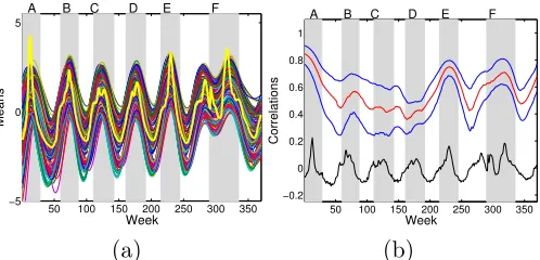
Figure 6: (a) Plot of posterior means of the nonparametric mean functionµj(x) for each of
the 183 Google Flu Trends regions. The thick yellow line indicates the empirical mean of the log Google-estimated ILI rates, logrij, across regionsj. (b) For New
York, the 25th, 50th, and 75th quantiles of correlation with the 182 other regions based on the posterior mean estimate of Σ(x). The black line is a scaled version of the log Google-estimated United States ILI rate. The shaded gray regions indicate the time periods determined to be flu events (see Figure 5).
we are able to capture temporal changes in the spatial correlations of the Google Flu Trends data, even in the presence of substantial missing information. In Figure 6(b), we plot the posterior mean of the 183 components of µ(x), showing trends that follow the empirical mean Google-estimated ILI rate. Although this mean model provides a slightly worse fit than the smoothing splines, our quantitative assessment of Section 5.2.2 demonstrates that modeling heteroscedasticity allows for a well-calibrated joint model. That is, we are robust to our simple choice for the mean regression function. (We note that more complicated mean models could be used within this framework, but this analysis demonstrates the flexibility of joint mean-covariance modeling.) For New York, in Figure 6(c) we plot the 25th, 50th, and 75th quantiles of correlation with the 182 other states and regions based on the posterior mean estimate of Σ(x). From this plot, we immediately notice the time-varying correlations.
New
Y
ork
California
Georgia
South
Dak
ota
February 2006 February 2007 February 2008 November 2009
Figure 7: For the states in Figure 12 and each of four key dates (February 2006 of Event C, February 2007 of Event D, February 2008 of Event E, and November 2009 of Event F), correlation maps based on the posterior mean estimate of Σ(x) using samples [5000 : 10 : 10000] from 10 chains. The color scale is exactly the same as in Figure 12. The plots indicate spatial structure captured by Σ(x), and that these spatial dependencies change over time. Note that no geographic information was included in our model.
provided in the Online Appendix.) This is enabled by the transfer of knowledge property described in Section 2.3. In particular, the row of Θ corresponding to South Dakota is informed by all of South Dakota’s available data while the latent GP basis elementsξ`k are
informed by all of the other regions’ data, in addition to assumed continuity of ξ`k which
shares information across time.
50 100 150 200 250 300 350 −5
0 5
Week
Means
F E D C B A
50 100 150 200 250 300 350
−5 0 5
Week
Means
F E D C B A
50 100 150 200 250 300 350
−5 0 5
Week
Means
F E D C B A
Large Bandwidth Matched Bandwidth Cross Validation Bandwidth
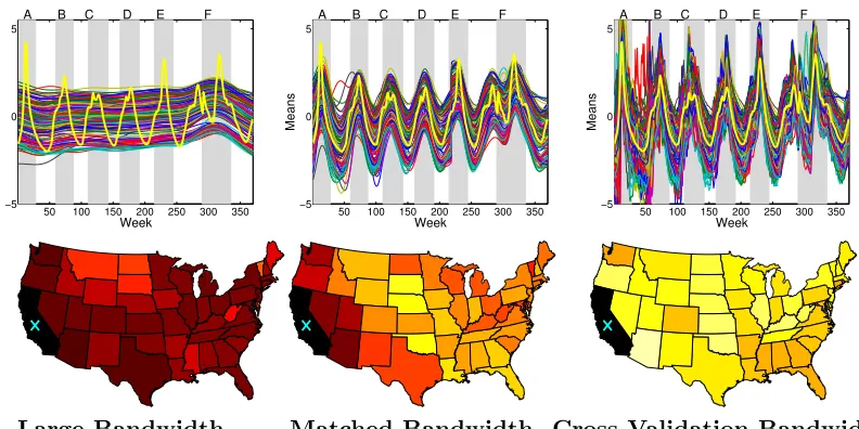
Figure 8: Top: Based on the nonparametric Nadaraya-Watson kernel estimator of Yin et al. (2010) using three different bandwidth settings ((κ/2)−1/2 = 0.07,0.02,0.0008), plots of the nonparametric mean estimate ˆµj(x) for each of
the 183 regions, as in Figure 6(b). The estimate is based on averaging samples [500 : 10 : 1000] from a stochastic EM chain that iterated between imputing missing values and computing the kernel estimate. Note that in the rightmost panel, the y-axis is truncated and the estimates in Event A actually extend to above 12. Bottom: Associated plots of correlations between California and all other states during February 2006 based on the nonparametric Nadaraya-Watson kernel estimator of the covariance function ˆΣ(x). The color scale is exactly the same as in Figures 12 and 7.
a lower-dimensional selection (or projection) of observations. For example, the common GARCH models cannot handle missing data and are limited to typically no more than 5 dimensions. On the other hand, our proposed algorithm can readily utilize all information available to model the heteroscedasticity present here.
missing values. In Figure 8(a), we see the unreasonably large mean values estimated at the beginning of the time series when there is substantial missing data. The smoothness of the mean function using a bandwidth of 0.02 captures the global changes in flu activity, leaving the covariance to explain the residual correlations in the observations, better matching our goals. However, the covariance, as visualized through the California correlation map of February 2006 (Figure 8(middle)), lacks key geographic structure such as the strong correlation between California and New York. This correlation is present during other flu events, and is unlikely to be truly missing from this event. Instead, the failure to capture this and other correlations is likely due to the increased uncertainty from the substantial early missing data and lack of global sharing of information. Using a much larger bandwidth of 0.07 necessarily leads to more sharing of information, and results in the presence of these correlations. The resulting over-smooth mean function, however, does not capture global flu variations. On the other hand, our Bayesian nonparametric method is able to maintain a local description of the data while sharing information across the entire time series, thus ameliorating sensitivity to missing data.
5.2.2 Model Calibration
The plots of Section 5.2.1 qualitatively demonstrate that we are able to capture time-varying changes in the spatial conditional correlation structure of the (log) Google-estimated ILI rates. Despite not encoding spatial structure in our latent-factor-based model, we note that some local geographic structure has emerged, while still allowing for long-range correlations and temporal changes in this structure. We now turn to a quantitative assessment of the fit and robustness of our model. To this end, we examine posterior predictive intervals of randomly heldout data. More specifically, from the available observations (omitting the significant number of truly missing observations), we randomly held out 10% of the values uniformly across time and regions. We then simulated from our Gibbs sampler treating these values as missing data and analytically marginalizing them from the complete data likelihood, just as we do for the truly missing values. Based on each of our MCMC samples, we formµ(x) and Σ(x) for eachx= 1, . . . ,370 and compute the predictive distribution for the heldout data given any available state-level observations at week x (i.e., we condition on a subset of observed regions, ignoring non-state-level measurements). Averaging over MCMC samples, we then form 95% posterior predictive intervals and associated coverage rates for eachx. We run this experiment of randomly holding out 10% of the observed data twice.
As a comparison, we consider an artificially generated homoscedastic model where we simply form ˆΣ = P370
i=1Σ(xi) for each of our MCMC samples. In this case, both models
compar-0.5 0.6 0.7 0.8 0.9 1 0.5
0.55 0.6 0.65 0.7 0.75 0.8 0.85 0.9 0.95 1
Hom. Coverage Rate
Het. Coverage Rate
1 1.1 1.2 1.3 1.4 1.5
1 1.1 1.2 1.3 1.4 1.5
Hom. Interval Length
Het. Interval Length
50 100 150 200 250 300 350
−0.6 −0.5 −0.4 −0.3 −0.2 −0.1 0 0.1 0.2 0.3
Week
Rate Difference
50 100 150 200 250 300 350
−0.25 −0.2 −0.15 −0.1 −0.05 0 0.05 0.1 0.15 0.2
Week
Interval Difference
Coverage Rates Interval Lengths
Figure 9: Comparison of posterior predictive intervals using our heteroscedastic model ver-sus a homoscedastic model. Top: Scatter plots of week-specific coverage rates and interval lengths, aggregated over two experiments. Bottom: Differences in coverage rates and interval lengths by week, separating the experiments via an offset for clarity.
ison, the artificially generated homoscedastic model had coverage rates of 93.7% and 93.8%, respectively. Importantly, the better calibrated coverage rates of our heteroscedastic model came from shorter predictive intervals with average lengths of 1.2272 and 1.2268 compared to 1.2469 and 1.2475 for the homoscedastic model.
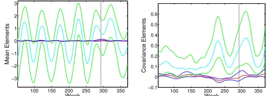
100 150 200 250 300 350 −3
−2 −1 0 1 2 3
Week
Mean Elements
100 150 200 250 300 350 −0.1
0 0.1 0.2 0.3 0.4 0.5 0.6
Week
Covariance Elements
Figure 10: Comparison of posterior mean estimates of µ(x) and Σ(x) using the full data versus using the data with the outlying weeks of April 26, 2009 and May 3, 2009 removed. Denote the resulting estimates by{µˆ(x),Σ(ˆ x)}and{µˆout(x),Σˆout(x)}, respectively. The two outlying weeks are highlighted by the gray shaded region. The blue lines indicate 0.05 and 0.95 pointwise-quantiles of the components (left) ˆ
µj(x)−µˆoutj (x) and (right) ˆΣij(x)−Σˆoutij (x). The red line is the median. The
green and cyan lines are the corresponding 0.05, 0.5, and 0.95 quantiles of the full data ˆµj(x) and ˆΣij(x) shown for scale. We omit the first year with significant
missing data to hone in on the smaller scale variability in subsequent years. No quantiles (blue/green lines) overlapped in this first year for the covariance elements, and trends were of the same scale for the mean elements.
5.2.3 Sensitivity to Outliers
As discussed in Section 5.1, there has been some debate about the accuracy of the Google Flu Trends estimates. In Cook et al. (2011), the two weeks of April 26, 2009 and May 3, 2009 were highlighted as having inflated Google estimates based on the significant media attention spurred by the H1N1 virus. In theory, our mean-covariance regression model has two defenses against such outliers. The first is due to the implicit shrinkage and regularization achieved through our use of a small set of latent basis functions. The second is the fact that an outlier at time x only has limited impact on inferences at time pointsx0 that are “far” from x. This is formalized by in Lemma 5, where we see that the covariance between Σij(x) and Σuv(x0) decays with (x−x0)2 (for univariate x and our squared exponential
kernelc(x, x0)).
5.2.4 MCMC Details, Sensitivity Analysis, and Convergence Diagnostics
We simulated 5 chains each for 10,000 MCMC iterations, discarded the first 5,000 for burn-in, and thinned the chains by examining every 10 samples. Each chain was initialized with parameters sampled from the prior. The hyperparameters were set as in the simulation study, except with larger truncation levels ¯L = 10 and ¯k = 20 and with the Gaussian process length-scale hyperparameter set to κψ = κ = 100 to account for the time scale
(weeks) and the rate at which ILI incidences change. By examining posterior samples of Θ, we found that the chosen truncation level was sufficiently large. To assess convergence, we performed the modified Gelman-Rubin diagnostic of Brooks and Gelman (1998) on the MCMC samples of the variance terms Σjj(xi). We also performed hyperparameter
sensitivity, letting κψ = κ = 200 to induce less temporal correlation and using a larger
truncation level of ¯L = ¯k = 20 with less stringent shrinkage hyperparameters a1 = a2 = 2 (instead of a1 = a2 = 10). The results were essentially identical to those presented. Note that after taking the log transformation, the data were preprocessed by removing the empirical mean of each region and scaling the entire data set by one over the largest variance of any of the 183 time series.
5.2.5 Computational Complexity
Each of our chains of 10,000 Gibbs iterations based on a naive implementation in MATLAB (R2010b) took approximately 12 hours on a machine with four Intel Xeon X5550 Quad-Core 2.67GHz processors and 48 GB of RAM. For a sense of scaling of computations, the p= 10,n= 100 simulation study of Section 4 took 10 minutes for 10,000 Gibbs iterations while the p= 30,n= 500 scenario of took 3 hours for 10,000 Gibbs iterations. In terms of memory and storage, our method only requires maintaining samples of a p×L matrix Θ, thep elements of Σ0, and anL×k×q×n matrix for the basis functions ξ(x). (Compare to maintaining thep×p×q×ndimensional matrix for the Nadaraya-Watson estimates of Σ(x) in the stochastic EM algorithm to which we compared.)
6. Discussion
multivariate data sets. In our Google Flu Trends analysis, we demonstrated the scalability, calibration, and robustness of our formulation.
There are many possible extensions of the proposed covariance regression framework. The most immediate are those that fall into the categories of (i) avoiding the multivariate Gaussian assumption, and (ii) scaling to data sets with larger numbers of observations.
In terms of (i), a natural possibility is to embed the proposed model within a richer hierarchical framework. For example, a promising approach is to use a Gaussian copula while allowing the marginal distributions to be unknown as in Hoff (2007). One can also use more flexible distributions for the latent variables and residuals, such as mixtures of Gaussians. Additionally, it would be trivial to extend our framework to accommodate mul-tivariate categorical responses, or joint categorical and continuous responses, by employing the latent variable probit model of Albert and Chib (1993).
In terms of (ii), our sampler relies on ¯Lׯk draws from an n-dimensional Gaussian (i.e., posterior draws of our Gaussian process random basis functions). For very large n, this becomes infeasible in practice since computations are, in general, O(n3). Standard tools for scaling up Gaussian process computation to large data sets, such as covariance tapering (Kaufman et al., 2008; Du et al., 2009) and the predictive process (Banerjee et al., 2008), can be applied directly in our context. Additionally, one might consider using the integrated nested Laplace approximations of Rue et al. (2009) for computations. One could also consider replacing the chosen basis elements with a basis expansion, wavelets, or simply autoregressive (i.e., band-limited) Gaussian processes. Including flat basis elements allows the model to collapse on homoscedasticity, enabling testing for heteroscedasticity.
It is also interesting to consider extensions that harness a known, predictor-independent structured covariance. One approach is to assume a low rank plus sparse model (instead of our low rank plus diagonal) in which the residuals have a sparse conditional dependence structure. For example, in the Google flu application the residuals could be modeled via a Markov random field to capture static local spatial dependencies while the low-rank portion captures time variation about this nominal structure. One could similarly extend to un-known sparse structures. Such formulations might allow for fewer latent factor dimensions. There are also a number of interesting theoretical directions related to showing posterior consistency and rates of convergence including in cases in which the dimensionp increases with sample size n.
Acknowledgments
Appendix A: Proofs of Theorems and Lemmas
In Lemma 7, we show that our proposed factorization of Σ(x) in (3) and (8) is sufficiently flexible to characterize any{Σ(x), x∈ X } for sufficiently largek. Let Xξ denote the space of all possibleL×k arrays ofX → <functions,XΣ0 all p×p diagonal matrices with non-negative entries, and XΘ all p×L real-valued matrices such that ΘΘ0 has finite elements. Recall that our modeling specification considers L→ ∞.
Lemma 7 Given Σ : X → P+
p , for sufficiently large k there exists {ξ(·),Θ,Σ0} ∈ Xξ⊗ XΘ⊗ XΣ0 such that Σ(x) = Θξ(x)ξ(x)0Θ0+ Σ0, for all x∈ X.
Proof Assume without loss of generality that Σ0 = 0p×p and take k≥p. Consider
Θ = [Ip 0p×1 0p×1 . . .], ξ(x) =
chol(Σ(x)) 0p×k−p
01×p 01×k−p
01×p 01×k−p ..
. ...
. (13)
Then, Σ(x) = Θξ(x)ξ(x)0ΘT for allx∈ X.
Proof [Proof of Theorem 2] Since X is compact, for every 0 > 0 there exists an open covering of 0-balls B0(x0) = {x : ||x−x0||2 < 0} with a finite subcover such that S
x0∈X0B0(x0)⊃ X, where|X0|=n. Then,
ΠΣ
sup
x∈X
||Σ(x)−Σ∗(x)||2<
= ΠΣ max x0∈X0
sup
x∈B0(x0)
||Σ(x)−Σ∗(x)||2<
!
. (14)
Define Z(x0) = supx∈B0(x0)||Σ(x)−Σ
∗(x)||
2. Since ΠΣ
max
x0∈X0
Z(x0)<
>0 ⇐⇒ ΠΣ(Z(x0)< )>0,∀x0 ∈ X0, (15) we only need to look at each0-ball independently, which we do as follows.
ΠΣ sup x∈B0(x0)
||Σ(x)−Σ∗(x)||2 <
!
≥ΠΣ
sup
x∈B0(x0)
||Σ∗(x0)−Σ∗(x)||2+ sup x∈B0(x0)
||Σ(x0)−Σ(x)||2
+||Σ(x0)−Σ∗(x0)||2<
≥ΠΣ sup x∈B0(x0)
||Σ∗(x0)−Σ∗(x)||2 < /3
!
·ΠΣ sup x∈B0(x0)
||Σ(x0)−Σ(x)||2 < /3
!
where the first inequality comes from repeated uses of the triangle inequality, and the second inequality follows from the fact that each of these terms is an independent event. We evaluate each of these terms in turn. The first follows directly from the assumed continuity of Σ∗(·). The second will follow from a statement of (almost sure) continuity of Σ(·) that arises from the (almost sure) continuity of theξ`k(·)∼GP(0, c) and the shrinkage prior on θ`k(i.e.,θ`k →0 almost surely as`→ ∞, and does so “fast enough”.) Finally, the third will
follow from the support of the conditionally Wishart prior on Σ(x0) at every fixedx0 ∈ X. Based on the continuity of Σ∗(·), for all/3>0 there exists an0,1 >0 such that
||Σ∗(x0)−Σ∗(x)||2< /3, ∀||x−x0||2 < 0,1. (17) Therefore, ΠΣ
supx∈B0,1(x0)||Σ
∗(x
0)−Σ∗(x)||2< /3
= 1.
Based on Theorem 8, each element of Λ(·) , Θξ(·) is almost surely continuous on X assumingk finite. Lettinggjk(x) = [Λ(x)]jk,
[Λ(x)Λ(x)0]ij = k
X
m=1
gim(x)gjm(x), ∀x∈ X. (18)
Eq. (18) represents a finite sum over pairwise products of almost surely continuous functions, and thus results in a matrix Λ(x)Λ(x)0 with elements that are almost surely continuous on X. Therefore, Σ(x) = Λ(x)Λ(x)0+ Σ0 = Θξ(x)ξ(x)0Θ0+ Σ0 is almost surely continuous on X. We can then conclude that for all /3>0 there exists an0,2>0 such that
ΠΣ sup x∈B0,2(x0)
||Σ(x0)−Σ(x)||2< /3
!
= 1. (19)
To examine the third term, we first note that
ΠΣ(||Σ(x0)−Σ∗(x0)||2< /3) = ΠΣ
||Θξ(x0)ξ(x0)0Θ0+ Σ0−Θ∗ξ∗(x0)ξ∗(x0)0Θ∗
0
−Σ∗0||2 < /3, (20) where{ξ∗(x0),Θ∗,Σ∗0}is any element ofXξ⊗XΘ⊗XΣ0 such that Σ
∗(x0) = Θ∗ξ∗(x0)ξ∗(x0)0Θ∗0
+ Σ∗0 with Θ∗ξ∗(x0)ξ∗(x0)0Θ∗
0
having rankk∗. Such a factorization exists by the assumption of Σ∗ being k∗-decomposable. Ifk∗ =p, Lemma 7 states that such a decomposition exists forany Σ∗. We can then bound this prior probability by
ΠΣ(||Σ(x0)−Σ∗(x0)||2< /3) ≥ΠΣ
||Θξ(x0)ξ(x0)0Θ0−Θ∗ξ∗(x0)ξ∗(x0)0Θ∗
0
||2 < /6 ΠΣ0(||Σ0−Σ
∗
0||2< /6) ≥ΠΣ
||Θξ(x0)ξ(x0)0Θ0−Θ∗ξ∗(x0)ξ∗(x0)0Θ∗
0
||2 < /6 ΠΣ0(||Σ0−Σ
∗
0||∞< /(6
√
p)), (21)
where the first inequality follows from the triangle inequality, and the second from the fact that for all A ∈ <p×p, ||A||
2 ≤ √
max1≤i≤pPpi=1|aij|. Since Σ0 = diag(σ12, . . . , σp2) with σ2i i.i.d.
∼ Ga(aσ, bσ), the support of
the gamma prior implies that
ΠΣ0(||Σ0−Σ
∗
0||∞< /(6
√
p)) = ΠΣ0
max 1≤i≤p|σ
2 i −σ
∗2
i |< /(6 √
π)
>0. (22)
Recalling that [ξ(x0)]`k=ξ`k(x0) withξ`k(x0) i.i.d.
∼ N(0,1) and taking Θ a real matrix with rank(Θ) =p,
Θξ(x0)ξ(x0)0Θ0|Θ∼W(k,ΘΘ0). (23) By Assumption 2.2, there is positive probability under ΠΘ on the set of Θ such that rank(Θ) = p. Since Θ∗ξ∗(x0)ξ∗(x0)0Θ∗0 is an arbitrary symmetric positive semidefinite matrix in<p×p with rankk≥k∗, and based on the support of the Wishart distribution,
ΠΣ
||Θξ(x0)ξ(x0)0Θ0−Θ∗ξ∗(x0)ξ∗(x0)0Θ∗0||2 < /6
>0. (24)
We thus conclude that ΠΣ(||Σ(x0)−Σ∗(x0)||2 < /3)>0.
For every Σ∗(·) and > 0, let 0 = min(0,1, 0,2) with 0,1 and 0,2 defined as above. Then, combining the positivity results of each of the three terms in Eq. (16) completes the proof.
Theorem 8 AssumingX compact, for every finitekandL→ ∞(orLfinite),Λ(·) = Θξ(·)
is almost surely continuous on X.
Proof [Proof of Theorem 8] We can represent each element of Λ(·) as follows:
[Λ(·)]jk = lim L→∞
θ11 θ12 . . . θ1L θ21 θ22 . . . θ2L
..
. ... . .. ... θp1 θp2 . . . θpL
ξ11(·) ξ12(·) . . . ξ1k(·) ξ21(·) ξ22(·) . . . ξ2k(·)
..
. ... . .. ... ξL1(·) ξL2(·) . . . ξLk(·)
jk = ∞ X `=1
θj`ξ`k(·). (25)
If ξ`k(x) is continuous for all `, k and sn(x) = Pn`=1θj`ξ`k(x) uniformly converges almost
surely to somegjk(x), thengjk(x) is almost surely continuous. That is, if for all >0 there
exists an N such that for alln≥N
Pr
sup
x∈X
|gjk(x)−sn(x)|<
= 1, (26)
thensn(x) converges uniformly almost surely to gjk(x) and we can conclude that gjk(x) is
continuous based on the definition of sn(x). To show almost sure uniform convergence, it
is sufficient to show that there exists anMn withP∞n=1Mnalmost surely convergent and
sup
x∈X
Letcnk = supx∈X|ξnk(x)|. Then,
sup
x∈X
|θjnξnk(x)| ≤ |θjn|cnk. (28)
Sinceξnk(·) i.i.d.
∼ GP(0, c) andX is compact, cnk <∞andE[cnk] = ¯cwith ¯cfinite. Defining Mn=|θjn|cnk,
EΘ,c " ∞ X n=1 Mn # =EΘ "
Ec|Θ
"∞ X
n=1
|θjn|cnk |Θ
##
=EΘ
"∞ X
n=1 |θjn|c¯
#
= ¯c
∞
X
n=1
EΘ[|θjn|], (29)
where the last equality follows from Fubini’s theorem. Based on Assumption 2.1, we con-clude thatE[P∞
n=1Mn]<∞ which implies that P∞n=1Mn converges almost surely.
Lemma 9 Assuming the prior specification of expression (9) with a2 >2 and γ > 2, the
rows of Θ are absolutely summable in expectation: P
`E(|θj`|) < ∞, satisfying Assump-tion 2.1.
Proof [Proof of Lemma 9] Recall that θj` ∼ N(0, φ−j`1τ`−1) with φj` ∼ Ga(γ/2, γ/2) and τ` =Q`h=1δh forδ1 ∼Ga(a1,1), δh ∼Ga(a2,1). Using the fact that if x ∼ N(0, σ2) then E[|x|] =σp2/πand ify∼Ga(a, b) then 1/y∼Inv-Ga(a,1/b) withE[1/y] = 1/(b·(a−1)), we derive that
∞
X
`=1
Eθ[|θj`|] =
∞
X
`=1
Eφ,τ[Eθ|φ,τ[|θj`| |φj`, τ`]] =
r 2 π ∞ X `=1
Eφ,τ[φ−j`1τ
−1 ` ] = r 2 π ∞ X `=1
Eφ[φ−j`1]Eτ[τ`−1] =
4 γ(γ−2)
r 2 π ∞ X `=1 Eδ " ` Y h=1 1 δh # = 1 a1−1
4 γ(γ −2)
r 2 π ∞ X `=1 1 a2−1
`−1
. (30)
When a2 >2 and γ >2, we conclude thatP
`E[|θj`|]<∞.
Proof[Proof of Lemma 4] Recall that Σ(x) = Θξ(x)ξ(x)0Θ0+Σ0with Σ0 = diag(σ12, . . . , σp2).
The elements of the respective matrices are independently distributed asθi`∼ N(0, φ−i`1τ`−1), ξ`k(·)∼GP(0, c), andσ−i 2 ∼Gamma(aσ, bσ). Letµσ and σ2σ represent the mean and
vari-ance of the implied inverse gamma prior onσ2i, respectively. In all of the following, we first condition on Θ and then use iterated expectations to find the marginal moments.
The expected covariance matrix at any predictor location x is simply derived as
E[Σ(x)] =E[E[Σ(x)|Θ]] =E[E[Θξ(x)ξ(x)0Θ0|Θ]] +µσIp =kE[ΘΘ0] +µσIp
= diag(kX `
φ−1`1τ`−1+µσ, . . . , k
X
`