Divide and Conquer Kernel Ridge Regression:
A Distributed Algorithm with Minimax Optimal Rates
Yuchen Zhang [email protected]
Department of Electrical Engineering and Computer Science University of California, Berkeley, Berkeley, CA 94720, USA
John Duchi [email protected]
Departments of Statistics and Electrical Engineering Stanford University, Stanford, CA 94305, USA
Martin Wainwright [email protected]
Departments of Statistics and Electrical Engineering and Computer Science University of California, Berkeley, Berkeley, CA 94720, USA
Editor:Hui Zou
Abstract
We study a decomposition-based scalable approach to kernel ridge regression, and show that it achieves minimax optimal convergence rates under relatively mild conditions. The method is simple to describe: it randomly partitions a dataset of size N into m subsets of equal size, computes an independent kernel ridge regression estimator for each subset using a careful choice of the regularization parameter, then averages the local solutions into a global predictor. This partitioning leads to a substantial reduction in computation time versus the standard approach of performing kernel ridge regression on allN samples. Our two main theorems establish that despite the computational speed-up, statistical op-timality is retained: as long asm is not too large, the partition-based estimator achieves the statistical minimax rate over all estimators using the set of N samples. As concrete examples, our theory guarantees that the number of subsets mmay grow nearly linearly for finite-rank or Gaussian kernels and polynomially inN for Sobolev spaces, which in turn allows for substantial reductions in computational cost. We conclude with experiments on both simulated data and a music-prediction task that complement our theoretical results, exhibiting the computational and statistical benefits of our approach.
Keywords: kernel ridge regression, divide and conquer, computation complexity
1. Introduction
In non-parametric regression, the statistician receives N samples of the form {(xi, yi)}Ni=1, where eachxi∈ X is a covariate andyi ∈R is a real-valued response, and the samples are drawn i.i.d. from some unknown joint distribution P overX ×R. The goal is to estimate a function fb: X → R that can be used to predict future responses based on observing
only the covariates. Frequently, the quality of an estimate fbis measured in terms of the
mean-squared prediction error E[(fb(X)−Y)2], in which case the conditional expectation
methods, known as regularizedM-estimators (van de Geer, 2000), are based on minimizing the combination of a data-dependent loss function with a regularization term. The focus of this paper is a popularM-estimator that combines the least-squares loss with a squared Hilbert norm penalty for regularization. When working in a reproducing kernel Hilbert space (RKHS), the resulting method is known as kernel ridge regression, and is widely used in practice (Hastie et al., 2001; Shawe-Taylor and Cristianini, 2004). Past work has established bounds on the estimation error for RKHS-based methods (Koltchinskii, 2006; Mendelson, 2002a; van de Geer, 2000; Zhang, 2005), which have been refined and extended in more recent work (e.g., Steinwart et al., 2009).
Although the statistical aspects of kernel ridge regression (KRR) are well-understood, the computation of the KRR estimate can be challenging for large datasets. In a standard implementation (Saunders et al., 1998), the kernel matrix must be inverted, which requires O(N3) time and O(N2) memory. Such scalings are prohibitive when the sample size N is large. As a consequence, approximations have been designed to avoid the expense of finding an exact minimizer. One family of approaches is based on low-rank approximation of the kernel matrix; examples include kernel PCA (Sch¨olkopf et al., 1998), the incomplete Cholesky decomposition (Fine and Scheinberg, 2002), or Nystr¨om sampling (Williams and Seeger, 2001). These methods reduce the time complexity to O(dN2) or O(d2N), where d N is the preserved rank. The associated prediction error has only been studied very recently. Concurrent work by Bach (2013) establishes conditions on the maintained rank that still guarantee optimal convergence rates; see the discussion in Section 7 for more detail. A second line of research has considered early-stopping of iterative optimization algorithms for KRR, including gradient descent (Yao et al., 2007; Raskutti et al., 2011) and conjugate gradient methods (Blanchard and Kr¨amer, 2010), where early-stopping provides regularization against over-fitting and improves run-time. If the algorithm stops after t iterations, the aggregate time complexity isO(tN2).
In this work, we study a different decomposition-based approach. The algorithm is ap-pealing in its simplicity: we partition the dataset of size N randomly into m equal sized subsets, and we compute the kernel ridge regression estimatefbi for each of thei= 1, . . . , m
subsets independently, with acareful choice of the regularization parameter. The estimates are then averaged via ¯f = (1/m)Pm
i=1fbi. Our main theoretical result gives conditions
under which the average ¯f achieves the minimax rate of convergence over the underlying Hilbert space. Even using naive implementations of KRR, this decomposition gives time and memory complexity scaling asO(N3/m2) andO(N2/m2), respectively. Moreover, our approach dovetails naturally with parallel and distributed computation: we are guaranteed superlinear speedup withmparallel processors (though we must still communicate the func-tion estimates from each processor). Divide-and-conquer approaches have been studied by several authors, including McDonald et al. (2010) for perceptron-based algorithms, Kleiner et al. (2012) in distributed versions of the bootstrap, and Zhang et al. (2013) for parametric smooth convex optimization problems. This paper demonstrates the potential benefits of divide-and-conquer approaches for nonparametric and infinite-dimensional regression prob-lems.
2001). An interesting consequence of our theoretical analysis is in demonstrating that, even though each partitioned sub-problem is based only on the fraction N/m of samples, it is nonetheless essential to regularize the partitioned sub-problems as though they had all N samples. Consequently, from a local point of view, each sub-problem is under-regularized. This “under-regularization” allows the bias of each local estimate to be very small, but it causes a detrimental blow-up in the variance. However, as we prove, the m-fold averaging underlying the method reduces variance enough that the resulting estimator ¯f still attains optimal convergence rate.
The remainder of this paper is organized as follows. We begin in Section 2 by providing background on the kernel ridge regression estimate and discussing the assumptions that underlie our analysis. In Section 3, we present our main theorems on the mean-squared error between the averaged estimate ¯f and the optimal regression function f∗. We provide both a result when the regression function f∗ belongs to the Hilbert space H associated with the kernel, as well as a more general oracle inequality that holds for a general f∗. We then provide several corollaries that exhibit concrete consequences of the results, including convergence rates ofr/N for kernels with finite rankr, and convergence rates ofN−2ν/(2ν+1) for estimation of functionals in a Sobolev space withν-degrees of smoothness. As we discuss, both of these estimation rates are minimax-optimal and hence unimprovable. We devote Sections 4 and 5 to the proofs of our results, deferring more technical aspects of the analysis to appendices. Lastly, we present simulation results in Section 6.1 to further explore our theoretical results, while Section 6.2 contains experiments with a reasonably large music prediction experiment.
2. Background and Problem Formulation
We begin with the background and notation required for a precise statement of our problem.
2.1 Reproducing Kernels
The method of kernel ridge regression is based on the idea of a reproducing kernel Hilbert space. We provide only a very brief coverage of the basics here, referring the reader to one of the many books on the topic (Wahba, 1990; Shawe-Taylor and Cristianini, 2004; Berlinet and Thomas-Agnan, 2004; Gu, 2002) for further details. Any symmetric and positive semidefinite kernel function K :X × X →R defines a reproducing kernel Hilbert space (RKHS for short). For a given distribution P on X, the Hilbert space is strictly contained inL2(P). For eachx∈ X, the functionz7→K(z, x) is contained with the Hilbert space H; moreover, the Hilbert space is endowed with an inner product h·,·iH such that K(·, x) acts as the representer of evaluation, meaning
hf, K(x,·)iH=f(x) forf ∈ H. (1) We let kgkH := p
hg, giH denote the norm in H, and similarly kgk2 := (R
X g(x)2dP(x))1/2
denotes the norm in L2(P). Under suitable regularity conditions, Mercer’s theorem guar-antees that the kernel has an eigen-expansion of the form
K(x, x0) =
∞ X
j=1
where µ1 ≥ µ2 ≥ · · · ≥ 0 are a non-negative sequence of eigenvalues, and {φj}∞j=1 is an orthonormal basis forL2(
P).
From the reproducing relation (1), we havehφj, φjiH= 1/µj for anyjandhφj, φj0iH = 0
for any j 6= j0. For any f ∈ H, by defining the basis coefficients θj = hf, φjiL2(
P) for j = 1,2, . . ., we can expand the function in terms of these coefficients as f = P∞j=1θjφj, and simple calculations show that
kfk22=
Z
X
f2(x)dP(x) =
∞ X
j=1
θj2, and kfk2H=hf, fiH=
∞ X
j=1 θ2j µj .
Consequently, we see that the RKHS can be viewed as an elliptical subset of the sequence space `2(N) as defined by the non-negative eigenvalues{µj}∞j=1.
2.2 Kernel Ridge Regression
Suppose that we are given a data set {(xi, yi)}Ni=1 consisting of N i.i.d. samples drawn from an unknown distribution P over X ×R, and our goal is to estimate the function that minimizes the mean-squared error E[(f(X)−Y)2], where the expectation is taken jointly over (X, Y) pairs. It is well-known that the optimal function is the conditional mean f∗(x) : = E[Y | X = x]. In order to estimate the unknown function f∗, we consider an M-estimator that is based on minimizing a combination of the least-squares loss defined over the dataset with a weighted penalty based on the squared Hilbert norm,
b
f := argmin f∈H
1 N
N
X
i=1
(f(xi)−yi)2+λkfk2H
, (2)
whereλ >0 is a regularization parameter. When His a reproducing kernel Hilbert space, then the estimator (2) is known as the kernel ridge regression estimate, or KRR for short. It is a natural generalization of the ordinary ridge regression estimate (Hoerl and Kennard, 1970) to the non-parametric setting.
By the representer theorem for reproducing kernel Hilbert spaces (Wahba, 1990), any solution to the KRR program (2) must belong to the linear span of the kernel functions {K(·, xi), i = 1, . . . , N}. This fact allows the computation of the KRR estimate to be reduced to an N-dimensional quadratic program, involving the N2 entries of the kernel matrix{K(xi, xj), i, j = 1, . . . , n}. On the statistical side, a line of past work (van de Geer, 2000; Zhang, 2005; Caponnetto and De Vito, 2007; Steinwart et al., 2009; Hsu et al., 2012) has provided bounds on the estimation error offbas a function of N and λ.
3. Main Results and Their Consequences
the estimation error in this case. Both of these theorems apply to any trace class kernel, but as we illustrate, they provide concrete results when applied to specific classes of kernels. Indeed, as a corollary, we establish that our distributed KRR algorithm achieves minimax-optimal rates for three different kernel classes, namely finite-rank, Gaussian, and Sobolev.
3.1 Algorithm and Assumptions
The divide-and-conquer algorithm Fast-KRR is easy to describe. Rather than solving the kernel ridge regression problem (2) on all N samples, the Fast-KRR method executes the following three steps:
1. Divide the set of samples {(x1, y1), . . . ,(xN, yN)} evenly and uniformly at random into themdisjoint subsetsS1, . . . , Sm⊂ X ×R, such that every subset containsN/m samples.
2. For eachi= 1,2, . . . , m, compute thelocal KRR estimate
b
fi:= argmin f∈H
1 |Si|
X
(x,y)∈Si
(f(x)−y)2+λkfk2H
. (3)
3. Average together the local estimates and output ¯f = m1 Pm
i=1fbi.
This description actually provides a family of estimators, one for each choice of the regular-ization parameter λ >0. Our main result applies to any choice ofλ, while our corollaries for specific kernel classes optimize λas a function of the kernel.
We now describe our main assumptions. Our first assumption, for which we have two variants, deals with the tail behavior of the basis functions{φj}∞
j=1.
Assumption A For some k ≥2, there is a constant ρ < ∞ such that E[φj(X)2k] ≤ ρ2k for all j∈N.
In certain cases, we show that sharper error guarantees can be obtained by enforcing a stronger condition of uniform boundedness.
Assumption A0 There is a constant ρ <∞ such thatsupx∈X|φj(x)| ≤ρ for all j∈N. Assumption A0 holds, for example, when the input x is drawn from a closed interval and the kernel is translation invariant, i.e.K(x, x0) =ψ(x−x0) for some even functionψ. Given input spaceX and kernelK, the assumption is verifiable without the data.
Recalling that f∗(x) : = E[Y |X = x], our second assumption involves the deviations of the zero-mean noise variablesY −f∗(x). In the simplest case, whenf∗ ∈ H, we require only a bounded variance condition:
Assumption B The function f∗∈ H, and forx∈ X, we have E[(Y −f∗(x))2 |x]≤σ2. When the function f∗ 6∈ H, we require a slightly stronger variant of this assumption. For each λ≥0, define
fλ∗= argmin f∈H
n
E(f(X)−Y)2+λkfk2H o
Note that f∗ = f0∗ corresponds to the usual regression function. As f∗ ∈ L2(P), for each λ≥0, the associated mean-squared error σλ2(x) :=E[(Y −fλ∗(x))2 |x] is finite for almost everyx. In this more general setting, the following assumption replaces Assumption B: Assumption B0 For any λ≥0, there exists a constantτλ<∞ such thatτλ4 =E[σλ4(X)]. 3.2 Statement of Main Results
With these assumptions in place, we are now ready for the statements of our main results. All of our results give bounds on the mean-squared estimation errorE[kf¯−f∗k22] associated with the averaged estimate ¯fbased on an assigningn=N/msamples to each ofmmachines. Both theorem statements involve the following three kernel-related quantities:
tr(K) :=
∞ X
j=1
µj, γ(λ) :=
∞ X
j=1 1 1 +λ/µj
, and βd=
∞ X
j=d+1
µj. (5)
The first quantity is the kernel trace, which serves a crude estimate of the “size” of the kernel operator, and assumed to be finite. The second quantityγ(λ), familiar from previous work on kernel regression (Zhang, 2005), is the effective dimensionality of the kernel K with respect toL2(P). Finally, the quantity βd is parameterized by a positive integer dthat we may choose in applying the bounds, and it describes the tail decay of the eigenvalues ofK. Ford= 0, note that β0 = trK. Finally, both theorems involve a quantity that depends on the number of momentsk in Assumption A:
b(n, d, k) := max
p
max{k,log(d)},max{k,log(d)} n1/2−1/k
. (6) Here the integer d ∈N is a free parameter that may be optimized to obtain the sharpest possible upper bound. (The algorithm’s execution is independent of d.)
Theorem 1 With f∗∈ H and under Assumptions A and B, the mean-squared error of the averaged estimate f¯is upper bounded as
E
h f¯−f∗
2 2
i
≤
8 +12 m
λkf∗k2H+ 12σ 2γ(λ) N + infd∈N
T1(d) +T2(d) +T3(d) , (7) where
T1(d) =
8ρ4kf∗k2Htr(K)βd
λ , T2(d) =
4kf∗k2H+ 2σ2/λ m
µd+1+
12ρ4tr(K)βd λ
, and
T3(d) =
Cb(n, d, k)ρ 2γ(λ)
√ n
k
µ0kf∗k2H 1 +
2σ2 mλ +
4kf∗k2
H
m
!
,
and C denotes a universal (numerical) constant.
Before doing so, let us make a few heuristic arguments in order to provide intuition. In typical settings, the term T3(d) goes to zero quickly: if the number of moments k is suitably large and number of partitions m is small—say enough to guarantee that (b(n, d, k)γ(λ)/√n)k = O(1/N)—it will be of lower order. As for the remaining terms, at a high level, we show that an appropriate choice of the free parameterdleaves the first two terms in the upper bound (7) dominant. Note that the termsµd+1 and βd are decreas-ing in d while the term b(n, d, k) increases with d. However, the increasing term b(n, d, k) grows only logarithmically in d, which allows us to choose a fairly large value without a significant penalty. As we show in our corollaries, for many kernels of interest, as long as the number of machines m is not “too large,” this tradeoff is such that T1(d) and T2(d) are also of lower order compared to the two first terms in the bound (7). In such settings, Theorem 1 guarantees an upper bound of the form
E
h
f¯−f∗
2 2
i
=O(1)·h λkf∗k2H
| {z }
Squared bias + σ
2γ(λ) N
| {z }
Variance
i
. (8)
This inequality reveals the usual bias-variance trade-off in non-parametric regression; choos-ing a smaller value of λ >0 reduces the first squared bias term, but increases the second variance term. Consequently, the setting ofλthat minimizes the sum of these two terms is defined by the relationship
λkf∗k2H ' σ2γ(λ)
N . (9) This type of fixed point equation is familiar from work on oracle inequalities and local com-plexity measures in empirical process theory (Bartlett et al., 2005; Koltchinskii, 2006; van de Geer, 2000; Zhang, 2005), and when λis chosen so that the fixed point equation (9) holds this (typically) yields minimax optimal convergence rates (Bartlett et al., 2005; Koltchin-skii, 2006; Zhang, 2005; Caponnetto and De Vito, 2007). In Section 3.3, we provide detailed examples in which the choiceλ∗ specified by equation (9), followed by application of The-orem 1, yields minimax-optimal prediction error (for the Fast-KRR algorithm) for many kernel classes.
We now turn to an error bound that applies without requiring thatf∗ ∈ H. In order to do so, we introduce an auxiliary variable ¯λ∈[0, λ] for use in our analysis (the algorithm’s execution does not depend on ¯λ, and in our ensuing bounds we may choose any ¯λ∈[0, λ] to give the sharpest possible results). Let the radius R = f¯∗
λ
H, where the population
(regularized) regression functionf¯λ∗ was previously defined (4). The theorem requires a few additional conditions to those in Theorem 1, involving the quantities tr(K), γ(λ) and βd defined in Eq. (5), as well as the error moment τ¯λ from Assumption B0. We assume that the triplet (m, d, k) of positive integers satisfy the conditions
βd≤
λ (R2+τ2
¯ λ/λ)N
, µd+1≤
1 (R2+τ2
¯ λ/λ)N
,
m≤min
( √
N ρ2γ(λ) log(d),
N1−k2
(R2+τ2 ¯ λ/λ)
2/k(b(n, d, k)ρ2γ(λ))2
)
.
We then have the following result:
Theorem 2 Under condition (10), Assumption A with k≥4, and Assumption B0, for any ¯
λ∈[0, λ]and q >0 we have
E
h
f¯−f∗
2 2
i
≤
1 +1 q
inf
kfkH≤R
kf−f∗k22+ (1 +q)EN,m(λ,λ, R, ρ)¯ (11) where the residual term is given by
EN,m(λ,¯λ, R, ρ) : =
4 + C m
(λ−λ)R¯ 2+Cγ(λ)ρ 2τ2
¯ λ N +
C N
, (12) and C denotes a universal (numerical) constant.
Remarks: Theorem 2 is an oracle inequality, as it upper bounds the mean-squared error in terms of the error inf
kfkH≤R
kf−f∗k2
2, which may only be obtained by an oracle knowing the sampling distributionP, along with the residual error term (12).
In some situations, it may be difficult to verify Assumption B0. In such scenarios, an alternative condition suffices. For instance, if there exists a constant κ < ∞ such that E[Y4] ≤ κ4, then under condition (10), the bound (11) holds with τ¯λ2 replaced by
p
8 tr(K)2R4ρ4+ 8κ4—that is, with the alternative residual error
e
EN,m(λ,¯λ, R, ρ) : =
2 + C m
(λ−λ)R¯ 2+Cγ(λ)ρ 2p
8 tr(K)2R4ρ4+ 8κ4 N +
C N
. (13) In essence, if the response variableY has sufficiently many moments, the prediction mean-square error τ¯λ2 in the statement of Theorem 2 can be replaced by constants related to the size of f¯∗
λ
H. See Section 5.2 for a proof of inequality (13).
In comparison with Theorem 1, Theorem 2 provides somewhat looser bounds. It is, however, instructive to consider a few special cases. For the first, we may assume that f∗ ∈ H, in which case kf∗kH <∞. In this setting, the choice ¯λ= 0 (essentially) recovers Theorem 1, since there is no approximation error. Taking q→0, we are thus left with the bound
Ekf¯−f∗k22] . λkf∗k2H+
γ(λ)ρ2τ02
N , (14) where . denotes an inequality up to constants. By inspection, this bound is roughly equivalent to Theorem 1; see in particular the decomposition (8). On the other hand, when the conditionf∗∈ Hfails to hold, we can take ¯λ=λ, and then chooseqto balance between the familiar approximation and estimation errors: we have
E[kf¯−f∗k22].
1 +1 q
inf
kfkH≤R
kf −f∗k22
| {z }
approximation
+ (1 +q)
γ(λ)ρ2τ2 λ N
| {z }
estimation
. (15)
when ignoring constants and logarithm terms, the quantitymmay grow at ratepN/γ2(λ). By contrast, Theorem 1 allows m to grow as quickly as N/γ2(λ) (recall the remarks on T3(d) following Theorem 1 or look ahead to condition (28)). Thus—at least in our current analysis—generalizing to the case thatf∗6∈ H prevents us from dividing the data into finer subsets.
3.3 Some Consequences
We now turn to deriving some explicit consequences of our main theorems for specific classes of reproducing kernel Hilbert spaces. In each case, our derivation follows the broad outline given the the remarks following Theorem 1: we first choose the regularization parameterλ to balance the bias and variance terms, and then show, by comparison to known minimax lower bounds, that the resulting upper bound is optimal. Finally, we derive an upper bound on the number of subsampled data setsm for which the minimax optimal convergence rate can still be achieved. Throughout this section, we assume that f∗ ∈ H.
3.3.1 Finite-rank Kernels
Our first corollary applies to problems for which the kernel has finite rank r, meaning that its eigenvalues satisfy µj = 0 for all j > r. Examples of such finite rank kernels include the linear kernelK(x, x0) =hx, x0i
Rd, which has rank at mostr=d; and the kernel
K(x, x) = (1+x x0)mgenerating polynomials of degreem, which has rank at mostr=m+1.
Corollary 3 For a kernel with rankr, consider the output of the Fast-KRR algorithm with λ=r/N. Suppose that Assumption B and Assumptions A (or A0) hold, and that the number of processors m satisfy the bound
m≤c N
k−4
k−2
r2kk−−12ρ 4k k−2 log
k k−2 r
(Assumption A) or m≤c N
r2ρ4logN (Assumption A
0),
where c is a universal (numerical) constant. For suitably large N, the mean-squared error is bounded as
E
h
f¯−f∗
2 2
i
=O(1)σ 2r
N . (16) For finite-rank kernels, the rate (16) is known to be minimax-optimal, meaning that there is a universal constantc0 >0 such that
inf
e
f sup
kf∗k H≤1
E[kfe−f∗k22]≥c0
r
N, (17) where the infimum ranges over all estimatorsfebased on observing allN samples (and with
3.3.2 Polynomially Decaying Eigenvalues
Our next corollary applies to kernel operators with eigenvalues that obey a bound of the form
µj ≤C j−2ν for all j= 1,2, . . ., (18) where C is a universal constant, and ν > 1/2 parameterizes the decay rate. We note that equation (5) assumes a finite kernel trace tr(K) := P∞j=1µj. Since tr(K) appears in Theorem 1, it is natural to useP∞j=1Cj−2ν as an upper bound on tr(K). This upper bound is finite if and only ifν >1/2.
Kernels with polynomial decaying eigenvalues include those that underlie for the Sobolev spaces with different orders of smoothness (e.g. Birman and Solomjak, 1967; Gu, 2002). As a concrete example, the first-order Sobolev kernel K(x, x0) = 1 + min{x, x0} generates an RKHS of Lipschitz functions with smoothness ν = 1. Other higher-order Sobolev kernels also exhibit polynomial eigendecay with larger values of the parameter ν.
Corollary 4 For any kernel with ν-polynomial eigendecay (18), consider the output of the Fast-KRR algorithm with λ= (1/N)2ν2+1ν . Suppose that Assumption B and Assumption A
(or A0) hold, and that the number of processors satisfy the bound
m≤c N
2(k−4)ν−k
(2ν+1)
ρ4klogkN
!k−12
(Assumption A) or m≤c N
2ν−1 2ν+1
ρ4logN (Assumption A
0),
where c is a constant only depending on ν. Then the mean-squared error is bounded as
E
h
f¯−f∗
2 2
i
=O
σ2
N
2ν2+1ν
. (19) The upper bound (19) is unimprovable up to constant factors, as shown by known minimax bounds on estimation error in Sobolev spaces (Stone, 1982; Tsybakov, 2009); see also Theorem 2(b) of Raskutti et al. (2012).
3.3.3 Exponentially Decaying Eigenvalues
Our final corollary applies to kernel operators with eigenvalues that obey a bound of the form
µj ≤c1 exp(−c2j2) for all j= 1,2, . . ., (20) for strictly positive constants (c1, c2). Such classes include the RKHS generated by the Gaussian kernel K(x, x0) = exp(−kx−x0k22).
Corollary 5 For a kernel with sub-Gaussian eigendecay (20), consider the output of the Fast-KRR algorithm withλ= 1/N. Suppose that Assumption B and Assumption A (or A0) hold, and that the number of processors satisfy the bound
m≤c N
k−4
k−2
ρk4−k2 log 2k−1
k−2 N
(Assumption A) or m≤c N
ρ4log2N (Assumption A
where c is a constant only depending on c2. Then the mean-squared error is bounded as
E
h
f¯−f∗
2 2
i
=O
σ2 √
logN N
. (21)
The upper bound (21) is minimax optimal; see, for example, Theorem 1 and Example 2 of the recent paper by Yang et al. (2015).
3.3.4 Summary
Each corollary gives a critical threshold for the numbermof data partitions: as long asmis below this threshold, the decomposition-based Fast-KRR algorithm gives the optimal rate of convergence. It is interesting to note that the number of splits may be quite large: each grows asymptotically with N whenever the basis functions have more than four moments (viz. Assumption A). Moreover, the Fast-KRR method can attain these optimal conver-gence rates while using substantially less computation than standard kernel ridge regression methods, as it requires solving problems only of sizeN/m.
3.4 The Choice of Regularization Parameter
In practice, the local sample size on each machine may be different and the optimal choice for the regularizationλmay not be known a priori, so that an adaptive choice of the regu-larization parameterλis desirable (e.g. Tsybakov, 2009, Chapters 3.5–3.7). We recommend using cross-validation to choose the regularization parameter, and we now sketch a heuristic argument that an adaptive algorithm using cross-validation may achieve optimal rates of convergence. (We leave fuller analysis to future work.)
Letλnbe the (oracle) optimal regularization parameter given knowledge of the sampling distributionP and eigen-structure of the kernel K. We assume (cf. Corollary 4) that there is a constant ν >0 such thatλnn−ν asn→ ∞. Letni be the local sample size for each machineiandN the global sample size; we assume thatni
√
N (clearly,N ≥ni). First, use local cross-validation to choose regularization parametersbλni and bλn2
i/N corresponding
to samples of sizeni and n2i/N, respectively. Heuristically, if cross validation is successful, we expect to havebλni 'n−i ν and λbn2
i/N 'N
νn−2ν
i , yielding that bλ2n
i/bλn2i/N 'N
−ν. With
this intuition, we then compute local estimates
b
fi:= argmin f∈H
1 ni
X
(x,y)∈Si
(f(x)−y)2+λb(i)kfk2H where bλ(i):= b
λ2ni
b
λn2
i/N
(22)
and global average estimate ¯f = Pm
i=1nNifbi as usual. Notably, we have bλ(i) 'λN in this
heuristic setting. Using formula (22) and the average ¯f, we have
E
h
f¯−f∗
2 2
i
=E
m
X
i=1 ni N
b
fi−E[fbi]
2 2
+
m
X
i=1 ni N
E[fbi]−f∗
2 2 ≤
m
X
i=1 n2i N2E
h
bfi−E[fbi]
2 2
i
+ max i∈[m]
n
E[fbi]−f∗
2 2
o
Using Lemmas 6 and 7 from the proof of Theorem 1 to come and assuming thatλbn is
con-centrated tightly enough around λn, we obtainkE[fbi]−f∗k22 =O(λNkf∗k2H) by Lemma 6
and thatE[kfbi−E[fbi]k22] =O(γ(λN)
ni ) by Lemma 7. Substituting these bounds into
inequal-ity (23) and noting that P
ini = N, we may upper bound the overall estimation error as
E
h f¯−f∗
2 2
i
≤ O(1)·
λNkf∗k2H+
γ(λN) N
.
While the derivation of this upper bound was non-rigorous, we believe that it is roughly accurate, and in comparison with the previous upper bound (8), it provides optimal rates of convergence.
4. Proofs of Theorem 1 and Related Results
We now turn to the proofs of Theorem 1 and Corollaries 3 through 5. This section con-tains only a high-level view of proof of Theorem 1; we defer more technical aspects to the appendices.
4.1 Proof of Theorem 1
Using the definition of the averaged estimate ¯f = m1 Pm
i=1fbi, a bit of algebra yields
E[f¯−f∗
2 2] =E[
( ¯f−E[ ¯f]) + (E[ ¯f]−f∗)
2 2] =E[f¯−E[ ¯f]
2 2] +
E[ ¯f]−f∗
2
2+ 2E[hf¯−E[ ¯f],E[ ¯f]−f
∗i
L2(
P)]
=E
1 m
m
X
i=1
(fbi−E[fbi])
2 2
+E[ ¯f]−f∗
2 2,
where we used the fact that E[fbi] = E[ ¯f] for each i ∈ [m]. Using this unbiasedness once
more, we bound the variance of the terms fbi−E[ ¯f] to see that
E
h
f¯−f∗
2 2
i
= 1 mE
h
kfb1−E[fb1]k22 i
+kE[fb1]−f∗k22
≤ 1 mE
h
kfb1−f∗k22 i
+kE[fb1]−f∗k22, (24)
where we have used the fact thatE[fbi] minimizesE[kfbi−fk22] overf ∈ H.
The error bound (24) suggests our strategy: we upper boundE[kf1b−f∗k22] andkE[f1b]−
f∗k2
2 respectively. Based on equation (3), the estimate f1b is obtained from a standard
kernel ridge regression with sample size n=N/m and ridge parameterλ. Accordingly, the following two auxiliary results provide bounds on these two terms, where the reader should recall the definitions of b(n, d, k) and βd from equation (5). In each lemma,C represents a universal (numerical) constant.
Lemma 6 (Bias bound) Under Assumptions A and B, for each d= 1,2, . . ., we have
kE[fb]−f∗k22≤8λkf∗k2H+
8ρ4kf∗k2
Htr(K)βd λ +
Cb(n, d, k)ρ 2γ(λ)
√ n
k
Lemma 7 (Variance bound) Under Assumptions A and B, for each d = 1,2, . . ., we have
E[kfb−f∗k22]≤12λkf∗k2H+
12σ2γ(λ) n +
2σ2 λ + 4kf
∗k2
H
µd+1+
12ρ4tr(K)βd λ +
Cb(n, d, k)ρ 2γ(λ)
√ n
k
kf∗k22
!
. (26)
The proofs of these lemmas, contained in Appendices A and B respectively, constitute one main technical contribution of this paper. Given these two lemmas, the remainder of the theorem proof is straightforward. Combining the inequality (24) with Lemmas 6 and 7 yields the claim of Theorem 1.
Remarks: The proofs of Lemmas 6 and 7 are somewhat complex, but to the best of our knowledge, existing literature does not yield significantly simpler proofs. We now discuss this claim to better situate our technical contributions. Define the regularized population minimizerfλ∗:= argminf∈H{E[(f(X)−Y)2] +λkfk2H}. Expanding the decomposition (24)
of the L2(P)-risk into bias and variance terms, we obtain the further bound E
h
f¯−f∗
2 2
i
≤ kE[fb1]−f∗k22+
1 mE
h
kfb1−f∗k22 i
=kE[fb1]−f∗k22
| {z }
:=T1
+1 m
kfλ∗−f∗k2 2
| {z }
:=T2
+E
h
kfb1−f∗k22 i
− kfλ∗−f∗k22
| {z }
:=T3
=T1+ 1
m(T2+T3).
In this decomposition, T1 and T2 are bias and approximation error terms induced by the regularization parameterλ, whileT3is an excess risk (variance) term incurred by minimizing the empirical loss.
This upper bound illustrates three trade-offs in our subsampled and averaged kernel regression procedure:
• The trade-off between T2 and T3: when the regularization parameter λ grows, the bias term T2 increases while the variance termT3 converges to zero.
• The trade-off between T1 and T3: when the regularization parameter λ grows, the bias term T1 increases while the variance termT3 converges to zero.
• The trade-off between T1 and the computation time: when the number of machines mgrows, the bias termT1 increases (as the local sample sizen=N/mshrinks), while the computation time N3/m2 decreases.
Theoretical results in the KRR literature focus on the trade-off betweenT2 and T3, but in the current context, we also need an upper bound on the bias termT1, which is not relevant for classical (centralized) analyses.
With this setting in mind, Lemma 6 tightly upper bounds the bias T1 as a function of λand n. An essential part of the proof is to characterize the properties ofE[fb1], which is
literature on this problem, and the proof of Lemma 6 introduces novel techniques for this purpose.
On the other hand, Lemma 7 upper bounds E[kfb1−f∗k22] as a function of λ and n.
Past work has focused on bounding a quantity of this form, but for technical reasons, most work (e.g. van de Geer, 2000; Mendelson, 2002b; Bartlett et al., 2002; Zhang, 2005) focuses on analyzing the constrained form
b
fi := argmin
kfkH≤C
1 |Si|
X
(x,y)∈Si
(f(x)−y)2, (27)
of kernel ridge regression. While this problem traces out the same set of solutions as that of the regularized kernel ridge regression estimator (3), it is non-trivial to determine a matched setting of λ for a given C. Zhang (2003) provides one of the few analyses of the regularized ridge regression estimator (3) (or (2)), providing an upper bound of the form
E[kfb−f∗k22] = O(λ+ 1/λn ), which is at best O(√1
n). In contrast, Lemma 7 gives upper boundO(λ+γ(nλ)); the effective dimensionγ(λ) is often much smaller than 1/λ, yielding a stronger convergence guarantee.
4.2 Proof of Corollary 3
We first present a general inequality bounding the size ofm for which optimal convergence rates are possible. We assume that dis chosen large enough such that we have log(d)≥k and d≥N. In the rest of the proof, our assignment to dwill satisfy these inequalities. In this case, inspection of Theorem 1 shows that if m is small enough that
s
logd N/mρ
2γ(λ)
!k
1 mλ ≤
γ(λ) N ,
then the term T3(d) provides a convergence rate given by γ(λ)/N. Thus, solving the ex-pression above form, we find
mlogd N ρ
4γ(λ)2= λ2/km2/kγ(λ)2/k
N2/k or m
k−2
k = λ
2
kN k−2
k
γ(λ)2k−k1ρ4logd
.
Taking (k−2)/k-th roots of both sides, we obtain that if
m≤ λ
2
k−2N
γ(λ)2kk−−12ρ 4k k−2 log
k k−2 d
, (28)
then the term T3(d) of the bound (7) is O(γ(λ)/N).
Now we apply the bound (28) in the case in the corollary. Let us take d= max{r, N}. Notice thatβd =βr =µr+1= 0. We find that γ(λ)≤r since each of its terms is bounded by 1, and we takeλ=r/N. Evaluating the expression (28) with this value, we arrive at
m≤ N
k−4
k−2
r2kk−−12ρ 4k k−2 log
k k−2 d
If we have sufficiently many moments thatk≥logN, andN ≥r (for example, if the basis functionsφj have a uniform boundρ, thenkcan be chosen arbitrarily large), then we may take k= logN, which implies that Nkk−−42 = Ω(N),r2
k−1
k−2 =O(r2) and ρ 4k
k−2 =O(ρ4) ; and
we replace logdwith logN. Then so long as m≤c N
r2ρ4logN for some constantc >0, we obtain an identical result. 4.3 Proof of Corollary 4
We follow the program outlined in our remarks following Theorem 1. We must first choose λon the order ofγ(λ)/N. To that end, we note that setting λ=N−2ν2+1ν gives
γ(λ) =
∞ X
j=1
1
1 +j2νN−2ν2+1ν
≤N2ν1+1 + X
j>N2ν1+1
1
1 +j2νN−2ν2+1ν
≤N2ν1+1 +N 2ν
2ν+1
Z
N
1 2ν+1
1
u2νdu=N
1
2ν+1 + 1
2ν−1N
1 2ν+1.
Dividing by N, we find that λ ≈ γ(λ)/N, as desired. Now we choose the truncation parameter d. By choosing d=Nt for some t ∈
R+, then we find that µd+1 .N−2νt and an integration yields βd .N−(2ν−1)t. Setting t= 3/(2ν−1) guarantees that µd+1 .N−3 andβd.N−3; the corresponding terms in the bound (7) are thus negligible. Moreover, we have for any finitek that logd&k.
Applying the general bound (28) on m, we arrive at the inequality
m≤c N
− 4ν
(2ν+1)(k−2)N
N
2(k−1)
(2ν+1)(k−2)ρk4−k2 log
k k−2N
=c N
2(k−4)ν−k
(2ν+1)(k−2)
ρk4−k2log
k k−2 N
.
Whenever this holds, we have convergence rateλ=N−2ν2+1ν . Now, let Assumption A0 hold.
Then taking k = logN, the above bound becomes (to a multiplicative constant factor) N2ν
−1
2ν+1/ρ4logN as claimed.
4.4 Proof of Corollary 5
First, we set λ = 1/N. Considering the sum γ(λ) = P∞j=1µj/(µj +λ), we see that for j ≤ p
(logN)/c2, the elements of the sum are bounded by 1. For j >
p
(logN)/c2, we make the approximation
X
j≥√(logN)/c2
µj µj+λ
≤ 1 λ
X
j≥√(logN)/c2
µj .N
Z ∞
√
(logN)/c2
exp(−c2t2)dt=O(1).
Recalling our inequality (28), we thus find that (under Assumption A), as long as the number of partitions m satisfies
m≤c N
k−4
k−2
ρk4−k2 log 2k−1
k−2 N
,
the convergence rate of ¯f to f∗ is given by γ(λ)/N '√logN /N. Under the boundedness assumption A0, as we did in the proof of Corollary 3, we takek= logN in Theorem 1. By inspection, this yields the second statement of the corollary.
5. Proof of Theorem 2 and Related Results
In this section, we provide the proofs of Theorem 2, as well as the bound (13) based on the alternative form of the residual error. As in the previous section, we present a high-level proof, deferring more technical arguments to the appendices.
5.1 Proof of Theorem 2
We begin by stating and proving two auxiliary claims:
E(Y −f(X))2=E(Y −f∗(X))2+kf−f∗k22 for any f ∈L 2(
P), and (29a)
fλ¯∗ = argmin
kfkH≤R
kf−f∗k22. (29b)
Let us begin by proving equality (29a). By adding and subtracting terms, we have
E(Y −f∗(X))2=E(Y −f∗(X))2+kf −f∗k22+ 2E[(f(X)−f
∗
(X))E[Y −f∗(X)|X]] (i)
=E(Y −f∗(X))2+kf−f∗k22,
where equality (i) follows since the random variable Y −f∗(X) is mean-zero givenX =x. For the second equality (29b), consider any function f in the RKHS that satisfies the boundkfkH≤R. The definition of the minimizerfλ¯∗ guarantees that
E(f¯λ∗(X)−Y)2
+ ¯λR2≤E[(f(X)−Y)2] + ¯λkfk2H ≤E[(f(X)−Y)2] + ¯λR2. This result combined with equation (29a) establishes the equality (29b).
We now turn to the proof of the theorem. Applying H¨older’s inequality yields that
f¯−f∗
2 2 ≤
1 +1 q
f¯λ∗−f∗
2
2+ (1 +q)
f¯−fλ¯∗
2 2 =
1 +1 q
inf
kfkH≤R
kf−f∗k22+ (1 +q)f¯−f¯λ∗
2
2 for all q >0, (30) where the second step follows from equality (29b). It thus suffices to upper boundf¯−f¯∗
λ
2 2, and following the deduction of inequality (24), we immediately obtain the decomposition formula
E
h f¯−f¯∗
λ
2 2
i
≤ 1
mE[kf1b −f
∗
¯ λk
2
2] +kE[f1]b −f¯∗
λk 2
where fb1 denotes the empirical minimizer for one of the subsampled datasets (i.e. the
standard KRR solution on a sample of sizen=N/mwith regularization λ). This suggests our strategy, which parallels our proof of Theorem 1: we upper bound E[kfb1−f¯∗
λk 2 2] and kE[fb1]−f¯∗
λk 2
2, respectively. In the rest of the proof, we let fb=fb1 denote this solution.
Let the estimation error for a subsample be given by ∆ = fb−f¯∗
λ. Under Assump-tions A and B0, we have the following two lemmas bounding expression (31), which parallel Lemmas 6 and 7 in the case whenf∗∈ H. In each lemma,C denotes a universal constant. Lemma 8 For all d= 1,2, . . ., we have
E
h
k∆k22i≤ 16(¯λ−λ) 2R2 λ +
8γ(λ)ρ2τ¯λ2 n +
q
32R4+ 8τ4 ¯ λ/λ
2 µ d+1+
16ρ4tr(K)βd λ +
Cb(n, d, k)ρ 2γ(λ)
√ n
k!
. (32)
Denoting the right hand side of inequality (32) byD2, we have Lemma 9 For all d= 1,2, . . ., we have
kE[∆]k22≤ 4(¯λ−λ) 2R2 λ +
Clog2(d)(ρ2γ(λ))2 n D
2 +
q
32R4+ 8τ4 ¯ λ/λ
2
µd+1+
4ρ4tr(K)βd λ
. (33) See Appendices C and D for the proofs of these two lemmas.
Given these two lemmas, we can now complete the proof of the theorem. If the condi-tions (10) hold, we have
βd≤
λ (R2+τ2
¯ λ/λ)N
, µd+1≤
1 (R2+τ2
¯ λ/λ)N
, log2(d)(ρ2γ(λ))2
n ≤ 1
m and
b(n, d, k)ρ 2γ(λ)
√ n
k
≤ 1
(R2+τ2 ¯ λ/λ)N
,
so there is a universal constantC0 satisfying
q
32R4+ 8τ4 ¯ λ/λ
2 µ d+1+
16ρ4tr(K)βd λ +
Cb(n, d, k)ρ 2γ(λ)
√ n
k!
≤ C
0
N. Consequently, Lemma 8 yields the upper bound
E[k∆k22]≤
8(¯λ−λ)2R2 λ +
8γ(λ)ρ2τ¯λ2 n +
Since log2(d)(ρ2γ(λ))2/n≤1/mby assumption, we obtain
Ekf¯−fλ¯∗k22
≤ C(¯λ−λ) 2R2 λm +
Cγ(λ)ρ2τ2 ¯ λ N +
C N m +4(¯λ−λ)
2R2 λ +
C(¯λ−λ)2R2 λm +
Cγ(λ)ρ2τλ¯2 N +
C N m +
C N,
whereC is a universal constant (whose value is allowed to change from line to line). Sum-ming these bounds and using the condition that λ≥λ, we conclude that¯
Ekf¯−fλ¯∗k22
≤
4 + C m
(λ−λ)R¯ 2+Cγ(λ)ρ 2τ2
¯ λ N +
C N. Combining this error bound with inequality (30) completes the proof.
5.2 Proof of Bound (13)
Using Theorem 2, it suffices to show that
τλ¯4 ≤8 tr(K)2kfλ¯∗k4Hρ4+ 8κ4. (34)
By the tower property of expectations and Jensen’s inequality, we have
τ¯λ4=E[(E[(fλ¯∗(x)−Y)2|X =x])2]≤E[(f¯λ∗(X)−Y)4] ≤ 8E[(fλ¯∗(X))4] + 8E[Y4]. Since we have assumed that E[Y4] ≤ κ4, the only remaining step is to upper bound E[(f¯λ∗(X))4]. Let fλ¯∗ have expansion (θ1, θ2, . . .) in the basis {φj}. For any x∈ X, H¨older’s inequality applied with the conjugates 4/3 and 4 implies the upper bound
f¯λ∗(x) =
∞ X
j=1
(µ1j/4θ1j/2)θ 1/2 j φj(x)
µ1j/4 ≤
∞ X
j=1
µ1j/3θj2/3
3/4
∞ X
j=1 θj2 µj
φ4j(x)
1/4
. (35)
Again applying H¨older’s inequality—this time with conjugates 3/2 and 3—to upper bound the first term in the product in inequality (35), we obtain
∞ X
j=1
µ1j/3θj2/3 =
∞ X
j=1
µ2j/3 θ 2 j µj
!1/3
≤
∞
X
j=1 µj
2/3 ∞ X
j=1 θ2j µj
!1/3
= tr(K)2/3kfλ¯∗k2H/3. (36)
Combining inequalities (35) and (36), we find that
E[(f¯λ∗(X))4]≤tr(K)2kf¯λ∗k2H ∞ X
j=1 θj2 µjE
[φj4(X)]≤tr(K)2kfλ¯∗k4Hρ4,
where we have used Assumption A. This completes the proof of inequality (34).
6. Experimental Results
256 512 1024 2048 4096 8192 10−4
10−3
Total number of samples (N)
Mean square error
m=1 m=4 m=16 m=64
256 512 1024 2048 4096 8192 10−4
10−3 10−2
Total number of samples (N)
Mean square error
m=1 m=4 m=16 m=64
(a) With under-regularization (b) Without under-regularization
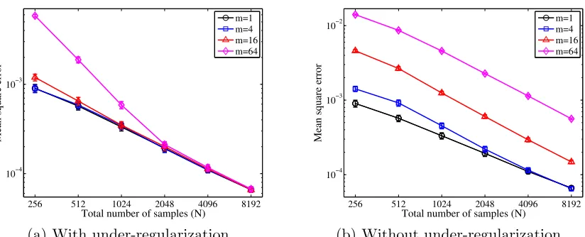
Figure 1: The squared L2(P)-norm between between the averaged estimate ¯f and the op-timal solution f∗. (a) These plots correspond to the output of the Fast-KRR algorithm: each sub-problem is under-regularized by using λ ' N−2/3. (b) Analogous plots when each sub-problem isnot under-regularized—that is, with λ=n−2/3 = (N/m)−2/3 chosen as if there were only a single dataset of sizen.
6.1 Simulation Studies
We begin by exploring the empirical performance of our subsample-and-average methods for a non-parametric regression problem on simulated datasets. For all experiments in this section, we simulate data from the regression model y = f∗(x) + ε for x ∈ [0,1], where f∗(x) := min(x,1−x) is 1-Lipschitz, the noise variables ε∼ N(0, σ2) are normally distributed with variance σ2 = 1/5, and the samples xi ∼ Uni[0,1]. The Sobolev space of Lipschitz functions on [0,1] has reproducing kernel K(x, x0) = 1 + min{x, x0} and norm
kfk2H=f2(0) +R01(f0(z))2dz. By construction, the function f∗(x) = min(x,1−x) satisfies kf∗kH= 1. The kernel ridge regression estimator fbtakes the form
b
f = N
X
i=1
αiK(xi,·), where α= (K+λN I)−1y, (37)
and K is the N ×N Gram matrix and I is the N ×N identity matrix. Since the first-order Sobolev kernel has eigenvalues (Gu, 2002) that scale as µj ' (1/j)2, the minimax convergence rate in terms of squaredL2(P)-error isN−2/3 (see e.g. Tsybakov (2009); Stone (1982); Caponnetto and De Vito (2007)).
By Corollary 4 withν = 1, this optimal rate of convergence can be achieved by Fast-KRR with regularization parameter λ ≈ N−2/3 as long as the number of partitions m satisfies m.N1/3. In each of our experiments, we begin with a dataset of sizeN =mn, which we partition uniformly at random intom disjoint subsets. We compute the local estimator fbi
for each of them subsets using n samples via (37), where the Gram matrix is constructed using the ith batch of samples (and n replaces N). We then compute ¯f = (1/m)Pm
0 0.2 0.4 0.6 0.8 1
10−5
10−4
10−3
10−2
10−1
log(# of partitions)/log(# of samples)
Mean square error
N=256 N=512 N=1024 N=2048 N=4096 N=8192
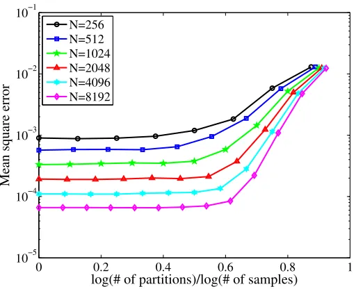
Figure 2: The mean-square error curves for fixed sample size but varied number of parti-tions. We are interested in the threshold of partitioning numberm under which the optimal rate of convergence is achieved.
Our experiments compare the error of ¯f as a function of sample size N, the number of partitions m, and the regularization λ.
In Figure 6.1(a), we plot the errorkf¯−f∗k2
2versus the total number of samplesN, where N ∈ {28,29, . . . ,213}, using four different data partitionsm∈ {1,4,16,64}. We execute each simulation 20 times to obtain standard errors for the plot. The black circled curve (m= 1) gives the baseline KRR error; if the number of partitionsm≤16, Fast-KRR has accuracy comparable to the baseline algorithm. Even withm= 64, Fast-KRR’s performance closely matches the full estimator for larger sample sizes (N ≥211). In the right plot Figure 6.1(b), we perform an identical experiment, but we over-regularize by choosing λ= n−2/3 rather thanλ=N−2/3 in each of themsub-problems, combining the local estimates by averaging as usual. In contrast to Figure 6.1(a), there is an obvious gap between the performance of the algorithms whenm= 1 and m >1, as our theory predicts.
It is also interesting to understand the number of partitions m into which a dataset of size N may be divided while maintaining good statistical performance. According to Corollary 4 with ν = 1, for the first-order Sobolev kernel, performance degradation should be limited as long as m.N1/3. In order to test this prediction, Figure 2 plots the mean-square errorkf¯−f∗k2
N m= 1 m= 16 m= 64 m= 256 m= 1024 212 Error 1.26·10
−4 1.33·10−4 1.38·10−4
N/A N/A
Time 1.12 (0.03) 0.03 (0.01) 0.02 (0.00)
213 Error 6.40·10
−5 6.29·10−5 6.72·10−5
N/A N/A
Time 5.47 (0.22) 0.12 (0.03) 0.04 (0.00)
214 Error 3.95·10
−5 4.06·10−5 4.03·10−5 3.89·10−5
N/A Time 30.16 (0.87) 0.59 (0.11) 0.11 (0.00) 0.06 (0.00)
215 Error Fail 2.90·10
−5 2.84·10−5 2.78·10−5
N/A Time 2.65 (0.04) 0.43 (0.02) 0.15 (0.01)
216 Error Fail 1.75·10
−5 1.73·10−5 1.71·10−5 1.67·10−5 Time 16.65 (0.30) 2.21 (0.06) 0.41 (0.01) 0.23 (0.01)
217 Error Fail 1.19·10
−5 1.21·10−5 1.25·10−5 1.24·10−5 Time 90.80 (3.71) 10.87 (0.19) 1.88 (0.08) 0.60 (0.02)
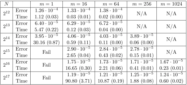
Table 1: Timing experiment giving kf¯−f∗k2
2 as a function of number of partitions m and data sizeN, providing mean run-time (measured in second) for each numbermof partitions and data size N.
Our final experiment gives evidence for the improved time complexity partitioning pro-vides. Here we compare the amount of time required to solve the KRR problem using the naive matrix inversion (37) for different partition sizesmand provide the resulting squared errorskf¯−f∗k2
2. Although there are more sophisticated solution strategies, we believe this is a reasonable proxy to exhibit Fast-KRR’s potential. In Table 1, we present the results of this simulation, which we performed in Matlab using a Windows machine with 16GB of memory and a single-threaded 3.4Ghz processor. In each entry of the table, we give the mean error of Fast-KRR and the mean amount of time it took to run (with standard deviation over 10 simulations in parentheses; the error rate standard deviations are an order of magnitude smaller than the errors, so we do not report them). The entries “Fail” corre-spond to out-of-memory failures because of the large matrix inversion, while entries “N/A” indicate thatkf¯−f∗k2 was significantly larger than the optimal value (rendering time im-provements meaningless). The table shows that without sacrificing accuracy, decomposition via Fast-KRR can yield substantial computational improvements.
6.2 Real Data Experiments
0 200 400 600 800 1000 80
80.5 81 81.5 82 82.5 83
Training runtime (sec)
Mean square error
Fast−KRR Nystrom Sampling Random Feature Approx.
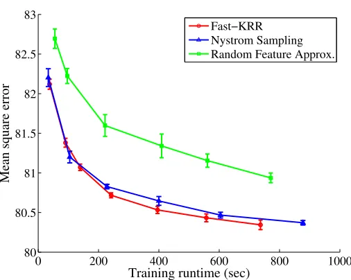
Figure 3: Results on year prediction on held-out test songs for Fast-KRR, Nystr¨om sam-pling, and random feature approximation. Error bars indicate standard deviations over ten experiments.
Our experiments with this dataset use the Gaussian radial basis kernel
K(x, x0) = exp −kx−x
0k2 2 2σ2
!
. (38)
We normalize the feature vectors x so that the timbre signals have standard deviation 1, and select the bandwidth parameter σ = 6 via cross-validation. For regularization, we set λ = N−1; since the Gaussian kernel has exponentially decaying eigenvalues (for typical distributions onX), Corollary 5 shows that this regularization achieves the optimal rate of convergence for the Hilbert space.
In Figure 3, we compare the time-accuracy curve of Fast-KRR with two approximation-based methods, plotting the mean-squared error between the predicted release year and the actual year on test songs. The first baseline is Nystr¨om subsampling (Williams and Seeger, 2001), where the kernel matrix is approximated by a low-rank matrix of rank r ∈ {1, . . . ,6} ×103. The second baseline approach is an approximate form of kernel ridge regression using random features (Rahimi and Recht, 2007). The algorithm approximates the Gaussian kernel (38) by the inner product of two random feature vectors of dimensions D ∈ {2,3,5,7,8.5,10} ×103, and then solves the resulting linear regression problem. For the Fast-KRR algorithm, we use seven partitions m ∈ {32,38,48,64,96,128,256} to test the algorithm. Each algorithm is executed 10 times to obtain standard deviations (plotted as error-bars in Figure 3).
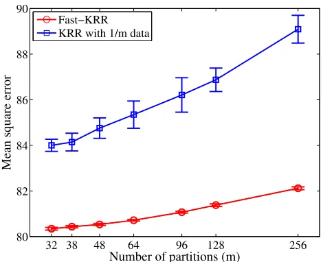
32 38 48 64 96 128 256 80
82 84 86 88 90
Number of partitions (m)
Mean square error
Fast−KRR KRR with 1/m data
Figure 4: Comparison of the performance of Fast-KRR to a standard KRR estimator using a fraction 1/mof the data.
algorithm, it is worth noting that with parallel computation, it is trivial to accelerate Fast-KRRmtimes; parallelizing approximation-based methods appears to be a non-trivial task. Moreover, as our results in Section 3 indicate, Fast-KRR is minimax optimal in many regimes. At the same time the conference version of this paper was submitted, Bach (2013) published the first results we know of establishing convergence results in`2-error for Nystr¨om sampling; see the discussion for more detail. We note in passing that standard linear regression with the original 90 features, while quite fast with runtime on the order of 1 second (ignoring data loading), has mean-squared-error 90.44, which is significantly worse than the kernel-based methods.
Our final experiment provides a sanity check: is the final averaging step in Fast-KRR even necessary? To this end, we compare Fast-KRR with standard KRR using a fraction 1/m of the data. For the latter approach, we employ the standard regularization λ ≈ (N/m)−1. As Figure 4 shows, Fast-KRR achieves much lower error rates than KRR using only a fraction of the data. Moreover, averaging stabilizes the estimators: the standard deviations of the performance of Fast-KRR are negligible compared to those for standard KRR.
7. Discussion
m.N/γ(λ)2, our method achieves estimation error decreasing as
Ekf¯−f∗k22
.λkf∗k2H+ σ 2γ(λ)
N .
(In particular, recall the bound (8) following Theorem 1). Notably, this convergence rate is minimax optimal, and we achieve substantial computational benefits from the subsampling schemes, in that computational cost scales (nearly) linearly inN.
It is also interesting to consider the number of kernel evaluations required to imple-ment our method. Our estimator requiresm sub-matrices of the full kernel (Gram) matrix, each of size N/m×N/m. Since the method may usem N/γ2(λ) machines, in the best case, it requires at most N γ2(λ) kernel evaluations. By contrast, Bach (2013) shows that Nystr¨om-based subsampling can be used to form an estimator within a constant factor of optimal as long as the number ofN-dimensional subsampled columns of the kernel matrix scales roughly as the marginal dimension eγ(λ) = Ndiag(K(K+λN I)−1)
∞.
Conse-quently, using roughlyNeγ(λ) kernel evaluations, Nystr¨om subsampling can achieve optimal
convergence rates. These two scalings–namely, N γ2(λ) versus Neγ(λ)—are currently not comparable: in some situations, such as when the data is not compactly supported, eγ(λ) can scale linearly with N, while in others it appears to scale roughly as the true effective dimensionality γ(λ). A natural question arising from these lines of work is to understand the true optimal scaling for these different estimators: is one fundamentally better than the other? Are there natural computational tradeoffs that can be leveraged at large scale? As datasets grow substantially larger and more complex, these questions should become even more important, and we hope to continue to study them.
Acknowledgments
We thank Francis Bach for interesting and enlightening conversations on the connections between this work and his paper (Bach, 2013) and Yining Wang for pointing out a mistake in an earlier version of this manuscript. We also thank two reviewers for useful feedback and comments. JCD was partially supported by a National Defense Science and Engineering Graduate Fellowship (NDSEG) and a Facebook PhD fellowship. This work was partially supported by ONR MURI grant N00014-11-1-0688 to MJW.
Appendix A. Proof of Lemma 6
This appendix is devoted to the bias bound stated in Lemma 6. LetX ={xi}ni=1 be short-hand for the design matrix, and define the error vector ∆ =fb−f∗. By Jensen’s
inequal-ity, we have kE[∆]k2 ≤ E[kE[∆|X]k2], so it suffices to provide a bound on kE[∆|X]k2. Throughout this proof and the remainder of the paper, we represent the kernel evaluator by the functionξx, whereξx:=K(x,·) andf(x) =hξx, fi for anyf ∈ H. Using this notation, the estimate fbminimizes the empirical objective
1 n
n
X
i=1
hξxi, fiH−yi
2
b
f Empirical KRR minimizer based on n samples
f∗ Optimal function generating data, where yi =f∗(xi) +εi ∆ Errorfb−f∗
ξx RKHS evaluatorξx:=K(x,·), sohf, ξxi=hξx, fi=f(x)
b
Σ Operator mappingH → Hdefined as the outer productΣ :=b 1n Pn
i=1ξxi⊗ξxi,
so that Σfb = n1 Pn
i=1hξxi, fiξxi
φj jth orthonormal basis vector forL2(P)
δj Basis coefficients of ∆ orE[∆|X] (depending on context), i.e. ∆ =P∞j=1δjφj θj Basis coefficients of f∗, i.e. f∗=P∞j=1θjφj
d Integer-valued truncation point
M Diagonal matrix with M = diag(µ1, . . . , µd) Q Diagonal matrix with Q= (Id×d+λM−1)
1 2
Φ n×dmatrix with coordinates Φij =φj(xi) v↓ Truncation of vector v. Forv=P
jνjφj ∈ H, defined asv
↓ =Pd
j=1νjφj; for v ∈`2(N) defined asv↓ = (v1, . . . , vd)
v↑ Untruncated part of vector v, defined asv↑= (vd+1, vd+1, . . .) βd The tail sum Pj>dµj
γ(λ) The sum P∞j=11/(1 +λ/µj) b(n, d, k) The maximum max{p
max{k,log(d)},max{k,log(d)}/n1/2−1/k} Table 2: Notation used in proofs
This objective is Fr´echet differentiable, and as a consequence, the necessary and sufficient conditions for optimality (Luenberger, 1969) offbare that
1 n
n
X
i=1
ξxi(hξxi,fb−f ∗i
H−εi) +λfb=
1 n
n
X
i=1
ξxi(hξxi,fbiH−yi) +λfb= 0, (40)
where the last equation uses the fact thatyi =hξxi, f ∗i
H+εi. Taking conditional expecta-tions over the noise variables{εi}ni=1 with the design X={xi}ni=1 fixed, we find that
1 n
n
X
i=1
ξxihξxi,E[∆|X]i+λE[fb|X] = 0.
Define the sample covariance operatorΣ :=b 1n Pn
i=1ξxi⊗ξxi. Adding and subtracting λf ∗
from the above equation yields
(Σ +b λI)E[∆|X] =−λf∗. (41)
Consequently, we see we havekE[∆|X]kH ≤ kf∗kH, sinceΣb 0.
basis{φj}∞
j=1:
E[∆|X] =
∞ X
j=1
δjφj, withδj =hE[∆|X], φjiL2(
P). (42)
For a fixed d ∈ N, define the vectors δ↓ := (δ1, . . . , δd) and δ↑ := (δd+1, δd+2, . . .) (we suppress dependence on dfor convenience). By the orthonormality of the collection {φj}, we have
kE[∆|X]k22 =kδk 2 2=kδ
↓k2 2+kδ
↑k2
2. (43)
We control each of the elements of the sum (43) in turn.
Control of the term kδ↑k2
2: By definition, we have kδ↑k22 = µd+1
µd+1
∞ X
j=d+1
δj2 ≤ µd+1
∞ X
j=d+1 δ2j µj
(i)
≤ µd+1kE[∆|X]k2H (ii)≤µd+1kf∗k2H, (44)
where inequality (i) follows sincekE[∆|X]k2H = P∞
j=1 δ2
j
µj; and inequality (ii) follows from
the bound kE[∆|X]kH≤ kf∗kH, which is a consequence of equality (41).
Control of the term kδ↓k2
2: Let (θ1, θ2, . . .) be the coefficients of f∗ in the basis {φj}. In addition, define the matrices Φ∈Rn×d by
Φij =φj(xi) fori∈ {1, . . . , n}, and j∈ {1, . . . , d}
and M = diag(µ1, . . . , µd)0∈Rd×d. Lastly, define the tail error vector v∈Rn by vi: =
X
j>d
δjφj(xi) =E[∆↑(xi)|X].
Letl∈Nbe arbitrary. Computing the (Hilbert) inner product of the terms in equation (41) withφl, we obtain
−λθl µl
=hφl,−λf∗i=Dφl,(Σ +b λ)E[∆|X] E
= 1 n
n
X
i=1
hφl, ξxii hξxi,E[∆|X]i+λhφl,E[∆|X]i=
1 n
n
X
i=1
φl(xi)E[∆(xi)|X] +λ δl µl .
We can rewrite the final sum above using the fact that ∆ = ∆↓+ ∆↑, which implies
1 n
n
X
i=1
φl(xi)E[∆(xi)|X] = 1 n
n
X
i=1 φl(xi)
d
X
j=1
φj(xi)δj +
X
j>d
φj(xi)δj
Applying this equality forl= 1,2, . . . , dyields
1 nΦ
TΦ +λM−1
δ↓=−λM−1θ↓− 1 nΦ
We now show how the expression (45) gives us the desired bound in the lemma. By defining the shorthand matrix Q= (I+λM−1)1/2, we have
1 nΦ
TΦ +λM−1 =I+λM−1+ 1 nΦ
TΦ−I =Q
I+Q−1
1 nΦ
TΦ−I
Q−1
Q. As a consequence, we can rewrite expression (45) to
I +Q−1
1 nΦ
TΦ−I
Q−1
Qδ↓ =−λQ−1M−1θ↓− 1 nQ
−1ΦTv. (46)
We now present a lemma bounding the terms in equality (46) to control δ↓. Lemma 10 The following bounds hold:
λQ
−1M−1θ↓
2
2≤λkf
∗k2
H, and (47a)
E
"
1 nQ
−1ΦTv
2 2
#
≤ ρ 4kf∗k2
Htr(K)βd
λ . (47b)
Define the event E :=
Q−1 n1ΦTΦ−I
Q−1
≤1/2 . Under Assumption A with
mo-ment bound E[φj(X)2k]≤ρ2k, there exists a universal constant C such that
P(Ec)≤
max
p
k∨log(d),k∨log(d) n1/2−1/k
Cρ2γ(λ) √
n
k
. (48)
We defer the proof of this lemma to Appendix A.1.
Based on this lemma, we can now complete the proof. Whenever the event E holds, we know thatI+Q−1((1/n)ΦTΦ−I)Q−1 (1/2)I. In particular, we have
kQδ↓k22 ≤4
λQ
−1M−1θ↓+ (1/n)Q−1ΦTv
2 2 on E, by Eq. (46). SincekQδ↓k2
2 ≥ kδ↓k22, the above inequality implies that kδ↓k22 ≤4
λQ
−1M−1θ↓+ (1/n)Q−1ΦTv
2 2 Since E isX-measurable, we thus obtain
E
h
kδ↓k22i=E
h
1(E)kδ↓k22i+E
h
1(Ec)kδ↓k22i ≤4E
1(E)
λQ
−1M−1θ↓
+ (1/n)Q−1ΦTv
2 2
+E
h
1(Ec)kδ↓k22i.
Applying the bounds (47a) and (47b), along with the elementary inequality (a+b)2 ≤ 2a2+ 2b2, we have
E
h
kδ↓k22i≤8λkf∗k2H+8ρ 4kf∗k2
Htr(K)βd λ +E
h
Now we use the fact that by the gradient optimality condition (41),
kE[∆|X]k22≤µ0kE[∆|X]k2H≤µ0kf∗k2H
Recalling the shorthand (6) forb(n, d, k), we apply the bound (48) to see
E
h
1(Ec)kδ↓k2 2
i
≤P(Ec)µ
0kf∗k2H≤
Cb(n, d, k)ρ2γ(λ) √
n
k
µ0kf∗k2H
Combining this with the inequality (49), we obtain the desired statement of Lemma 6.
A.1 Proof of Lemma 10
Proof of bound (47a): Beginning with the proof of the bound (47a), we have
Q
−1M−1θ↓
2 2 = (θ
↓
)T(M2+λM)−1θ↓ ≤(θ↓)T(λM)−1θ↓ = 1
λ(θ
↓
)TM−1θ↓≤ 1 λkf
∗k2
H.
Multiplying both sides by λ2 gives the result.
Proof of bound (47b): Next we turn to the proof of the bound (47b). We begin by re-writing Q−1ΦTv as the product of two components:
1 nQ
−1ΦTv= (M +λI)−1/2
1 nM
1/2ΦTv
. (50) The first matrix is a diagonal matrix whose operator norm is bounded:
(M+λI) −1/2
= max
j∈[d] 1
p
µj +λ ≤ √1
λ. (51) For the second factor in the product (50), the analysis is a little more complicated. Let Φ`= (φl(x1), . . . , φl(xn)) be the`th column of Φ. In this case,
M
1/2ΦTv
2 2 =
d
X
`=1
µ`(ΦT`v)2 ≤ d
X
`=1
µ`kΦ`k22kvk 2
2, (52)
using the Cauchy-Schwarz inequality. Taking expectations with respect to the design{xi}ni=1 and applying H¨older’s inequality yields
E[kΦ`k22kvk 2 2]≤
q
E[kΦ`k42]
q
E[kvk42].
We bound each of the terms in this product in turn. For the first, we have
E[kΦ`k42] =E
n
X
i=1
φ2`(Xi)
2
=E
n
X
i,j=1
φ2`(Xi)φ2`(Xj)