Training Highly Multiclass Classifiers
Maya R. Gupta [email protected]
Samy Bengio [email protected]
Google Inc.
1600 Amphitheatre Pkwy
Mountain View, CA 94301, USA
Jason Weston [email protected]
Google Inc. 76 9th Avenue,
New York, NY 10011 USA
Editor:Koby Crammer
Abstract
Classification problems with thousands or more classes often have a large range of class-confusabilities, and we show that the more-confusable classes add more noise to the em-pirical loss that is minimized during training. We propose an online solution that reduces the effect of highly confusable classes in training the classifier parameters, and focuses the training on pairs of classes that are easier to differentiate at any given time in the training. We also show that the adagrad method, recently proposed for automatically decreasing step sizes for convex stochastic gradient descent, can also be profitably applied to the non-convex joint training of supervised dimensionality reduction and linear classifiers as done in Wsabie. Experiments on ImageNet benchmark data sets and proprietary image recogni-tion problems with 15,000 to 97,000 classes show substantial gains in classificarecogni-tion accuracy compared to one-vs-all linear SVMs and Wsabie.
Keywords: large-scale, classification, multiclass, online learning, stochastic gradient
1. Introduction
Problems with many classes abound: from classifying a description of a flower as one of the over 300,000 known flowering plants (Paton et al., 2008), to classifying a whistled tune as one of the over 30 million recorded songs (Eck, 2013). Many practical multiclass problems are labelling images, for example face recognition, or tagging locations in vacation photos. In practice, the more classes considered, the greater the chance that some classes will be easy to separate, but that some classes will be highly confusable.
a form ofcurriculum learning, that is, of learning to distinguish easy classes before focusing on learning to distinguish hard classes (Bengio et al., 2009).
In this paper, we focus on classifiers that use a linear discriminant or a single prototypical feature vector to represent each class. Linear classifiers are a popular approach to highly multiclass problems because they are efficient in terms of memory and inference and can provide good performance (Perronnin et al., 2012; Lin et al., 2011; Sanchez and Perronnin, 2011). Class prototypes offer similar memory/efficiency advantages. The last layer of a deep belief network classifier is often linear or soft-max discriminant functions (Bengio, 2009), and the proposed ideas for adapting online loss functions should be applicable in that context as well.
We apply the proposed loss function adaptation to the multiclass linear classifier called Wsabie (Weston et al., 2011). We also simplify Wsabie’s weighting of stochastic gradients, and employ a recent advance in automatic step-size adaptation calledadagrad (Duchi et al., 2011). The resulting proposed Wsabie++classifier almost doubles the classification accuracy on benchmark Imagenet data sets compared to Wsabie, and shows substantial gains over one-vs-all SVMs.
The rest of the article is as follows. After establishing notation in Section 2, we explain in Section 3 how different class confusabilities can distort the standard empirical loss. We then review loss functions for jointly training multiclass linear classifiers in Section 4, and stochastic gradient descent variants for large-scale learning in Section 5. In Section 6, we propose a practical online solution to adapt the empirical loss to account for the variance of class confusability. We describe our adagrad implementation in Section 7. Experiments are reported on benchmark and proprietary image classification data sets with 15,000-97,000 classes in Section 8 and 9. We conclude with some notes about the key issues and unresolved questions.
2. Notation And Assumptions
We take as given a set of training data{(xt,Yt)}fort= 1, . . . , n, wherext∈Rdis a feature
vector andYt⊂ {1,2, . . . , G}is the subset of theGclass labels that are known to be correct labels for xt. For example, an image might be represented by set of features xt and have known labelsYt={dolphin,ocean,Half Moon Bay}. We assume a discriminant function
f(x;βg) has been chosen with class-specific parametersβg for each class withg= 1, . . . , G. The class discriminant functions are used to classify a test samplex as the class label that solves
arg max
g f(x;βg). (1)
Most of this paper applies equally well to “learning to rank,” in which case the output might be a top-ranked or ranked-and-thresholded list of classes for a test samplex. For simplicity, we restrict our discussion and metrics to the classification paradigm given by (1).
Many of the ideas in this paper can be applied to any choice of discriminant function
f(x, βg), but in this paper we focus on efficiency in terms of test-time and memory, and so we focus on class discriminants that are parameterized by a d-dimensional vector per class. Two such functions are: the inner product f(x;βg) = βgTx, and the squared `2
Euclidean distance discriminants, respectively. For example, one-vs-all linear SVMs use a linear discriminant, where theβg are each trained to maximize the margin between samples from the gth class and all samples from all other classes. The nearest means classifier (Hastie et al., 2001) uses an Euclidean distance discriminant where each class prototype βg is set to be the mean of all the training samples labelled with classg. Both the linear and nearest-prototype functions produce linear decision boundaries between classes. And with either the linear or Euclidean discriminants, the classifier has a total of G×dparameters, and testing as per (1) scales asO(Gd).
To reduce memory and test time, and also as a regularizer, it may be useful for the clas-sifier to include a dimensionality reduction matrix (sometimes called an embedding matrix)
W ∈ Rm×d, and then use linear or Euclidean discriminants in the reduced dimensionality space, for examplef(x;W, βg) =βgTW x orf(x;W, βg) =−(βg−x)TW(βg−x).
3. The Problem with a Large Variance in Class Confusability
The underlying goal when discriminatively training a classifier is to minimize expected classification error, but this goal is often approximated by the empirical classification errors on a given data set. In this section, we show that the expected error does not count errors between confusable classes (likedolphin andporpoise) the same as errors between separable classes (like cat and dolphin), whereas the empirical error counts all errors equally. Consequently, more confusable classes add more noise to the standard empirical error approximation of the expected error, and this confusable-class noise can adversely affect training.
Then in Section 6, we propose addressing this issue by changing the way we measure empirical loss to reduce the impact of errors between more-confusable classes.
3.1 Expected Classification Error Depends on Class Confusability
Define a classifier c as a map from an input feature vectorx to a class such that c:Rd →
1,2, . . . , G. Let I be the indicator function, and assume there exists a joint probability distributionPX,Y on the random feature vector X ∈Rd and classY ∈ {1,2, . . . , G}. Then
the expected classification error of classifierc is:
EX,Y[IY6=c(X)] =EX
EY|X[IY6=c(X)]
(2)
=EX
PY|X(Y 6=c(X))
because I is a Bernoulli random variable (3)
≈ 1
n
n X
t=1
PY|xt(Y 6=c(xt)),law of large numbers approximation (4)
≈ 1
n
n X
t=1
Iyt6=c(xt), (5)
Equations (3) and (4) show that the expected error depends on the probability that a given feature vector xt has corresponding random class label Yt equal to the classifier’s decision c(xt). For example, suppose that sample xt is equally likely to be class 1 or class 2, but no other class. If the classifier labels xt as c(xt) = 1, one should add PY|xt(Y 6= (c(xt) = 1)) = 1/2 to the approximate error given by (4). On the other hand, suppose that for another sample xj, the probability of class 1 is.99 and the probability of class 3 is .01. Then if the classifier calls c(xj) = 1 we should add PY|xt(Y 6= (c(xt) = 1)) = .01 to the loss, whereas if the classifier calls c(xj) = 3 we should add PY|xt(Y 6= (c(xt) = 1)) = .99 to the loss. This relative weighting based on class confusions is in contrast to the standard empirical loss given in (5) that simply counts all errors equally.
One can interpret the standard empirical loss given in (5) as the maximum likeli-hood approximation to (2) that estimates PY|xt given the training sample pair (xt, yt) as
ˆ
PY|xt(yt) = 1 and ˆPY|xt(g) = 0 for all other classes g. This maximum likelihood estimate converges asymptotically to (4), but for a finite number of training samples may produce a poor approximation. For binary classifiers, the approximation (5) may be quite good. We argue that (5) is generally a worse approximation as the number of classes increases. The key issue is that while the one-or-zero error approximation in (5) asymptotically converges to
PY|xt, itconverges more slowly when classes aremore confusable, and thus more-confusable classes add more “noise” to the approximation than less-confusable classes, biasing the empirical loss to overfit the noise of the more confusable class confusions.
Let us characterize this difference in noise. For any feature vector x and classifiercthe true class labelY is a random variable, and thus the indicator IY6=c(xt) in (5) is a random
indicator with a binomial distribution with parameter p=PY|xt(Y 6=c(xt)). The variance of the random indicator IY6=c(xt) is p(1−p), and thus the more confusable the classes, the
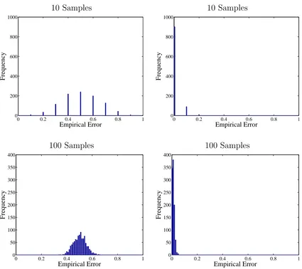
more variance there will be in the corresponding samples’ contribution to the empirical loss. Beyond noting the variance of the empirical errors is quadratic inp, it is not straightfor-ward to formally characterize the distribution of the empirical loss for binomials with differ-entpfor finiten(see for example Brown et al., 2001). However we can emphasize this point with a histogram of simulated empirical errors in Figure 1. The figure shows histograms of 1000 different simulations of the empirical error, calculated by averaging either 10 random samples (top) or 100 random samples (bottom) that either havep=PY|xt(Y 6=c(xt)) = 0.5 (left) orp=PY|xt(Y 6=c(xt)) = 0.01 (right).
The left-hand side of Figure 1 corresponds to samples x that are equally likely to be one of two classes, and so even the Bayes classifier is wrong half the time, such that p =
PY|xt(Y 6= c(xt)) = 0.5. The empirical error of such samples will eventually converge to the true error 0.5, but we see (top left) that the empirical error of ten such samples varies greatly! Even one hundred such samples (bottom left) are often a full .1 away from their converged value. This is in contrast to the right-hand examples corresponding to samples
xt that are easily classified such that p=PY|xt(Y 6=c(xt)) = 0.01. Their empirical error is generally much closer to the correct .01. Thus the more-confusable classes add more noise to the standard empirical loss approximation (5).
P
(classification error) =
.
5
P
(classification error) =
.
01
10 Samples 10 Samples
0 0.2 0.4 0.6 0.8 1
0 200 400 600 800 1000
Frequency
Empirical Error 0 0.2 0.4 0.6 0.8 1
0 200 400 600 800 1000
Frequency
Empirical Error
100 Samples 100 Samples
0 0.2 0.4 0.6 0.8 1
0 50 100 150 200 250 300 350 400
Frequency
Empirical Error 0 0.2 0.4 0.6 0.8 1
0 50 100 150 200 250 300 350 400
Frequency
Empirical Error
Empirical errors: 10 Empirical errors: 9
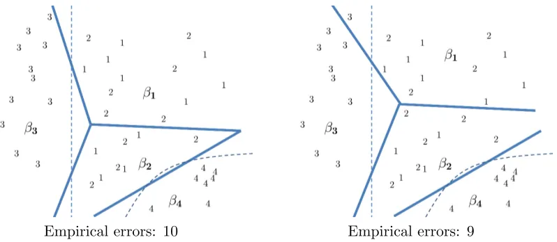
Figure 2: Two classifiers and the same draw of random training samples from four classes. Dotted lines correspond to the Bayes decision boundaries, and indicate that class 1 and class 2 are indistinguishable (same Bayes decision regions). Solid lines cor-respond to the classifier decision boundaries, determined by which class prototype
β1, β2, β3, or β4 is closest. The two figures differ in the placement of β1, which
produces different classifier decision boundaries. In this case, because of the ran-domness of the given training samples, the empirical error is higher for the left classifier than the right classifier, but the left classifier is closer to the optimal Bayes classifier.
Figure 2 shows an example of empirical error being overfit to noise between confusable classes. The figure compares two classifiers. Each classifier uses a Euclidean discriminant function, that is, the gth class is represented by a prototype vector {βg}, and a feature vector is classified as the nearest prototype with respect to Euclidean distance. Thus the decision boundaries are formed by the Voronoi diagram denoted with the thick lines, and the decision boundary between any two classes is linear.
The two classifiers in Figure 2 differ only in the placement ofβ1. One sees that decision
boundaries produced are not independent of each other: the right classifier has moved β1
up to reduce empirical errors between class 1 and class 2, but this also changes the decision boundary between classes 1 and 3, and incurs a new empirical error of a class 3 sample. The left classifier in Figure 2 is actually closer to the Bayes decision boundaries (shown by the dotted lines), and would have lower error on a test set (on average).
3.2 Two Factors We Mostly Ignore In This Discussion
Throughout this paper we ignore the dependence ofPY|x(Y 6=c(x)) on the particular feature vectorx, and focus instead on how confusable a particular classy =c(X) is averaged over
X. For example, pictures of porpoises may on average be confused with pictures of dolphins, even though a particular image of a porpoise may be more or less confusable.
Also, we have thus far ignored the fact that discriminative training usually makes a further approximation of (5) by replacing the indicator by a convex approximation like the hinge loss. Such convex relaxations do not avoid the issues described in the previous section, though they may help. For example, the hinge loss increases the weight of an error that is made farther from the decision boundary. To the extent that classes are less confusable farther away from the decision boundary, the hinge loss may be a better approximation than the indicator to the probabilistic weighting of (4). However, if the features are high-dimensional, the distribution of distances from the decision boundary may be less variable than one would expect from two-dimensional intuition (see for example Hall and Marron, 2005).
3.3 A Different Approximation for the Empirical Loss
We argued above that when computing the empirical test error, approximating PY|xt(Y 6=
c(xt)) by 1 if yt=c(xt) and by 0 otherwise adds preferentially more label noise from more confusable classes.
Here we propose a different approximation for PY|xt(Y 6=c(xt)). As usual, ifc(xt) =yt, we approximate PY|xt(Y 6= c(xt)) by 0. But if c(xt) 6= yt, then we use the empirical probability that a training sample that has labelyt is not classified asc(xt):
PY|xt(Y 6=c(xt))≈EX|Y=yt[P(c(X)6=c(xt)] (6)
≈
n X
τ=1
Iyτ=ytIc(xτ)6=c(xt) Pn
τ=1Iyτ=yt
Iyt6=c(xt). (7)
This approximation depends on how consistently feature vectors with training label yt are classified as classc(xt), and counts common class-confusions less. For example, consider the right-hand classifierc(x) in Figure 2. There is just one training sample labeled 3that is incorrectly classified as class1. The cost of that error according to (7) is 10/11, because there are eleven class 3 examples, and ten of those are classified as class 3. On the other hand, the cost of incorrectly labeling a sample of class 1 as a sample of class 2 would be only 7/11, because seven of the eleven class 1samples are not labeled as class 2.
Thus this approximation generally has the desired effect of counting confusions between confusable classes relatively less than confusions between easy-to-separate classes. This approximation is more exact for “good” classifiers c(x) that are more similar to the Bayes classifier, and more exact if the feature vectorsX are equally predictive for each class label so that averaging over X in (6) is a good approximation for most realizationsxt.
using the approximation (7) for the empirical loss. Shamir and Dekel (2010) proposed a related but more extreme two-step approach for highly multi-class problems: first train a classifier on all classes, and then delete classes that are poorly estimated by the classifier.
To be more practical, we propose continuously evolving the classifier to ignore the cur-rently highly-confusable classes by implementing (6) in an online fashion with SGD. This simple variant can be interpreted as implementing curriculum learning (Bengio et al., 2009), a topic we discuss further in Section 6.2.1. But before detailing the proposed simple on-line strategy in Section 6, we need to review related work in loss functions for multi-class classifiers.
4. Related Work in Loss Functions for Multiclass Classifiers
In this section, we review loss functions for multiclass classifiers, and discuss recent work adapting such loss functions to the online setting for large-scale learning.
One of the most popular classifiers for highly multiclass learning is one-vs-all linear SVMs, which have only O(Gd) parameters to learn and store, and O(Gd) time needed for testing. A clear advantage of one-vs-all is that the G class discriminant functions
{fg(x)} can be trained independently. An alternate parallelizable approach is to train all
G2 one-vs-one SVMs, and let them vote for the best class (also known as round-robin and all-vs-all). Binary classifiers can also be combined using error-correcting code approaches (Dietterich and Bakiri, 1995; Allwein et al., 2000; Crammer and Singer, 2002). A well-regarded experimental study of multiclass classification approaches by Rifkin and Klatau (2004) showed that one-vs-all SVMs performed “just as well” on a set of ten benchmark data sets with 4-49 classes as one-vs-one or error-correcting code approaches.
A number of researchers have independently extended the two-class SVM optimization problem to a joint multiclass optimization problem that maximizes pairwise margins subject to the training samples being correctly classified, with respect to pairwise slack variables (Vapnik, 1998; Weston and Watkins, 1998, 1999; Bredensteiner and Bennet, 1999).1 These extensions have been shown to be essentially equivalent quadratic programming problems (Guermeur, 2002). The minimized empirical loss can be stated as the sum of the pairwise errors:
Lpairwise({βg}) = n X
t=1
1
|Yt| X
y+∈Yt
1
|YC t |
X
y−∈YC t
|b−f(xt;βy+) +f(xt;βy−)|+, (8)
where| · |+ is short-hand for max(0,·),b is a margin parameter,YC
t is the complement set ofYt, and we added normalizers to account for the case that a givenxtmay have more than one positive label such that|Yt|>1.
Crammer and Singer (2001) instead suggested taking the maximum hinge loss over all the negative classes:
Lmax loss({βg}) = n X
t=1
1
|Yt| X
y+∈Y
t
max y−∈YC
t
|b−f(xt;βy+) +f(xt;βy−)|+. (9)
This maximum hinge-loss is sometimes called multiclass SVM, and can be derived from a margin-bound (Mohri et al., 2012). Daniely et al. (2012) theoretically compared multiclass SVM with one-vs-all, one-vs-one, tree-based linear classifiers and error-correcting output code linear classifiers. They showed that the hypothesis class of multiclass SVM contains that of all and tree-classifiers, which strictly contain the hypothesis class of one-vs-one classifiers. Thus the potential performance with multiclass SVM is larger. However they also showed that the approximation error of one-vs-one is smallest, with multiclass SVM next smallest.
Statnikov et al. (2005) compared eight multiclass classifiers including that of Weston and Watkins (1999) and Crammer and Singer (2001) on nine cancer classification problems with 3 to 26 classes and less than 400 samples per problem. On these small-scale data sets, they found the Crammer and Singer (2001) classifier was best (or tied) on 2/3 of the data sets, and the pairwise loss given in (8) performed almost as well.
Lee et al. (2004) prove in their Lemma 2 that previous approaches to multiclass SVMs are not guaranteed to be asymptotically consistent. For more on consistency of multiclass classification loss functions, see Rifkin and Klatau (2004), Tewari and Bartlett (2007), Zhang (2004), and Mroueh et al. (2012). Lee et al. (2004) proposed a multiclass loss function that is consistent. They force the class discriminants to sum to zero such that P
gf(x;βg) = 0 for all x, and define the loss:
Ltotal loss({βg}) = n X
t=1
X
y−∈YC t
|f(xt;βy−)− 1
G−1|+. (10)
This loss function jointly trains the class discriminants so that the total sum of wrong class discriminants for each training sample is small. Minimizing this loss can be expressed as a constrained quadratic program. The experiments of Lee et al. (2004) on a few small data sets did not show much difference between the performance of (10) and (8).
5. Online Loss Functions for Training Large-scale Multiclass Classifiers
If there are a large number of training samplesn, then computing the loss for each candidate set of classifier parameters becomes computationally prohibitive. The usual solution is to minimize the loss in an online fashion with stochastic gradient descent, but exactly how to sample the stochastic gradients becomes a key issue. Next, we review two stochastic gradient approaches that correspond to different loss functions: AUC sampling (Grangier and Bengio, 2008) and the WARP sampling used in the Wsabie classifier (Weston et al., 2011).
5.1 AUC Sampling
For a large number of training samplesn, Grangier and Bengio (2008) proposed optimizing (8) by sequentially uniformly sampling from each of the three sums in (8):
1. draw one training sample xt,
3. draw one incorrect classy− fromYC t ,
4. compute the corresponding stochastic gradient of the loss in (8),
5. update the classifier parameters.
This sampling strategy, referred to asarea under the curve(AUC)sampling, is inefficient because most randomly drawn incorrect class samples will have zero hinge loss and thus not produce an update to the classifier.
5.2 WARP Sampling
The weighted approximately ranked pairwise (WARP) sampling was introduced by Weston et al. (2011) to make the stochastic gradient sampling more efficient than AUC sampling, and was evolved from the weighted pairwise classification loss of Usunier et al. (2009). Unlike AUC sampling, WARP sampling focuses on sampling from negative classes that produce non-zero stochastic gradients for a given training example.
To explain WARP sampling, we first define the WARP loss:
LWARP({βg}) = n X
t=1
1
|Yt| X
y+∈Y
t 1
|Vt,y+|
X
yv∈V t,y+
w(y+) |b−f(xt;βy+) +f(xt;βyv)|+, (11)
wherew(y+) is a weight on the correct label, andVt,y+ is the set ofviolating classes defined:
Vt,y+ ={yv s.t. |b−f(xt;βy+) +f(xt;βyv)|+>0}. (12) As in Usunier et al. (2009), Weston et al. (2011) suggest using a weight function w(y+) that is an increasing function of the number of violating classes. Because the number of violating classes defines the rank of the correct class y+, they denote the number of violating classes for a training sample with training class y+ as r(y+). They suggest using the truncated harmonic series for the weight function,
w(y+) = r(y+)
X
j=1
1
j. (13)
Weston et al. (2011) proposed WARP sampling which sequentially uniformly samples from each of the three sums in (11):
1. draw one training sample xt,
2. draw one correct classy+ from Yt,
3. draw one violating classyv from Vt,y+ if one exists,
4. compute the corresponding stochastic gradient of the loss in (11),
To sample a violating class fromVt,y+, the negative classes inYtCare uniformly randomly
sampled until a class that satisfies the violation constraint (12) is found, or the number of allowed such trials (generally set to beG) is exhausted. The rankr(y+) needed to calculate the weight in (13) is estimated to be (G−1) divided by the number of negative classes
y−∈ Yt that had to be tried before finding a violating classyv from Vt,y+.
5.3 Some Notes Comparing AUC and WARP Loss
We note that WARP sampling is more likely than AUC sampling to update the parameters of a training sample’s positive class y+ if y+ has few violating classes, that is if (x
t, yt) is already highly-ranked by (1). Specifically, suppose a training pair (xt, yt) is randomly sampled, and suppose H > 0 of the G classes are violators such that their hinge-loss is non-zero with respect to (x, y+). WARP sampling will draw random classes until it finds
a violator and makes an update, but AUC will only make an update if the one random class it draws happens to be a violator, so only H/(G−1) of the time. By definition, the higher-ranked the correct class yt is for xt, the smaller the number of violating classes H, and the less likely AUC sampling will update the classifier to learn from (xt, yt).
In this sense, WARP sampling is more focused on fixing class parameters that are almost right already, whereas AUC sampling is more focused on improving class parameters that are very wrong. At test time, classifiers choose only the highest-ranked class discriminant as a class label, and thus the fact that AUC sampling updates more often on lower-ranked classes is likely the key reason that WARP sampling performs so much better in practice (see the experiments of Weston et al. (2011) and the experiments in this paper). Even in ranking, it is usually only the top ranked classes that are of interest. However, the WARP weight w(y+) given in (13) partly counteracts this difference by assigning greater weights (equivalently a larger step-size to the stochastic gradient) if the correct class has many violators, as then its rank is lower. In this paper, one of the proposals we make is to use constant weightsw(y+) = 1, so the training is even more focused on improving classes that are already highly-ranked.
AUC sampling is also inefficient because so many of the random samples result in a zero gradient. In fact, we note that the probability that AUC sampling will update the classifier
decreases if there are more classes. Specifically, suppose for a given training sample pair (xt, yt) there are H classes that violate it, and that there are G classes in total. Then the probability that AUC sampling updates the classifier for (xt, yt) isH/(G−1), which linearly decreases as the number of classes Gis increased.
5.4 Online Versions of Other Multiclass Losses
WARP sampling implements an online version of the pairwise loss given in (8) (Weston et al., 2011). One can also interpret the WARP loss sampling as an online approximation of the maximum hinge loss given in (9), where the maximum violating class is approximated by the sampled violating class. This interpretation does not call for a rank-based weighting
sampling multiple violating classes and then taking the class with the worst discriminant, we did not try this due to the expected time needed to find multiple violating classes. Further, we hypothesize that choosing the class with the largest violation as the violating class could actually perform poorly for practical highly multiclass problems like Imagenet because the worst discriminant may belong to a class that is a missing correct label, rather than an incorrect label.
An online version of the loss proposed by Lee et al. (2004) and given in (10) would be more challenging to implement because the G class discriminants are required to be normalized; we do not know of any such experiments.
5.5 The Wsabie Classifier
Weston et al. (2011) combined the WARP sampling with online learning of a supervised linear dimensionality reduction. They learn an embedding matrixW ∈Rm×d that maps a
given d-dimensional feature vector x to an m-dimensional “embedded” vector W x ∈ Rm, where m ≤ d, and then the G class-specific discriminants of dimension m are trained to separate classes in the embedding space. Weston et al. (2011) referred to this combination as the Wsabie classifier. This changes the WARP loss given in (11) to the non-convex Wsabie loss, defined:
LWsabie(W,{βg}) = n X
t=1
X
y+∈Y
t
X
yv∈V t,y+
w(y+) |b−f(W xt;βy+) +f(W xt;βyv)|+.
Adding the embedding matrixW changes the number of parameters fromGd toGm+
md. For a large number of classes G and a small embedding dimension m (the case of interest here) this reduces the overall parameters, and so the addition of the embedding matrixW acts as a regularizer, reduces memory, and reduces testing time.
6. Online Adaptation of the Empirical Loss to Reduce Impact of Highly Confusable Classes
In this section, we present a simple and memory-efficient online implementation of the empirical class-confusion loss we proposed in Section 3.3 that reduces the impact of highly confusable classes on the standard empirical loss. First, we describe the batch variant of this proposal and quantify its effect. Then in Section 6.2 we describe a sampling version. In Section 6.3, we propose a simple extension that experimentally increases the accuracy of the resulting classifier, without using additional memory. We show the proposed online strategy works well in practice in Section 9.
6.1 Reducing the Effect of Highly Confusable Classes By Ignoring Last Violators
We introduce the key idea of a last violator class with a simple example before a formal definition. Suppose during online training the hundredth training sample x100 has label
y100 = tiger, and that the last training sample we saw labelled tiger was x5. And
f(x5;θtiger) +f(x5;θlion)|+>0. Then for sample (x100,tiger) we call the class lion the last violator class.
Formally, we call class vt,y+ a last violator for the training sample pair (xt, y+) if xτ
was the last training sample for which y+ was the sampled positive class and vt,y+ was a
violator for (xτ, y+), that is, vt,y+ ∈ Vτ,y+. The set of violators Vτ,y+ becomes the set of
last violators of (xt, y+), which we denote ˜Vt,y+.
In order to decrease the effect of highly confusable classes on training the classifier, we propose to ignore losses for any violator class that was also a last violator class. The reasoning is that if the last violator class and a current violator class are the same, it indicates that the class yt and that violator class are consistently confused (for example
tiger and lion). And if two classes are consistently confused, we would like to reduce their impact on the empirical loss, as discussed in Section 3.
For example, say sequential training samples that were labelled cat had the following violating classes:
dogand pig, dogand pig, none, dog, dog, none, dog, pig.
The proposed approach ignores any violator that was also a last violator:
dogand pig,
dogandpig, none, dog, dog, none, dog, pig.
Mathematically, to ignore last violators we simply add an indicator function I to the
loss function. For example, ignoring last violators with the WARP loss from (11) can be written:
Lproposed({θg}) = n X
t=1
X
y+∈Y
t
X
yv∈V t,y+
w(y+) |b−f(xt;θy+) +f(xt;θyv)|+ I
yv6∈V˜t,y+.
(14)
That is, instead of forming one estimate of the correct empirical loss as we proposed in Section 3.3, here we approximate the correct empirical loss as the average of the series of Bernoulli random variables represented by the extra indicator in (14). In fact, the proposal to ignore last violators implements the proposed approximation (7): the probability that an error is not-counted is the probability that the violating class is confused with the training class:
Proposition 1: Suppose there are n samples labelled class g, and each such sample has probability pof being classified as class h. Then the expected number of losses summed in (11) isnp, but the expected number of losses summed in (14) is (n−1)p(1−p) +p.
6.2 Ignoring Sampled Last Violators for Online Learning
Building on the WARP sampling proposed by Weston et al. (2011) and reviewed in Section 5.2, we propose an online sampling implementation of (14), where for each classy+we store one sampled last violator and only update the classifier if the current violator is not the same as the last violator. Specifically,
1. draw one training sample xt,
2. draw one correct classy+ from Yt,
3. if there is no last violatorvt,y+ or ifvt,y+ exists but is not a violator for (xt, y+), then
draw and store one violating classyv from V y+ and
(a) compute the corresponding stochastic gradient of the loss in (8)
(b) update the parameters.
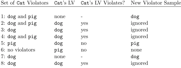
Table 1 re-visits the same example as earlier, and illustrates for eight sequential training examples whose training label was cat what the last violator class is, whether the last violator is a current violator (in which case the current error is ignored), or if not ignored, which of the current violators is randomly sampled for the classifier update.
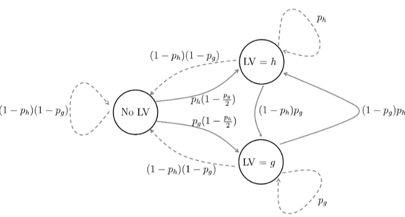
Throughout the training, the state of the sampled last violator for any class y+ can be viewed as a Markov chain. We illustrate this for the class y+ and two possible violating classesg and h in Figure 3.
In the experiments to follow, we couple the proposed online empirical class-confusion loss sampling strategy with an embedding matrix as in the Wsabie algorithm for efficiency and regularization, and refer to this as Wsabie++. A complete description of Wsabie++ is given in Table 3, including the adagrad stepsize updates described in the next section. The memory needed to implement this discounting isO(G) because only one last violator class is stored for each of theG classes.
Set of CatViolators Cat’s LV Cat’s LV Violates? New Violator Sampled?
1: dogand pig none - dog
2: dogand pig dog yes ignored
3: dog dog yes ignored
4: dogand pig dog yes ignored
5: pig dog no pig
6: no violators pig no none
7: dog none - dog
8: dog dog yes ignored
Figure 3: In the proposed sampling strategy for the online empirical class-confusion loss, the state of the last violator (LV) for a classy+ can be interpreted as a Markov chain where a transition occurs for each training sample. The figure illustrates the case where there are just two possible violating classes, classgand class h, which violate samples of classy+with probabilitypg andph respectively. Then the last violator for class y+ is always in one of three possible states: no last violator, class h is the last violator, or class g is the last violator. Solid lines indicate a violation that is counted; dotted lines indicate a violation that is ignored. The three states have stationary distribution:
P(No LV) = 1
Z,
P(LV =g) = 1
Z
pg(2 +ph−pgph) 2(pg−1)(pgph−1)
,
P(LV =h) = 1
Z
ph(2 +pg−pgph) 2(ph−1)(pgph−1)
,
True Class Last Violator Class
tiger → lion
lion → cat
cat → kitten
kitten → panther
panther → cat
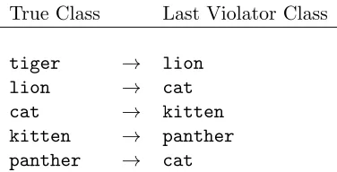
Table 2: Example chain of five classes and their sampled last violator.
6.2.1 Curriculum Learning
We have primarily motivated ignoring last violators as a better approximation for the ex-pected classification error. However, because this approach is online, it has a second practi-cal effect of changing the distribution of classifier updates as the classifier improves during training. Consider the classifier at some fixed point during training. At that point, classes that are better separated from all other classes are less likely to have a last violator stored, and thus more likely to be trained on. This increases the chance that the classifier first learns to separate easy-to-separate classes. At each point in time, the classifier is less likely to be updated to separate classes it finds most confusable. Bengio et al. (2009) have argued that this kind of easy-to-hard learning is natural and useful, particularly when optimizing non-convex loss functions as is the case when one jointly learns an embedding matrix W
for efficiency and regularization.
6.3 Extending the Discounting Loss to Multiple Last Violators
Table 2 shows an example of five classes and what their last violator class might be at some point in the online training. For example, Table 2 suggests that tigerand lion are highly confusable, and that lion and catare highly confusable, and thus we suspect that tiger and cat may also be highly confusable. To further reduce the impact of these sets of highly confusable classes, we extend the above approach to ignoring a training sample if it is currently violated by its last violator class’s last violator class, and so on. The longer the chain of last violators we choose to ignore, the more training samples are ignored, and the ignored training samples are preferentially those belonging to clusters of classes that are highly-confusable with each other.
Formally, let v2t,y+ denote the last violator of the last violator of y+, that is vt,y2 + = vt,vt,y+. For the example given in Table 2, ify
+ is tiger, then its last violator is v t,y+ =
lion, and v2
t,y+ =cat. More generally, let v
Q
t,y+ be theQth-order last violator, for example vt,3tiger=kitten.
Let ˜VQ
t,y+ be the set of last violators up through order Q for positive class y+ and the tth sample. We extend (14) to ignore this larger set of likely highly-confusable classes:
Lproposed-Q({θg}) = n X
t=1
X
y+∈Y
t
X
yv∈V t,y+
|b−f(xt;y+) +f(xt;yv)|+ Iyv6∈V˜Q t,y+
To use (15) in an online setting, each time a training sample and its positive class are drawn, we check if anyq-th order last violatorvqt,y+ for anyq ≤Qis a current violator, and
if so, we ignore that training sample and move directly to the next training sample without updating the classifier parameters.
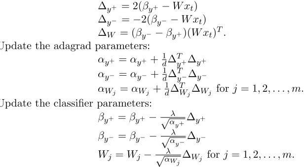
Table 3 gives the complete proposed sampling and updating algorithm for Euclidean discriminant functions, including the adaptive adagrad step-size explained in Section 7 which follows. For Euclidean discriminant functions we did not find (experimentally) that we needed any constraints or additional regularizers on W or {βg}, though if desired a regularization step can be added.
7. Adagrad For Learning Rate
Convergence speed of stochastic gradient methods is sensitive to the choice of stepsizes. Recently, Duchi et al. (2011) proposed a parameter-dependent learning rate for stochastic gradient methods. They proved that their approach has strong theoretical regret guarantees for convex objective functions, and experimentally it produced better results than compa-rable methods such as regularized dual averaging (Xiao, 2010) and the passive-aggressive method (Crammer et al., 2006). In our experiments, we applied adagrad both to the convex training of the one-vs-all SVMs and AUC sampling, as well as to the non-convex Wsabie++ training. Inspired by our preliminary results using adagrad for non-convex optimization, Dean et al. (2012) also tried adagrad for non-convex training of a deep belief network, and also found it produced substantial improvements in practice.
The main idea behind adagrad is that each parameter gets its own stepsize, and each time a parameter is updated its stepsize is decreased to be proportional to the running sum of the magnitude of all previous updates. For simplicity, we limit our description to the case where the parameters being optimized are unconstrained, which is how we implemented it. For memory and computational efficiency, Duchi et al. (2011) applying adagrad separately for each parameter (as opposed to modeling correlations between parameters).
We applied adagrad to adapt the stepsize for the G classifier discriminants {βg} and the m×dembedding matrix W. We found that we could save memory without affecting experimental performance by averaging the adagrad learning rate over the embedding di-mensions such that we keep track of one scalar adagrad weight per class. That is, let ∆g,τ denote the stochastic gradient for βg at timeτ, then we updateβg as follows:
βg,t+1=βg,t−η t X
τ=0
∆Tτ,g∆τ,g
d
!!−1/2
∆g,τ. (16)
Model:
Training Data Pairs: (xt,Yt) for t= 1,2, . . . , n
Embedded Euclidean Discriminant: f(W x;βg) =−(βg−W x)T(βg−W x)
Hyperparameters:
Embedding Dimension: m
Stepsize: λ∈R+
Margin: b∈R+
Depth of last violator chain: Q∈N
Initialize:
Wj,r set randomly to −1 or 1 forj= 1,2, . . . , m,r= 1,2, . . . , d
βg =0 for allg= 1,2, . . . , G
αg =0 for all g= 1,2, . . . , G
αWj =0for all j= 1,2, . . . , m
vy+ = empty set for ally+
While Not Converged:
Samplext uniformly from{x1, . . . , xn}. Sampley+ uniformly fromYt.
If |b−f(W xt;βy+) +f(W xt;βvq
y+)|+>0 for anyq = 1,2, . . . , Q,continue.
Set foundViolator = false. For count = 1 toG:
Sampley− uniformly fromYC t .
If |b−f(W xt;βy+) +f(W xt;βy−)|+>0, set foundViolator = true and break. If foundViolator = false, set vy+ to the empty set andcontinue.
Setvy+ =y−.
Compute the stochastic gradients:
∆y+ = 2(βy+−W xt)
∆y− =−2(βy−−W xt) ∆W = (βy−−βy+)(W xt)T.
Update the adagrad parameters:
αy+ =αy+ +1
d∆ T y+∆y+ αy− =αy−+1
d∆ T y−∆y−
αWj =αWj +1d∆WjT ∆Wj forj= 1,2, . . . , m. Update the classifier parameters:
βy+ =βy+−√λ
αy+∆y+ βy− =βy−−√λ
αy−∆y−
Wj =Wj −√αλ
Wj∆Wj forj= 1,2, . . . , m.
predominant, which we tested by setting the learning rate for each parameter proportional to the inverse square root of the number of times that parameter has been updated. This “counting adagrad” produced results that were not statistically different using (16). (The experimental results in this paper are reported using adagrad proper as per (16).)
We useα to refer to the running sum of gradient magnitudes in the complete Wsabie++ algorithm description given in Table 3.
8. Experiments
We first detail the data sets used. Then in Section 8.2 we describe the features. In Section 8.3 we describe the different classifiers compared and how the parameters and hyperparameters were set.
8.1 Data Sets
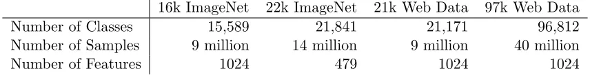
Experiments were run with four data sets, as summarized in Table 4 and detailed below.
16k ImageNet 22k ImageNet 21k Web Data 97k Web Data
Number of Classes 15,589 21,841 21,171 96,812
Number of Samples 9 million 14 million 9 million 40 million
Number of Features 1024 479 1024 1024
Table 4: Data sets.
8.1.1 ImageNet Data Sets
ImageNet (Deng et al., 2009) is a large image data set organized according to WordNet (Fellbaum, 1998). Concepts in WordNet, described by multiple words or word phrases, are hierarchically organized. ImageNet is a growing image data set that attaches one of these concepts to each image using a quality-controlled human-verified labeling process.
We used the spring 2010 and fall 2011 releases of the Imagenet data set. The spring 2010 version has around 9M images and 15,589 classes (16k ImageNet). The fall 2011 version has about 14M images and 21,841 classes (22k ImageNet). For both data sets, we separated out 10% of the examples for validation, 10% for test, and the remaining 80% was used for training.
8.1.2 Web Data Sets
We also had access to a large proprietary set of images taken from the web, together with a noisy annotation based on anonymized users’ click information. We created two data sets from this corpus that we refer to as 21k Web Data and 97k Web Data. The 21k Web Data contains about 9M images, divided into 20% for validation, 20% for test, and 60% for train, and the images are labelled with 21,171 distinct classes. The 97k Web Data contains about 40M images, divided into 10% for validation, 10% for test, and 80% for train, and the images are labelled with 96,812 distinct classes.
In contrast, the Web Data labels are taken from a set of popular queries that were the input to a general-purpose image search engine, so it includes people, brands, products, and abstract concepts. Second, the number of images per label in Imagenet is artificially forced to be somewhat uniform, while the Web Data distribution of number of images per label is generated by popularity with users, and is thus more exponentially distributed. Third, because of the popular origins of the Web data sets, classes may be translations of each other, plural vs. singular concepts, or synonyms (for examples, see Table 7). Thus we expect more highly-confusable classes for the Web Data than ImageNet. A fourth key difference is Imagenet disambiguates polysemous labels whereas Web Data does not, for example, an image labeled palm might look like the palm of a hand or like a palm tree. The fifth difference is that there may be multiple given positive labels for some of the Web samples, for example, the same image might be labelled mountain,mountains, Himalaya, and India.
Lastly, classes may be at different and overlapping precision levels, for example the class cake and the classwedding cake.
8.2 Features
We do not focus on feature extraction in this work, although features certainly can have a big impact on performance. For example, Sanchez and Perronnin (2011) recently achieved a 160% gain in accuracy on the 10k ImageNet datatset by changing the features but not the classification method.
In this paper we use features, similar to those used in Weston et al. (2011). We first combined multiple spatial (Grauman and Darrell, 2007) and multiscale color and texton histograms (Leung and Malik, 1999) for a total of about 5×10⁵dimensions. The descriptors are somewhat sparse, with about 50000 non-zero weights per image. Some of the constituent histograms are normalized and some are not. We then perform kernel PCA (Schoelkopf et al., 1999) on the combined feature representation using the intersection kernel (Barla et al., 2003) to produce a 1024-dimensional or 479-dimensional input vector per image (see Tab. 4), which is then used as the feature vectors for the classifiers.
8.3 Classifiers Compared and Hyperparameters
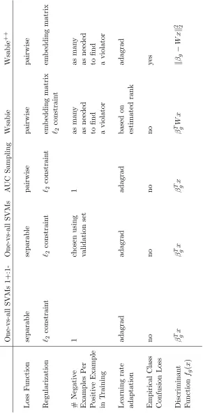
We experimentally compared the following linear classifiers: nearest means, one-vs-all SVMs, AUC, Wsabie, and the proposed Wsabie++ classifiers. Table 5 compares these methods as they were implemented for the experiments.
The nearest means classifier is the most efficient to train of the compared methods as it only passes over the training samples once and computes the mean of the training feature vectors for each class (and there are no hyperparameters).
One-vs-all SVMs 1+:1-On e -vs-all SVMs A UC Sampling Wsabie Wsabie ++ Loss F unction separable separ able pairwise pairwise pairwise Regularization `2 constrain t `2 constrain t `2 constrain t em b edding matrix em b edding matrix `2 constrain t # Negativ e 1 chosen using 1 as man y as man y Examples P er v alidation set as needed as needed P ositiv e Example to find to find in T raining a violator a violator Learning rate adagrad adagrad adagrad based on adagrad adaptation estimated rank Empirical Class no no no no y es Confusion Loss Discriminan t β
T gx
β
T gx
β
T gx
β
T gW
One-vs-all linear SVMs are the most popular choice for large-scale classifiers due to stud-ies showing their good performance, their parallelizable training, relatively small memory, and fast test-time (Rifkin and Klatau, 2004; Deng et al., 2010; Sanchez and Perronnin, 2011; Perronnin et al., 2012; Lin et al., 2011). Perronnin et al. (2012) highlights the importance of getting the right balance of negative to positive examples used to train the one-vs-all linear SVMs. As in their paper, we cross-validate the expected number of negative ex-amples per positive example; the allowable choices were powers of 2. In contrast, earlier published results by Weston et al. (2011) that compared Wsabie to one-vs-all SVMs used one negative example per positive example, analogous to the AUC classifier. We included this comparison, which we labelled One-vs-all SVMs 1+:1- in the tables.
Both Wsabie and Wsabie++jointly train an embedding matrixW as described in Section 3.5. The embedding dimension d was chosen on the validation set from the choices d =
{32,64,96,128,192,256,384,512,768,1024}embedding dimensions. In addition, we created
ensembleWsabie and Wsabie++classifiers by concatenatingbmdcsuchd-dimensional models to produce a classifier with a total ofm parameters to compare classifiers that require the same memory and test-time.
All hyperparameters were chosen based on the accuracy on a held-out validation set. Step-size, margin, and regularization constant hyperparameters were varied by powers of ten. The orderQ of the last violators was varied by powers of 2. Chosen hyperparameters are recorded in Table 9. Both the pairwise loss and Wsabie classifier are implemented with standard`2 constraints on the class discriminants (and for Wsabie, on the rows of the
embedding matrix). We did not use any regularization constraints for Wsabie++.
We initialized the Wsabie parameters and SVM parameters uniformly randomly within the constraint set. We initialize the proposed training by setting allβg to the origin, and all components of the embedding matrix are equally likely to be−1 or 1. Experiments with dif-ferent initialization schemes for these difdif-ferent classifiers showed that difdif-ferent (reasonable) initializations gave very similar results.
With the exception of nearest means, all classifiers were trained online with stochastic gradients. We also used adagrad for the convex optimizations of both one-vs-all SVMs and the AUC sampling, which increased the speed of convergence.
Recently, Perronnin et al. (2012) showed good results with one-vs-all SVM classifiers and the WARP loss where they also cross-validated an early-stopping criterion. Adagrad reduces step sizes over time, and this removed the need to worry about early stopping. In fact, we did not see any obvious overfitting with any of the classifier training (validation set and test set errors were statistically similar). Each algorithm was allowed to train on up to 100 loops through the entire training set or until the validation set performance had not changed in 24 hours. Even those runs that ran the entire 100 loops appeared to have essentially converged. Implemented in C++ without parallelization, all algorithms (except nearest means) took around one week to train the 16k Imagenet data set, around two weeks to train the 21k and 22k data sets, and around one month to train the 97k data set. Also in all cases roughly 80% of the validation accuracy was achieved in roughly the first 20% of the training time.
and parameters for the run that had the best accuracy on the validation set. For one-vs-all SVMs with its convex objective, the five runs usually differed by .1% (absolute), whereas optimizing the nonconvex objectives of Wsabie and Wsabie++produced much greater ran-domness within five runs, as much as .5% (absolute). Cross-validating substantially more runs of the training would probably produce classifiers with slightly better accuracy, but cross-validating between too many runs could just lead to overfitting. We did not explore this issue carefully.
8.4 Metrics
Each classifier outputs the class it considers the one best prediction for a given test sample. We measure the accuracy of these predictions averaged over all the samples in the test set. For some data sets, such as the Web data sets, samples may have more than one correct class, and are counted as correct if the classifier picks any one of the correct classes. Note that some results published for Imagenet use a slightly different metric: classification accuracy averaged over the Gclasses (Deng et al., 2010).
9. Results
We first give some illustrative results showing the effect of the three proposed differences between Wsabie++ and Wsabie. Then we compare Wsabie++ to four different efficient classifiers on four large-scale data sets.
9.1 Comparison of Different Aspects of Wsabie++
Wsabie++ as detailed in Table 2 differs from the Wsabie classifier (Weston et al., 2011) in the following respects:
1. ignores last violators
2. weights all stochastic gradients equally, that is,w(r(y+)) = 1 in (11), 3. uses adagrad to adapt the learning rates,
4. uses Euclidean discriminants and no parameter regularization, rather than linear dis-criminants and`2 parameter regularization as done in Wsabie.
Table 6 shows how each of these first three differences increases the classification accu-racy on the 21k Web data set. For the results in this table, the embedding dimension was fixed at d= 100, but all other classifier parameters were chosen to maximize accuracy on the validation set.
Classifier Test Accuracy
Wsabie (Weston et al., 2011) 3.7%
Wsabie + 10 last violators 5.0%
Wsabie + adagrad 5.0%
Wsabie +w(r(y+)) = 1 in (11) 4.1%
Wsabie + adagrad + 10 last violators 5.9%
Wsabie + adagrad +w(r(y+)) = 1 in (11) 6.0%
Wsabie + adagrad +w(r(y+)) = 1 in (11) + 1 last violator 6.3% Wsabie + adagrad +w(r(y+)) = 1 in (11) + 10 last violators 7.1% Wsabie + adagrad +w(r(y+)) = 1 in (11) + 100 last violators 6.8%
Table 6: Effect of the proposed differences compared to Wsabie for a d= 100 dimensional embedding space on 21k Web Data.
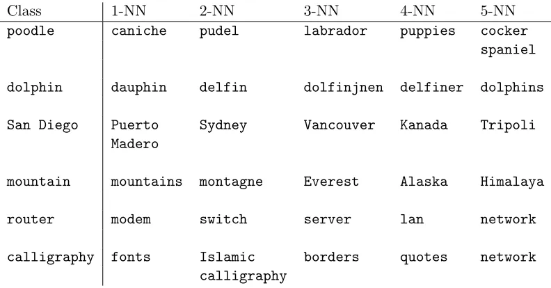
Table 7 gives examples of the classes corresponding to neighboring{βg}in the embedded feature space after the Wsabie++ training.
Class 1-NN 2-NN 3-NN 4-NN 5-NN
poodle caniche pudel labrador puppies cocker
spaniel
dolphin dauphin delfin dolfinjnen delfiner dolphins
San Diego Puerto Sydney Vancouver Kanada Tripoli
Madero
mountain mountains montagne Everest Alaska Himalaya
router modem switch server lan network
calligraphy fonts Islamic borders quotes network
calligraphy
Table 7: For each of the classes on the left, the table shows the five nearest (in terms of Euclidean distance) class prototypes{βg}in the proposed discriminatively trained embedded feature space for 21k Web Data set. Because these classes originated as web queries, some class names are translations of each other, for exampledolphin and dauphin(French for dolphin). While these may seem like exact synonyms, in fact different language communities often have slightly different visual notions of the same concept. Similarly, the classesObamaandPresident Obamaare expected to be largely overlapping, but their class distributions differ in the formality and context of the images.
parameters chosen using the validation set, and 10 last violators:
Number of Embedding Dimensions: 128 192 256 384 512 768 1024
Wsabie++ Test Accuracy: 7.4% 7.7% 8.3% 7.9% 7.1% 6.7% 6.5%
9.2 Comparison of Different Classifiers
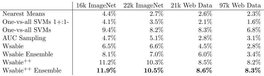
Table 8 compares the accuracy of the different classifiers, where all hyperparameters were cross-validated. The validated parameter choices are reported in Table 9.2
Wsabie++ was consistently most accurate, followed by the one-vs-all SVMs with the average number of negative samples per positive sample chosen by validation. The row labelled Wsabie++ was 2−26% more accurate and 2−4×more efficient (2−4× smaller model size) than the one-vs-all SVMs because the validated embedding dimension was 192 or 256 dimensions, down from the original 479 or 1024 features.
Like Perronnin et al. (2012), our experiments showed that choosing the hyperparameter of how many negative samples per positive sample for the one-vs-all SVMs made an im-pressive difference to its performance. The one-vs-all SVMs 1+:1-, which used a fixed ratio of one negative sample per positive sample was 2−4 times worse!
The row labelled Wsabie++ Ensemble is a concatenation of 2-4 Wsabie++ classifiers trained on different random samplings so that the total number of parameters is roughly the same as the SVM (the embedding matrices W add slightly to the total storage and efficiency calculations). With efficiency thus roughly controlled, the accuracy gain increased slightly to 3−28%.
The least improvement was seen on the 21k Web Data set. Our best hypothesis as to why that is that the classifiers are already close to the best performance possible with linear separators, and so there is little headroom for improvement. Some support for this hypoth-esis is the tiny gain the ensemble of multiple Wsabie++ classifiers versus the Wsabie++.
One surprise was that Wsabie++ performed almost as well on the 97k Web Data as on the 21k Web Data set even though there were four times as many classes. We have two main hypotheses of why this happened. First, there were more training samples in the 97k Web Data for the classes that were already present in the 21k Web Data. Second, the added classes had fewer samples but were often quite specific, and the samples from a specific class can be easier to distinguish than samples from a more generic class. For example, samples from the more specific class of diamond earrings are easier to distinguish than samples from the more generic classjewelry. Likewise, samples from the classbeer foamare easier to correctly classify than samples from the class beer.
10. Discussion, Hypotheses and Key Issues
This paper focused on how highly confusable classes can distort the empirical loss used in discriminative training of multi-class classifiers. We proposed a lightweight online approach to reduce the effect of highly-confusable classes on the empirical loss, and showed that it can
16k ImageNet 22k ImageNet 21k Web Data 97k Web Data
Nearest Means 4.4% 2.7% 2.6% 2.3%
One-vs-all SVMs 1+:1- 4.1% 3.5% 2.1% 1.6%
One-vs-all SVMs 9.4% 8.2% 8.3% 6.8%
AUC Sampling 4.7% 5.1% 2.8% 3.1%
Wsabie 6.5% 6.6% 4.5% 2.8%
Wsabie Ensemble 8.1% 7.0% 6.0% 3.4%
Wsabie++ 11.2% 10.3% 8.5% 8.2%
Wsabie++ Ensemble 11.9% 10.5% 8.6% 8.3%
Table 8: Image classification test accuracy
substantially increase performance in practice. Experimentally, we also showed that using adagrad to evolve the learning rates in the stochastic gradient descent is effective despite the nonconvexity of the loss (due to the joint learning of the linear dimensionality reduction and linear classifiers).
We argued that when there are many classes it is suboptimal to measure performance by simply counting errors, because this overemphasizes the noise of highly-confusable classes. Yet our test error is measured in the standard way: by counting how many samples were classified incorrectly. A better approach to measuring test error would be subjective judge-ments of error. In fact, we have verified that for the image classification problems consid-ered in the experiments, subjects are less critical about confusions of classes they consider more confusable (for example confusingdolphinandporpoise), but very critical of confu-sions between classes they do not consider confusable (for exampledolphinandStatue of Liberty). Thus, suppose you had two candidate classifiers, each of which made 100 errors, but one made all 100 errors betweendolphin and porpoiseand the other made 100 more random errors. Standard test error of summing the errors would consider these classifiers equal, but users would generally prefer the first classifier. Weston et al. (2011) provide one approach to addressing this issue with a sibling precision measure.
A related issue is that it is known that the experimental data sets used are not tagged with the complete set of correct class labels for each image. For example, in the 21k Web Data, an image of a red heart might be labelledloveandred, but not happen to be labelled heart, even though that would be considered a correct label in a subjective evaluation. We hypothesize that the proposed approach of probabilistically ignoring samples with consistent confusions helps reduce the impact of such missing positive labels.
Stepsize Margin Embedding Balance # LVs
dimension β
One-vs-all SVM
1+:1-16k ImageNet .01 .1
21k ImageNet .01 .1
21k Web Data .1 1
97k Web Data .01 .1
One-vs-all SVM
16k ImageNet .01 .1 64
21k ImageNet .01 .1 64
21k Web Data .1 1 64
97k Web Data .01 .1 128
AUC Sampling
16k ImageNet .01 .1
21k ImageNet .01 .1
21k Web Data .001 .01
97k Web Data .001 .01
Wsabie
16k ImageNet .01 .1 128
21k ImageNet .001 .1 128
21k Web Data .001 .1 256
97k Web Data .0001 .1 256
Wsabie++:
16k ImageNet 10 10,000 192 8
21k ImageNet 10 10,000 192 8
21k Web Data 10 10,000 256 8
97k Web Data 10 10,000 256 32
Table 9: Classifier parameters chosen using validation set
to consider for each positive class, rather than the WARP sampling which draws negative classes until it finds a violator. Preliminary results showed that the validation set chose the largest parameter choice which was almost the same as the number of classes. Thus that approach required another hyperparameter but seemed to be doing exactly what WARP sampling does and appeared to offer no accuracy improvement over WARP sampling.
WARP sampling strategy across multiple cores and multiple machines, but the details are outside the scope of this work.
Our experiments were some of the largest image labeling experiments ever performed, and were carefully implemented and executed. But our experiments were narrow and lim-ited in the sense that only image labeling problems were considered, and that the feature derivations were similar and all dense. The presented theory and motivation was not lim-ited however, and we hypothesize that similar results would hold up for other applications, different features, and sparser features.
We focused in this paper only on classifiers that use linear (or Euclidean) discriminant functions because they are popular for large-scale highly multiclass problems due to their efficiency and reasonably good performance. However, for a given feature set, the best performance on large data sets such as ImageNet may well be achieved with exact k-NN (Deng et al., 2010; Weston et al., 2013b) or a more sophisticated lazy classifier (Garcia et al., 2010), or with a deep network (Krizhevsky et al., 2012; Dean et al., 2012). However, for many real-life large-scale problems these methods may require infeasible memory and test-time, and so linear methods are of interest at least for their efficiency, and may be used to filter candidates to a smaller set for secondary evaluation by a more flexible classifier. In addition, the last layer of a neural network is often a linear or other high-model-bias classifier, and the proposed approaches may thus be useful in training a deep network as well.
Label trees and label partitioning can be even more efficient at inference (Bengio et al., 2010; Deng et al., 2011; Weston et al., 2013a). We did not take advantage or impose a hierarchical structure on the classes, which can be a fruitful approach to efficiently imple-menting highly multiclass classification. Other research in large-scale classification takes advantage of the natural hierarchy of classes in real-world classification problems such as labeling images (Deng et al., 2010; Griffin and Perona, 2008; Nister and Stewenius, 2006). For example, in Web Data one class iswedding cake, which could fit into the broader class of cake, and the even broader class of food. One problem with leveraging such hierarchies may be that they are not strict trees; wedding cake also falls under the broader class of wedding, or there may be no natural hierarchy. Some of the theory and strategy of this paper should be complementary to such hierarchical approaches.
Acknowledgments
We thank Mouhamadou Cisse, Gal Chechik, Andrew Cotter, Koby Crammer, John Duchi, Bela Frigyik, and Yoram Singer for helpful discussions.
Appendix: Proof of Proposition 1
LetZtbe a Bernoulli random variable with parameter pthat models the event that thetth sample of class y+ is classified as class h. Then for n trials the expected number of times a classy+ sample is classified as class h is E[P
tZt] =PtE[Zt] =nE[Zt] =np theZt are independent and identically distributed.
LetOtbe another Bernoulli random variable such thatOt= 1 if thetth sample of class
t >1,Ot= 1 iff Zt= 1 and Zt−1 = 0. Thus,
E[Ot] =E[Zt= 1 andZt−1 = 0] =P(Zt= 1, Zt−1 = 0) =P(Zt= 1)P(Zt= 0) =p(1−p) by the independence of the Bernoulli random variables Zt and Zt−1. Then the expected
number of confusions counted by (14) is E[P
tOt] = PtE[Ot] by linearity, which can be expanded: E[O1] +Pnt=2E[Ot] =p+ (n−1)p(1−p).
References
E. L. Allwein, R. E. Schapire, and Y. Singer. Reducing multiclass to binary: a unifying approach for margin classifiers. Journal Machine Learning Research, 1:113–141, 2000.
A. Barla, F. Odone, and A. Verri. Histogram intersection kernel for image classification.
Intl. Conf. Image Processing (ICIP), 3:513–516, 2003.
S. Bengio, J. Weston, and D. Grangier. Label embedding trees for large multi-class tasks. In NIPS, 2010.
Y. Bengio. Learning deep architectures for AI. Foundations and Trends in Machine Learn-ing, 2(1):1–127, 2009.
Y. Bengio, J. Laouradour, R. Collobert, and J. Weston. Curriculum learning. In ICML, 2009.
E. J. Bredensteiner and K. P. Bennet. Multicategory classification by support vector ma-chines. Computational Optimization and Applications, 12:53–79, 1999.
L. D. Brown, T. T. Cai, and A. DasGupta. Interval estimation for a binomial proportion.
Statistical Science, 16(2):101–117, 2001.
K. Crammer and Y. Singer. On the algorithmic implementation of multiclass kernel-based vector machines. Journal Machine Learning Research, 2001.
K. Crammer and Y. Singer. On the learnability and design of output codes for multiclass problems. Machine Learning, 47(2):201–233, 2002.
K. Crammer, O. Dekel, J. Keshet, S. Shalev-Shwartz, and Y. Singer. Online passive aggres-sive algorithms. Journal Machine Learning Research, 7:551–585, 2006.
A. Daniely, S. Sabato, and S. Shalev-Shwartz. Multiclass learning approaches: A theoretical comparison with implications. In NIPS, 2012.
J. Dean, G. S. Corrado, R. Monga, K. Chen, M. Devin, Q. V. Le, M. Z. Mao, M. Ranzato, A. Senoir, P. Tucker, K. Yang, and A. Ng. Large scale distributed deep networks. In
NIPS, 2012.
J. Deng, A. Berg, K. Li, and L. Fei-Fei. What does classifying more than 10,000 image categories tell us? In European Conf. Computer Vision (ECCV), 2010.
J. Deng, S. Satheesh, A. C. Berg, and L. Fei-Fei. Fast and balanced: Efficient label tree learning for large scale object recognition. InNIPS, 2011.
T. G. Dietterich and G. Bakiri. Solving multiclass learning problems via error-correcting output codes. Journal Artificial Intelligence Research, 2:264–286, 1995.
J. Duchi, E. Hazan, and Y. Singer. Adaptive subgradient methods for online learning and stochastic optimization. Journal Machine Learning Research, 12:2121–2159, 2011.
D. Eck. Personal communication from Google music expert Douglas Eck. 2013.
C. Fellbaum, editor. WordNet: An Electronic Lexical Database. MIT Press, 1998.
E. K. Garcia, S. Feldman, M. R. Gupta, and S. Srivastava. Completely lazy learning. IEEE Trans. Knowledge and Data Engineering, 22(9):1274–1285, 2010.
D. Grangier and S. Bengio. A discriminative kernel-based model to rank images from text queries. IEEE Trans. Pattern Analysis and Machine Intelligence, 30:1371–1384, 2008.
K. Grauman and T. Darrell. The pyramid match kernel: Efficient learning with sets of features. Journal Machine Learning Research, 8:725–760, April 2007.
G. Griffin and P. Perona. Learning and using taxonomies for fast visual categorization. In
CVPR, 2008.
Y. Guermeur. Combining discriminant models with new multi-class SVMs.Pattern Analysis and Applications, 5:168–179, 2002.
P. Hall and J. S. Marron. Geometric representation of high dimension, low sample size data.
J. R. Statst. Soc. B, 67(3):427–444, 2005.
T. Hastie, R. Tibshirani, and J. Friedman. The Elements of Statistical Learning. Springer-Verlag, New York, 2001.
R. Herbrich, T. Graepel, and K. Obermayer. Large margin rank boundaries for ordinal regression. In Advances in Large Margin Classifiers, pages 115–132. MIT Press, 2000.
A. Krizhevsky, I. Sutskever, and G. E. Hinton. ImageNet classification with deep convolu-tional neural networks. InNIPS, 2012.
Y. Lee, Y. Lin, and G. Wahba. Multicategory support vector machines. Journal American Statistical Association, 99(465):67–81, 2004.
T. Leung and J. Malik. Recognizing surface using three-dimensional textons. Intl. Conf. Computer Vision (ICCV), 1999.
M. Mohri, A. Rostamizadeh, and A. Talwalkar. Foundations of Machine Learning. MIT Press, Cambridge, MA, 2012.
Y. Mroueh, T. Poggio, L. Rosasco, and J-J E. Slotine. Multiclass learning with simplex coding. InNIPS, 2012.
D. Nister and H. Stewenius. Scalable recognition with a vocabulary tree. InCVPR, 2006.
A. Paton, N. Brummitt, R. Govaerts, K. Harman, S. Hinchcliffe, B. Allkin, and E. Lughadha. Target 1 of the global strategy for plant conservation: a working list of all known plant speciesprogress and prospects. Taxon, 57:602–611, 2008.
F. Perronnin, Z. Akata, Z. Harchaoui, and C. Schmid. Towards good practice in large-scale learning for image classification. In CVPR, 2012.
R. Rifkin and A. Klatau. In defense of one-vs-all classification. Journal Machine Learning Research, 5:101–141, 2004.
J. Sanchez and F. Perronnin. High-dimensional signature compression for large-scale image classification. In CVPR, 2011.
B. Schoelkopf, A. J. Smola, and K. R. M¨uller. Kernel principal component analysis. Ad-vances in kernel methods: support vector learning, pages 327–352, 1999.
O. Shamir and O. Dekel. Multiclass-multilabel classication with more classes than examples. In Proc. AISTATS, 2010.
A. Statnikov, C. F. Aliferis, I. Tsamardinos, D. Hardin, and S. Levy. A comprehensive evaluation of multicategory classification methods for microarray gene expression cancer diagnosis. Bioinformatics, 21(5):631–643, 2005.
A. Tewari and P. L. Bartlett. On the consistency of multiclass classification methods.
Journal Machine Learning Research, 2007.
N. Usunier, D. Buffoni, and P. Gallinari. Ranking with ordered weighted pairwise classifi-cation. In ICML, 2009.
V. Vapnik. Statistical Learning Theory. 1998.
J. Weston and C. Watkins. Multi-class support vector machines. Technical Report CSD-TR-98-04 Dept. Computer Science, Royal Holloway, University London, 1998.
J. Weston and C. Watkins. Support vector machines for multi-class pattern recognition. In
Proc. European Symposium on Artificial Neural Networks, 1999.
J. Weston, S. Bengio, and N. Usunier. Wsabie: Scaling up to large vocabulary image annotation. In Intl. Joint Conf. Artificial Intelligence, (IJCAI), pages 2764–2770, 2011.
J. Weston, R. Weiss, and H. Yee. Affinity weighted embedding. InProc. International Conf. Learning Representations, 2013b.
L. Xiao. Dual averaging methods for regularized stochastic learning and online optimization.
Microsoft Research Technical Report MSR-TR-2010-23, 2010.
T. Zhang. Statistical analysis of some multi-category large margin classification methods.