Relational Dependency Networks

Relational Dependency Networks

Jennifer Neville [email protected]

Departments of Computer Science and Statistics Purdue University

West Lafayette, IN 47907-2107, USA

David Jensen [email protected]

Department of Computer Science University of Massachusetts Amherst Amherst, MA 01003-4610, USA

Editor: Max Chickering

Abstract

Recent work on graphical models for relational data has demonstrated significant improvements in classification and inference when models represent the dependencies among instances. Despite its use in conventional statistical models, the assumption of instance independence is contradicted by most relational data sets. For example, in citation data there are dependencies among the topics of a paper’s references, and in genomic data there are dependencies among the functions of interacting proteins. In this paper, we present relational dependency networks (RDNs), graphical models that are capable of expressing and reasoning with such dependencies in a relational setting. We discuss RDNs in the context of relational Bayes networks and relational Markov networks and outline the relative strengths of RDNs—namely, the ability to represent cyclic dependencies, simple methods for parameter estimation, and efficient structure learning techniques. The strengths of RDNs are due to the use of pseudolikelihood learning techniques, which estimate an efficient approximation of the full joint distribution. We present learned RDNs for a number of real-world data sets and eval-uate the models in a prediction context, showing that RDNs identify and exploit cyclic relational dependencies to achieve significant performance gains over conventional conditional models. In addition, we use synthetic data to explore model performance under various relational data char-acteristics, showing that RDN learning and inference techniques are accurate over a wide range of conditions.

Keywords: relational learning, probabilistic relational models, knowledge discovery, graphical models, dependency networks, pseudolikelihood estimation

1. Introduction

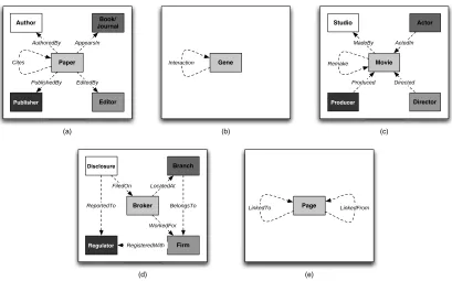
The presence of autocorrelation provides a strong motivation for using relational techniques for learning and inference. Autocorrelation is a statistical dependency between the values of the same variable on related entities and is a nearly ubiquitous characteristic of relational data sets (Jensen and Neville, 2002). For example, hyperlinked web pages are more likely to share the same topic than randomly selected pages. More formally, we define relational autocorrelation with respect to an attributed graph G= (V,E), where each node v∈V represents an object and each edge e∈E

represents a binary relation. Autocorrelation is measured for a set of instance pairs PR related

through paths of length l in a set of edges ER: PR={(vi,vj): eik1,ek1k2, ...,eklj∈ER}, where ER=

{ei j} ⊆E. It is the correlation between the values of a variable X on the instance pairs(vi.x,vj.x)

such that(vi,vj)∈PR. Recent analyses of relational data sets have reported autocorrelation in the

following variables:

• Topics of hyperlinked web pages (Chakrabarti et al., 1998; Taskar et al., 2002),

• Industry categorization of corporations that share board members (Neville and Jensen, 2000),

• Fraud status of cellular customers who call common numbers (Fawcett and Provost, 1997; Cortes et al., 2001),

• Topics of coreferent scientific papers (Taskar et al., 2001; Neville and Jensen, 2003),

• Functions of colocated proteins in a cell (Neville and Jensen, 2002),

• Box-office receipts of movies made by the same studio (Jensen and Neville, 2002),

• Industry categorization of corporations that co-occur in news stories (Bernstein et al., 2003),

• Tuberculosis infection among people in close contact (Getoor et al., 2001), and

• Product/service adoption among customers in close communication (Domingos and Richard-son, 2001; Hill et al., 2006).

When relational data exhibit autocorrelation there is a unique opportunity to improve model performance because inferences about one object can inform inferences about related objects. In-deed, recent work in relational domains has shown that collective inference over an entire data set results in more accurate predictions than conditional inference for each instance independently (e.g., Chakrabarti et al., 1998; Neville and Jensen, 2000; Lu and Getoor, 2003), and that the gains over conditional models increase as autocorrelation increases (Jensen et al., 2004).

Joint relational models are able to exploit autocorrelation by estimating a joint probability distri-bution over an entire relational data set and collectively inferring the labels of related instances. Re-cent research has produced several novel types of graphical models for estimating joint probability distributions for relational data that consist of non-independent and heterogeneous instances (e.g., Getoor et al., 2001; Taskar et al., 2002). We will refer to these models as probabilistic relational

domains, removing the assumption of independent and identically distributed instances that under-lies conventional learning techniques.2 PRMs have been successfully evaluated in several domains, including the World Wide Web, genomic data, and scientific literature.

Directed PRMs, such as relational Bayes networks3(RBNs) (Getoor et al., 2001), can model au-tocorrelation dependencies if they are structured in a manner that respects the acyclicity constraint of the model. While domain knowledge can sometimes be used to structure the autocorrelation dependencies in an acyclic manner, often an acyclic ordering is unknown or does not exist. For ex-ample, in genetic pedigree analysis there is autocorrelation among the genes of relatives (Lauritzen and Sheehan, 2003). In this domain, the casual relationship is from ancestor to descendent so we can use the temporal parent-child relationship to structure the dependencies in an acyclic manner (i.e., parents’ genes will never be influenced by the genes of their children). However, given a set of hyperlinked web pages, there is little information to use to determine the causal direction of the dependency between their topics. In this case, we can only represent the autocorrelation between two web pages as an undirected correlation. The acyclicity constraint of directed PRMs precludes the learning of arbitrary autocorrelation dependencies and thus severely limits the applicability of these models in relational domains.4

Undirected PRMs, such as relational Markov networks (RMNs) (Taskar et al., 2002), can rep-resent and reason with arbitrary forms of autocorrelation. However, research on these models has focused primarily on parameter estimation and inference procedures. Current implementations of RMNs do not select features—model structure must be pre-specified by the user. While, in prin-ciple, it is possible for RMN techniques to learn cyclic autocorrelation dependencies, inefficient parameter estimation makes this difficult in practice. Because parameter estimation requires multi-ple rounds of inference over the entire data set, it is impractical to incorporate it as a subcomponent of feature selection. Recent work on conditional random fields for sequence analysis includes a feature selection algorithm (McCallum, 2003) that could be extended for RMNs. However, the algorithm abandons estimation of the full joint distribution and uses pseudolikelihood estimation, which makes the approach tractable but removes some of the advantages of reasoning with the full joint distribution.

In this paper, we outline relational dependency networks (RDNs),5an extension of dependency networks (Heckerman et al., 2000) for relational data. RDNs can represent and reason with the cyclic dependencies required to express and exploit autocorrelation during collective inference. In this regard, they share certain advantages of RMNs and other undirected models of relational data (Chakrabarti et al., 1998; Domingos and Richardson, 2001; Richardson and Domingos, 2006). To our knowledge, RDNs are the first PRM capable of learning cyclic autocorrelation dependen-cies. RDNs also offer a relatively simple method for structure learning and parameter estimation, which results in models that are easier to understand and interpret. In this regard, they share cer-tain advantages of RBNs and other directed models (Sanghai et al., 2003; Heckerman et al., 2004).

2. Another class of joint models extend conventional logic programming models to support probabilistic reasoning in first-order logic environments (Kersting and Raedt, 2002; Richardson and Domingos, 2006). We refer to these models as probabilistic logic models (PLMs). See Section 5.2 for more detail.

3. We use the term relational Bayesian network to refer to Bayesian networks that have been upgraded to model re-lational databases. The term has also been used by Jaeger (1997) to refer to Bayesian networks where the nodes correspond to relations and their values represent possible interpretations of those relations in a specific domain. 4. The limitation is due to the PRM modeling approach (see Section 3.1), which ties parameters across items of the same

The primary distinction between RDNs and other existing PRMs is that RDNs are an approximate model. RDNs approximate the full joint distribution and thus are not guaranteed to specify a con-sistent probability distribution. The quality of the approximation will be determined by the data available for learning—if the models are learned from large data sets, and combined with Monte Carlo inference techniques, the approximation should be sufficiently accurate.

We start by reviewing the details of dependency networks for propositional data. Then we describe the general characteristics of PRMs and outline the specifics of RDN learning and inference procedures. We evaluate RDN learning and inference on synthetic data sets, showing that RDN learning is accurate for large to moderate-sized data sets and that RDN inference is comparable, or superior, to RMN inference over a range of data conditions. In addition, we evaluate RDNs on five real-world data sets, presenting learned RDNs for subjective evaluation. Of particular note, all the real-world data sets exhibit multiple autocorrelation dependencies that were automatically discovered by the RDN learning algorithm. We evaluate the learned models in a prediction context, where only a single attribute is unobserved, and show that the models outperform conventional conditional models on all five tasks. Finally, we review related work and conclude with a discussion of future directions.

2. Dependency Networks

Graphical models represent a joint distribution over a set of variables. The primary distinction be-tween Bayesian networks, Markov networks, and dependency networks (DNs) is that dependency networks are an approximate representation. DNs approximate the joint distribution with a set of conditional probability distributions (CPDs) that are learned independently. This approach to learn-ing results in significant efficiency gains over exact models. However, because the CPDs are learned independently, DNs are not guaranteed to specify a consistent6joint distribution, where each CPD can be derived from the joint distribution using the rules of probability. This limits the applicability of exact inference techniques. In addition, the correlational DN representation precludes DNs from being used to infer causal relationships. Nevertheless, DNs can encode predictive relationships (i.e., dependence and independence) and Gibbs sampling inference techniques (e.g., Neal, 1993) can be used to recover a full joint distribution, regardless of the consistency of the local CPDs. We begin by reviewing traditional graphical models and then outline the details of dependency networks in this context.

Consider the set of variables X = (X1, ...,Xn) over which we would like to model the joint distribution p(x) =p(x1, ...,xn). We use upper case letters to refer to random variables and lower

case letters to refer to an assignment of values to the variables.

A Bayesian network for X uses a directed acyclic graph G= (V,E) and a set of conditional probability distributions P to represent the joint distribution over X. Each node v∈V corresponds

to an Xi ∈X. The edges of the graph encode dependencies among the variables and can be used

to infer conditional independence among variables using notions of d-separation. The parents of node Xi, denoted PAi, are the set of vj∈V such that(vj,vi)∈E. The set P contains a conditional

probability distribution for each variable given its parents, p(xi|pai). The acyclicity constraint on G ensures that the CPDs in P factor the joint distribution into the formula below. A directed graph is acyclic if there is no directed path that starts and ends at the same variable. More specifically, there

can be no self-loops from a variable to itself. Given(G,P), the joint probability for a set of values x is computed with the formula:

p(x) =

n

∏

i=1

p(xi|pai).

A Markov network for X uses an undirected graph U = (V,E)and a set of potential functions

Φto represent the joint distribution over X. Again, each node v∈V corresponds to an Xi∈X and

the edges of the graph encode conditional independence assumptions. However, with undirected graphs, conditional independence can be inferred using simple graph separation. Let C(U)be the set of cliques in the graph U . Then each clique c∈C(U) is associated with a set of variables Xc

and a clique potentialφc(xc)which is a non-negative function over the possible values for xc. Given

(U,Φ), the joint probability for a set of values x is computed with the formula:

p(x) = 1

Z c

∏

i=1

φi(xci),

where Z=∑_X∏c

i=1φi(xci)is a normalizing constant, which sums over all possible instantiations of

x to ensure that p(x)is a true probability distribution.

2.1 DN Representation

Dependency networks are an alternative form of graphical model that approximates the full joint distribution with a set of conditional probability distributions that are each learned independently. A DN encodes probabilistic relationships among a set of variables X in a manner that combines characteristics of both undirected and directed graphical models. Dependencies among variables are represented with a directed graph G= (V,E), where conditional independence is interpreted using graph separation, as with undirected models. However, as with directed models, dependencies are quantified with a set of conditional probability distributions P. Each node vi ∈V corresponds

to an Xi ∈X and is associated with a probability distribution conditioned on the other variables, P(vi) = p(xi|x− {xi}). The parents of node i are the set of variables that render Xi conditionally

independent of the other variables (p(xi|pai) = p(xi|x− {xi})), and G contains a directed edge from each parent node vj to each child node vi ((vj,vi)∈E iff Xj ∈pai). The CPDs in P do not

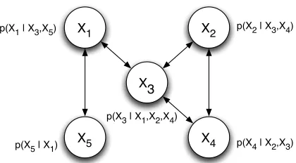
necessarily factor the joint distribution so we cannot compute the joint probability for a set of values x directly. However, given G and P, a joint distribution can be recovered through Gibbs sampling (see Section 3.4 for details). From the joint distribution, we can extract any probabilities of interest. For example, the DN in Figure 1 models the set of variables: X={X1,X2,X3,X4,X5}. Each

node is conditionally independent of the other nodes in the graph given its immediate neighbors (e.g., X1 is conditionally independent of {X2,X4} given {X3,X5}). Each node contains a CPD,

which specifies a probability distribution over its possible values, given the values of its parents.

2.2 DN Learning

Both the structure and parameters of DNs are determined through learning the local CPDs. The DN learning algorithm learns a separate distribution for each variable Xi, conditioned on the other

variables in the data (i.e., X− {Xi}). Any conditional learner can be used for this task (e.g., logistic

X₁

X₃

X₂

X₄

X_{5 p ( X}

4 | X2, X3) p ( X₂ | X₃, X₄)

p ( X₅ | X₁) p ( X₁ | X₃, X₅)

p ( X₃ | X₁, X₂, X₄)

Figure 1: Example dependency network.

The parents are then reflected in the edges of G appropriately. If the conditional learner is not selective (i.e., the algorithm does not select a subset of the features), the DN will be fully connected (i.e., PAi=x− {xi}). In order to build understandable DNs, it is desirable to use a selective learner

that will learn CPDs that use a subset of all available variables.

2.3 DN Inference

Although the DN approach to structure learning is simple and efficient, it can result in an inconsis-tent network, both structurally and numerically. In other words, there may be no joint distribution from which each of the CPDs can be obtained using the rules of probability. Learning the CPDs in-dependently with a selective conditional learner can result in a network that contains a directed edge from Xito Xj, but not from Xjto Xi. This is a structural inconsistency—Xiand Xjare dependent but Xj is not represented in the CPD for Xi. In addition, learning the CPDs independently from finite

samples may result in numerical inconsistencies in the parameter estimates. If this is the case, the joint distribution derived numerically from the CPDs will not sum to one. However, when a DN is inconsistent, approximate inference techniques can still be used to estimate a full joint distribution and extract probabilities of interest. Gibbs sampling can be used to recover a full joint distribution, regardless of the consistency of the local CPDs, provided that each Xi is discrete and its CPD is

positive (Heckerman et al., 2000). In practice, Heckerman et al. (2000) show that DNs are nearly consistent if learned from large data sets because the data serve a coordinating function to ensure some degree of consistency among the CPDs.

3. Relational Dependency Networks

Several characteristics of DNs are particularly desirable for modeling relational data. First, learning a collection of conditional models offers significant efficiency gains over learning a full joint model. This is generally true, but it is even more pertinent to relational settings where the feature space is very large. Second, networks that are easy to interpret and understand aid analysts’ assessment of the utility of the relational information. Third, the ability to represent cycles in a network facilitates reasoning with autocorrelation, a common characteristic of relational data. In addition, whereas the need for approximate inference is a disadvantage of DNs for propositional data, due to the complexity of relational model graphs in practice, all PRMs use approximate inference.

Relational dependency networks extend DNs to work with relational data in much the same way that RBNs extend Bayesian networks and RMNs extend Markov networks.7 These extensions take

a graphical model formalism and upgrade (Kersting, 2003) it to a first-order logic representation with an entity-relationship model. We start by describing the general characteristics of probabilistic relational models and then discuss the details of RDNs in this context.

3.1 Probabilistic Relational Models

PRMs represent a joint probability distribution over the attributes of a relational data set. When modeling propositional data with a graphical model, there is a single graph G that comprises the model. In contrast, there are three graphs associated with models of relational data: the data graph

GD, the model graph GM, and the inference graph GI. These correspond to the skeleton, model, and ground graph as outlined in Heckerman et al. (2004).

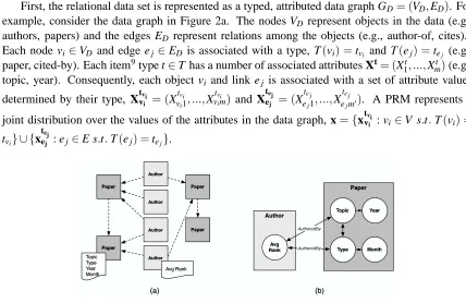
First, the relational data set is represented as a typed, attributed data graph GD= (VD,ED). For

example, consider the data graph in Figure 2a. The nodes VD represent objects in the data (e.g.,

authors, papers) and the edges ED represent relations among the objects (e.g., author-of, cites).8

Each node vi ∈VD and edge ej ∈ED is associated with a type, T(vi) =tvi and T(ej) =tej (e.g.,

paper, cited-by). Each item9type t∈T has a number of associated attributes Xt= (X₁t, ...,X_mt)(e.g., topic, year). Consequently, each object vi and link ej is associated with a set of attribute values

determined by their type, Xtvvii = (X

t_vi vi1, ...,X

t_vi

vim) and X

t_ej ej = (X

t_{e j} ej1, ...,X

t_{e j}

ejm0). A PRM represents a

joint distribution over the values of the attributes in the data graph, x={xtvvii : vi∈V s.t.T(vi) =

tvi} ∪ {x

t_ej

ej : ej∈E s.t.T(ej) =tej}.

!" #%$ #& '( )& *,+&-./0

1&23 4 5 6789:

6;%8%< =<>?

@A7BCD E&F%GH

>BI

AuthoredBy

AuthoredBy

Figure 2: Example (a) data graph and (b) model graph.

Next, the dependencies among attributes are represented in the model graph GM= (VM,EM).

Attributes of an item can depend probabilistically on other attributes of the same item, as well as on attributes of other related objects or links in GD. For example, the topic of a paper may be

influenced by attributes of the authors that wrote the paper. The relations in GD are used to limit

the search for possible statistical dependencies, thus they constrain the set of edges that can appear in GM. However, note that a relationship between two objects in GD does not necessarily imply a

probabilistic dependence between their attributes in GM.

Instead of defining the dependency structure over attributes of specific objects, PRMs define a generic dependency structure at the level of item types. Each node v∈VM corresponds to an X_kt,

8. We use rectangles to represent objects, circles to represent random variables, dashed lines to represent relations, and solid lines to represent probabilistic dependencies.

where t∈T ∧ X_kt ∈Xt. The set of attributes Xt_k= (X_ikt :(vi∈V ∨ ei ∈E) ∧ T(i) =t) is tied together and modeled as a single variable. This approach of typing items and tying parameters across items of the same type is an essential component of PRM learning. It enables generalization from a single instance (i.e., one data graph) by decomposing the data graph into multiple examples of each item type (e.g., all paper objects), and building a joint model of dependencies between and among attributes of each type.

As in conventional graphical models, each node is associated with a probability distribution conditioned on the other variables. Parents of X_kt are either: (1) other attributes associated with items of type tk (e.g., paper topic depends on paper type), or (2) attributes associated with items of

type tjwhere items tjare related to items tkin GD(e.g., paper topic depends on author rank). For the

latter type of dependency, if the relation between tkand tjis one-to-many, the parent consists of a set

of attribute values (e.g., author ranks). In this situation, current PRMs use aggregation functions to generalize across heterogeneous attributes sets (e.g., one paper may have two authors while another may have five). Aggregation functions are used to either map sets of values into single values, or to combine a set of probability distributions into a single distribution.

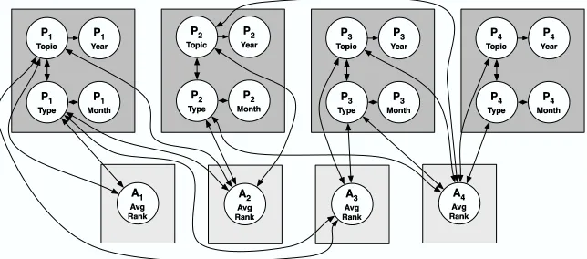
Consider the RDN model graph GM in Figure 2b.10 It models the data in Figure 2a, which

has two object types: paper and author. In GM, each item type is represented by a plate, and each

attribute of each item type is represented as a node. Edges characterize the dependencies among the attributes at the type level. The representation uses a modified plate notation. Dependencies among attributes of the same object are represented by arcs within a rectangle; arcs that cross rectangle boundaries represent dependencies among attributes of related objects, with edge labels indicating the underlying relations. For example, monthi depends on typei, while avgrankj depends on the typek and topickfor all papers k written by author j in GD.

There is a nearly limitless range of dependencies that could be considered by algorithms for learning PRMs. In propositional data, learners model a fixed set of attributes intrinsic to each object. In contrast, in relational data, learners must decide how much to model (i.e., how much of the relational neighborhood around an item can influence the probability distribution of an item’s attributes). For example, a paper’s topic may depend of the topics of other papers written by its authors—but what about the topics of the references in those papers or the topics of other papers written by coauthors of those papers? Two common approaches to limiting search in the space of relational dependencies are: (1) exhaustive search of all dependencies within a fixed-distance neighborhood in GD(e.g., attributes of items up to k links away), or (2) greedy iterative-deepening

search, expanding the search in GDin directions where the dependencies improve the likelihood.

Finally, during inference, a PRM uses a model graph GMand a data graph GDto instantiate an

inference graph GI= (VI,VE)in a process sometimes called “roll out.” The roll out procedure used

by PRMs to produce GI is nearly identical to the process used to instantiate sequence models such

as hidden Markov models. GI represents the probabilistic dependencies among all the variables in

a single test set (here GD is usually different from GD0 used for training). The structure of GI is

determined by both GDand GM—each item-attribute pair in GDgets a separate, local copy of the

appropriate CPD from GM. The relations in GDdetermine the way that GMis rolled out to form GI.

PRMs can produce inference graphs with wide variation in overall and local structure because the structure of GIis determined by the specific data graph, which typically has non-uniform structure.

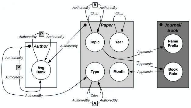
For example, Figure 3 shows the model from Figure 2b rolled out over the data set in Figure 2a.

Notice that there are a variable number of authors per paper. This illustrates why current PRMs use aggregation in their CPDs—for example, the CPD for paper-type must be able to deal with a variable number of author ranks.

! ! ! ! ! #" " " " "

Figure 3: Example inference graph.

3.2 RDN Representation

Relational dependency networks encode probabilistic relationships in a similar manner to DNs, extending the representation to a relational setting. RDNs use a directed model graph GM with a

set of conditional probability distributions P. Each node vi∈VM corresponds to an X_kt∈Xt, t∈T

and is associated with a conditional distribution p(xt_k|pa_xt

k). Figure 2b illustrates an example RDN

model graph for the data graph in Figure 2a. The graphical representation illustrates the qualitative component (GD) of the RDN—it does not depict the quantitative component (P) of the model, which

consists of CPDs that use aggregation functions. Although conditional independence is inferred using an undirected view of the graph, directed edges are useful for representing the set of variables in each CPD. For example, in Figure 2b the CPD for year contains topic but the CPD for topic does not contain year. This represents any inconsistencies that result from the RDN learning technique.

A consistent RDN specifies a joint probability distribution p(x) over the attribute values of a relational data set from which each CPD∈P can be derived using the rules of probability. There

is a direct correspondence between consistent RDNs and relational Markov networks. It is similar to the correspondence between consistent DNs and Markov networks (Heckerman et al., 2000), but the correspondence is defined with respect to the template model graphs GMand UM.

Theorem 1 The set of positive distributions that can be encoded by a consistent RDN(GM,P)is equal to the set of positive distributions that can be encoded by an RMN (UM,Φ) provided (1) GM=UM, and (2) P andΦuse the same aggregation functions.

Proof Let p be a positive distribution defined by an RMN (UM,Φ) for GD. First, we construct

a Markov network with tied clique potentials by rolling out the RMN inference graph UI over the

data graph GD. By Theorem 1 of Heckerman et al. (2000), which uses the Hammersley-Clifford

theorem (Besag, 1974), there is a corresponding dependency network that represents the same dis-tribution p as the Markov network UI. Since the conditional probability distribution for each

adjacent to each occurrence are equivalent by definition, thus by the global Markov property the derived CPDs will be identical. From this dependency network we can construct a consistent RDN

(GM,P)by first setting GM=UM. Next, we compute from UI the CPDs for the attributes of each

item type: p(xt_k|x− {xt_k})for t∈T,X_kt∈Xt. To derive the CPDs for P, the CPDs must use the same aggregation functions as the potentials inΦ. Since the adjacencies in the RDN model graph are the same as those in the RMN model graph, and there is a correspondence between the rolled out DN and MN, the distribution encoded by the RDN is p.

Next let p be a positive distribution defined by an RDN(GM,P)for GD. First, we construct a

dependency network with tied CPDs by rolling out the RDN inference graph GIover the data graph GD. Again, by Theorem 1 of Heckerman et al. (2000), there is a corresponding Markov network that

represents the same distribution p as the dependency network GI. Of the valid Markov networks

representing p, there will exist a network where the potentials are tied across occurrences of the same clique template (i.e.,∀ci∈C φC(xC)). This follows from the first part of the proof, which

shows that each RMN with tied clique potentials can be transformed to an RDN with tied CPDs. From this Markov network we can construct an RMN(UM,Φ)by setting UM=GM and grouping

the set of clique template potentials inΦ. Since the adjacencies in the RMN model graph are the same as those in the RDN model graph, and since there is a correspondence between the rolled out MN and DN, the distribution encoded by the RMN is p.

This proof shows an exact correspondence between consistent RDNs and RMNs. We cannot show the same correspondence for general RDNs. However, we will show in Section 3.4 that Gibbs sampling can be used to extract a unique joint distribution, regardless of the consistency of the model.

3.3 RDN Learning

Learning a PRM consists of two tasks: learning the dependency structure among the attributes of each object type, and estimating the parameters of the local probability models for an attribute given its parents. Relatively efficient techniques exist for learning both the structure and param-eters of RBNs. However, these techniques exploit the requirement that the CPDs factor the full distribution—a requirement that imposes acyclicity constraints on the model and precludes the learning of arbitrary autocorrelation dependencies. On the other hand, it is possible for RMN techniques to learn cyclic autocorrelation dependencies in principle. However, inefficiencies due to calculating the normalizing constant Z in undirected models make this difficult in practice. Cal-culation of Z requires a summation over all possible states x. When modeling the joint distribution of propositional data, the number of states is exponential in the number of attributes (i.e., O(2m)). When modeling the joint distribution of relational data, the number of states is exponential in the number of attributes and the number of instances. If there are N objects, each with m attributes, then the total number of states is O(2Nm). For any reasonable-size data set, a single calculation of Z is an enormous computational burden. Feature selection generally requires repeated parameter estimation while measuring the change in likelihood affected by each attribute, which would require recalculation of Z on each iteration.

auto-correlation dependencies. The pseudolikelihood for data graph GDis computed as a product over

the item types t, the attributes of that type Xt, and the items of that type v,e:

PL(GD;θ) =

∏

t∈TX

∏

∏

v:T(v)=t

p(xt_vi|paxt

vi;θ)

∏

e:T(e)=t

p(xt_ei|paxt

ei;θ). (1)

On the surface, Equation 1 may appear similar to a likelihood that specifies a joint distribution of an RBN. However, the CPDs in the RDN pseudolikelihood are not required to factor the joint distribution of GD. More specifically, when we consider the variable X_vit, we condition on the

values of the parents PA_Xt

vi regardless of whether the estimation of CPDs for variables in PAXvit was

conditioned on X_vit. The parents of X_vit may include other variables on the same item (e.g., X_vit0 such

that i0 6=i), the same variable on related items (e.g., X_vt0_i such that v0 6=v), or other variables on

related items (e.g., X_vt00_i0 such that v06=v and i06=i).

Pseudolikelihood estimation avoids the complexities of estimating Z and the requirement of acyclicity. Instead of optimizing the log-likelihood of the full joint distribution, we optimize the pseudo-loglikelihood. The contribution for each variable is conditioned on all other attribute values in the data, thus we can maximize the pseudo-loglikelihood for each variable independently:

log PL(GD;θ) =

∑

∑

i∈Xt

∑

v:T(v)=t

log p(xt_vi|pa_xt

vi;θ) +

∑

e:T(e)=t

log p(xt_ei|pa_xt ei;θ).

In addition, this approach can make use of existing techniques for learning conditional probability distributions of relational data such as first-order Bayesian classifiers (Flach and Lachiche, 1999), structural logistic regression (Popescul et al., 2003), or ACORA (Perlich and Provost, 2003).

Maximizing the pseudolikelihood function gives the maximum pseudolikelihood estimate (MPLE) ofθ. To estimate the parameters we need to solve the following pseudolikelihood equation:

∂

∂θPL(GD;θ) =0. (2)

With this approach we lose the asymptotic efficiency properties of maximum likelihood esti-mators. However, under some general conditions the asymptotic properties of the MPLE can be established. In particular, in the limit as sample size grows, the MPLE will be an unbiased estimate of the true parameterθ0and it will be normally distributed. Geman and Graffine (1987) established

the first proof of the properties of maximum pseudolikelihood estimators of fully observed data. Gidas (1986) gives an alternative proof and Comets (1992) establishes a more general proof that does not require a finite state space x or stationarity of the true distribution P_θ0.

Theorem 2 Assume the following regularity conditions11are satisfied for an RDN: 1. The model is identifiable (i.e., ifθ6=θ0, then PL(GD;θ)6=PL(GD;θ0)).

2. The distributions PL(GD;θ)have common support and are differentiable with respect toθ.

3. The parameter spaceΩcontains an open setωof which the true parameterθ0is an interior point.

In addition, assume the pseudolikelihood equation (Equation 2) has a unique solution inΩalmost surely as |GD| →∞. Then, provided that GD is of bounded degree, the MPLE ˜θ converges in probability to the true valueθ0as|GD| →∞.

Proof Provided the size of the RDN does not grow as the size of the data set grows (i.e., |P| re-mains constant as|GD| →∞) and GDis of bounded degree, then previous proofs apply. We provide

the intuition for the proof here and refer the reader to Comets (1992), White (1994), and Lehmann and Casella (1998) for details. Let ˜θbe the maximum pseudolikelihood estimate that maximizes

PL(GD;θ). As|GD| →∞, the data will consist of all possible data configurations for each CPD∈P

(assuming bounded degree structure in GD). As such, the pseudolikelihood function will converge

to its expectation, PL(GD;θ)→E(PL(GD;θ)). The expectation is maximized by the true parameter

θ0 because the expectation is taken with respect to all possible data configurations. Therefore as

|GD| →∞, the MPLE converges to the true parameter (i.e., ˜θ−θ0→0).

The RDN learning algorithm is similar to the DN learning algorithm, except we use a relational probability estimation algorithm to learn the set of conditional models, maximizing pseudolikeli-hood for each variable separately. The algorithm input consists of: (1) GD: a relational data graph,

(2) R: a conditional relational learner, and (3) Qt: a set of queries12 that specify the relational neighborhood considered in R for each type T .

Table 1 outlines the learning algorithm in pseudocode. The algorithm cycles over each attribute of each item type and learns a separate CPD, conditioned on the other values in the training data. We discuss details of the subcomponents (querying and relational learners) in the sections below.

The asymptotic complexity of RDN learning is O(|X| · |PAX| ·N), where|X|is the number of

CPDs to be estimated, |PAX|is the number of attributes and N is the number of instances, used to estimate the CPD for X .13 Quantifying the asymptotic complexity of RBN and RMN learning is difficult due to the use of heuristic search and numerical optimization techniques. RBN learning requires multiple rounds of parameter estimation during the algorithm’s heuristic search through the model space, and each round of parameter estimation has the same complexity as RDN learning, thus RBN learning will generally require more time. For RMN learning, there is no closed-form parameter estimation technique. Instead the models are trained using conjugate gradient, where each iteration requires approximate inference over the unrolled Markov network. In general this RMN nested loop of optimization and approximation will require more time to learn than an RBN (Taskar et al., 2002). Therefore, given equivalent search spaces, RMN learning is generally more complex than RBN learning, and RBN learning is generally more complex than RDN learning.

3.3.1 QUERIES

In our implementation, we use queries to specify the relational neighborhoods that will be con-sidered by the conditional learner R. The queries’ structures define a typing over instances in the database. Subgraphs are extracted from a larger graph database using the visual query language QGraph (Blau et al., 2001). Queries allow for variation in the number and types of objects and links that form the subgraphs and return collections of all matching subgraphs from the database.

12. Our implementation employs a set of user-specified queries to limit the search space considered during learning.

However, a simple depth limit (e.g.,≤2 links away in the data graph) can be used to limit the search space as well.

13. This assumes the complexity of the relational learner R is O(|PAX| ·N), which is true for the two relational learners

Learn RDN (GD,R,Qt): P←/0

For each t∈T :

For each X_kt ∈Xt:

Use R to learn a CPD for X_kt given the attributes in the relational neighborhood defined by Qt.

P←P∪CPD_Xt k

Use P to form GM.

Table 1: RDN learning algorithm.

Paper

A u t hor

Refer-ence

Refer-ence

Refer-ence

Refer-ence

Refer-ence

Refer-ence

Refer-ence A u t hor

Paper

A u t hor

Linktype=AuthorOf

Refer-ence

Linktype=Cites AND( Objecttype=Paper,

Year=1 9 9 5 )

Objecttype=Person

Objecttype=Paper [0 . . ] [0 . . ]

( a) ( b)

Paper. ID! =Reference. ID

Figure 4: (a) Example QGraph query: Textual annotations specify match conditions on attribute values; numerical annotations (e.g., [0..]) specify constraints on the cardinality of matched objects (e.g., zero or more authors), and (b) matching subgraph.

For example, consider the query in Figure 4a.14 The query specifies match criteria for a target item (paper) and its local relational neighborhood (authors and references). The example query matches all research papers that were published in 1995 and returns for each paper a subgraph that includes all authors and references associated with the paper. Note the constraint on paper ID in the lower left corner—this ensures that the target paper does not match as a reference in the resulting subgraphs. Figure 4b shows a hypothetical match to this query: a paper with two authors and seven references.

The query defines a typing over the objects of the database (e.g., people that have authored a paper are categorized as authors) and specifies the relevant relational context for the target item type in the model. For example, given this query the learner R would model the distribution of a paper’s attributes given the attributes of the paper itself and the attributes of its related authors and references. The queries are a means of restricting model search. Instead of setting a simple depth limit on the extent of the search, the analyst has a more flexible means with which to limit the search (e.g., we can consider other papers written by the paper’s authors but not other authors of the paper’s references).

3.3.2 CONDITIONALRELATIONALLEARNERS

The conditional relational learner R is used for both parameter estimation and structure learning in RDNs. The variables selected by R are reflected in the edges of GMappropriately. If R selects all of

the available attributes, the RDN will be fully connected.

In principle, any conditional relational learner can be used as a subcomponent to learn the indi-vidual CPDs provided that it can closely approximate CPDs consistent with the joint distribution. In this paper, we discuss the use of two different conditional models—relational Bayesian classifiers (RBCs) (Neville et al., 2003b) and relational probability trees (RPTs) (Neville et al., 2003a). Relational Bayesian Classifiers

RBCs extend Bayesian classifiers to a relational setting. RBCs treat heterogeneous relational sub-graphs as a homogenous set of attribute multisets. For example, when considering the references of a single paper, the publication dates of those references form multisets of varying size (e.g., {1995, 1995, 1996}, {1975, 1986, 1998, 1998}). The RBC assumes each value of a multiset is independently drawn from the same multinomial distribution.15 This approach is designed to mir-ror the independence assumption of the naive Bayesian classifier. In addition to the conventional assumption of attribute independence, the RBC also assumes attribute value independence within each multiset.

For a given item type t ∈T , the query scope specifies the set of item types TR that form the relevant relational neighborhood for t. Note that TR does not necessarily contain all item types

in the database and the query may also dynamically introduce new types in the returned view of the database (e.g., papers→ papers and references). For example, in Figure 4a, t =paper and

TR={paper,author,re f erence,authoro f,cites}. To estimate the CPD for attribute X on items t

(e.g., paper topic), the RBC considers all the attributes associated with the types in TR. RBCs are

non-selective models, thus all attributes are included as parents:

p(x|pax)∝

∏

t0_∈T R

∏

Xt0 i ∈Xt

0_v∈T

∏

p(xt_vi0|x) p(x).

Relational Probability Trees

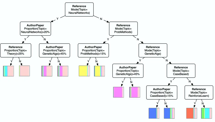
RPTs are selective models that extend classification trees to a relational setting. RPTs also treat het-erogeneous relational subgraphs as a set of attribute multisets, but instead of modeling the multisets as independent values drawn from a multinomial, the RPT algorithm uses aggregation functions to map a set of values into a single feature value. For example, when considering the publication dates on references of a research paper, the RPT could construct a feature that tests whether the average publication date was after 1995. Figure 5 provides an example RPT learned on citation data.

The RPT algorithm automatically constructs and searches over aggregated relational features to model the distribution of the target variable X on items of type t. The algorithm constructs features from the attributes associated with the types TRspecified in the query for t. The algorithm considers

four classes of aggregation functions to group multiset values: mode, count, proportion, and degree (i.e., the number of values in the multiset). For discrete attributes, the algorithm constructs features for all unique values of an attribute. For continuous attributes, the algorithm constructs features for a number of different discretizations, binning the values by frequency (e.g., year>1992). Count, proportion, and degree features consider a number of different thresholds (e.g., proportion(A)>

10%). All experiments reported herein considered 10 thresholds and discretizations per feature.

Reference

A u t horP aper

!"#

Reference

$

%& !'#

A u t horP aper

(

)*+ ,'#

A u t horP aper

$-% $.'#

A u t horP aper

$

( )*+ ,'#

A u t horP aper

$

/0 $.'#

Reference $-% Reference 1 ( )*+ Reference /0 Reference

2$34

5 5 5 5 5

5 5 5

5

5 5

Figure 5: Example RPT to predict machine-learning paper topic.

The RPT algorithm uses recursive greedy partitioning, splitting on the feature that maximizes the correlation between the feature and the class. Feature scores are calculated using the chi-square statistic and the algorithm uses pre-pruning in the form of a p-value cutoff and a depth cutoff to limit tree size and overfitting. All experiments reported herein used p-value cutoff=0.05/|attributes|,

depth cutoff=7. Although the objective function does not optimize pseudolikelihood directly,

prob-ability estimation trees can be used effectively to approximate CPDs consistent with the underlying joint distribution (Heckerman et al., 2000).

The RPT learning algorithm adjusts for biases towards particular features due to degree disparity and autocorrelation in relational data (Jensen and Neville, 2002, 2003). We have shown that RPTs build significantly smaller trees than other conditional models and achieve equivalent, or better, performance (Neville et al., 2003a). These characteristics of RPTs are crucial for learning under-standable RDNs and have a direct impact on inference efficiency because smaller trees limit the size of the final inference graph.

3.4 RDN Inference

The RDN inference graph GIis potentially much larger than the original data graph. To model the

full joint distribution there must be a separate node (and CPD) for each attribute value in GD. To

construct GI, the set of template CPDs in P is rolled out over the test-set data graph. Each

item-attribute pair gets a separate, local copy of the appropriate CPD. Consequently, the total number of nodes in the inference graph will be∑v∈VD|X

T(v)_|+∑

e∈ED|X

T(e)_{|. Roll out facilitates generalization}

across data graphs of varying size—we can learn the CPD templates from one data graph and apply the model to a second data graph with a different number of objects by rolling out more CPD copies. This approach is analogous to other graphical models that tie distributions across the network and roll out copies of model templates (e.g., hidden Markov models, conditional random fields (Lafferty et al., 2001)).

variable is visited (repeatedly) in order, where its value is resampled according to its conditional distribution. Gibbs sampling can be used to extract a unique joint distribution, regardless of the consistency of the model.

Theorem 3 The procedure of a Gibbs sampler applied to an RDN(G,P), where each Xiis discrete and each local distribution in P is positive, defines a Markov chain with a unique stationary joint distribution ˜πfor X that can be reached from any initial state of the chain.

Proof The proof that Gibbs sampling can be used to estimate the joint distribution of a dependency network (Heckerman et al., 2000) applies to rolled out RDNs as well. We restate the proof here for completeness.

Let xt be the sample of x after the tthiteration of the Gibbs sampler. The sequence x1,x2, ...can be viewed as samples drawn from a homogeneous Markov chain with transition matrix ˜P, where

˜

Pi j=p(xt+1= j|xt =i). The matrix ˜P is the product ˜P1·P˜2·...·P˜n, where ˜Pkis the local transition

matrix describing the resampling of Xkaccording to the local distribution of p(xk|pak). The

positiv-ity of the local distributions guarantees the positivpositiv-ity of ˜P. The positivity of ˜P in turn guarantees that the Markov chain is irreducible and aperiodic. Consequently there exists a unique joint distribution that is stationary with respect to ˜P, and this stationary distribution can be reached from any starting point.

This shows that a Gibbs sampling procedure can be used with an RDN to recover samples from a unique stationary distribution ˜π, but how close will this distribution be to the true distribution

π? Small perturbations in the local CPDs could propagate in the Gibbs sampling procedure to pro-duce large deviations in the stationary distribution. Heckerman et al. (2000) provide some initial theoretical analysis that suggests that Markov chains with good convergence properties will be in-sensitive to deviations in the transition matrix. This implies that when Gibbs sampling is effective (i.e., converges), then ˜πwill be close toπand the RDN will be a close approximation to the full joint distribution.

Table 2 outlines the inference algorithm. To estimate a joint distribution, we start by rolling out the model GM onto the target data set GDand forming the inference graph GI. The values of all

unobserved variables are initialized to values drawn from prior distributions, which we estimate em-pirically from the training set. Gibbs sampling then iteratively relabels each unobserved variable by drawing from its local conditional distribution, given the current state of the rest of the graph. After a sufficient number of iterations (burn in), the values will be drawn from a stationary distribution and we can use the samples to estimate probabilities of interest.

For prediction tasks, we are often interested in the marginal probabilities associated with a single variable X (e.g., paper topic). Although Gibbs sampling may be a relatively inefficient approach to estimating the probability associated with a joint assignment of values of X (e.g., when|X|is large), it is often reasonably fast to use Gibbs sampling to estimate the marginal probabilities for each X .

Infer RDN (GD,GM,P,iter,burnin):

GI(VI,EI)←(/0,/0) \\form GI from GDand GM

For each t∈T in GM: For each X_kt∈Xtin GM:

For each vi∈VDs.t.T(vi) =t and ei∈EDs.t.T(ei) =t: VI←VI ∪ {X_ikt}

For each vi∈VDs.t.T(vi) =t and ei∈EDs.t.T(ei) =t:

For each vj∈VDs.t.Xvj ∈paX_ikt and each ej ∈EDs.t.Xej∈paX_ikt:

EI←EI∪ {ei j}

For each v∈VI: \\initialize Gibbs sampling

Randomly initialize xvto value drawn from prior distribution p(xv)

S← /0 \\Gibbs sampling procedure

Choose a random ordering over VI

For i∈iter:

For each v∈VI, in random order:

Resample x0_vfrom p(xv|x− {xv})

xv←x0_v

If i>burnin: S←S∪ {x}:

Use samples S to estimate probabilities of interest

Table 2: RDN inference algorithm.

4. Experiments

The experiments in this section demonstrate the utility of RDNs as a joint model of relational data. First, we use synthetic data to assess the impact of training-set size and autocorrelation on RDN learning and inference, showing that accurate models can be learned with reasonable data set sizes and that the model is robust to varying levels of autocorrelation. In addition, to assess the quality of the RDN approximation for inference, we compare RDNs to RMNs, showing that RDNs achieve equivalent or better performance over a range of data sets. Next, we learn RDNs of five real-world data sets to illustrate the types of domain knowledge that the models discover automatically. In addition, we evaluate RDNs in a prediction context, where only a single attribute is unobserved in the test set, and report significant performance gains compared to two conditional models.

4.1 Synthetic Data Experiments

To explore the effects of training-set size and autocorrelation on RDN learning and inference, we generated homogeneous data graphs with an autocorrelated class label and linkage due to an under-lying (hidden) group structure. Each object has four boolean attributes: X1, X2, X3, and X4. We used

For each object i, 1≤i≤NO:

Choose a group giuniformly from the range[1,NG].

For each object j, 1≤ j≤NO:

For each object k, j<k≤NO:

Choose whether the two objects are linked from p(E|Gj=Gk), a Bernoulli

probability conditioned on whether the two objects are in the same group.

For each object i, 1≤i≤NO:

Randomly initialize the values of X={X1,X2,X3,X4}from a uniform prior dis-tribution.

Update the values of X with 500 iterations of Gibbs sampling using RDN∗, a manually specified model.16

The data generation procedure for X uses a manually specified model where X1 is

autocor-related (through objects one link away), X2 depends on X1, and the other two attribute have no

dependencies. To generate data with autocorrelated X1 values, we used conditional models for p(X1|X1R,X2,X3,X4). RPT0.5 refers to the RPT CPD that is used to generate data with

autocor-relation levels of 0.5. RBC0.5 refers to the analogous RBC CPD. Appendix A contains detailed

specifications of these models. Unless otherwise specified, the experiments use the settings below:

NO = 250,

NG = NO

10,

p(E|Gj=Gk) = {p(E=1|Gj=Gk) =0.50; p(E=1|Gj6=Gk) =

1

NO}, RDN∗ =: [p(X1|X1R,X2,X3,X4) =p(X1|X1R,X2) =RPT0.5or RBC0.5;

p(X2|X1) ={p(X2=1|X1=1) =p(X2=0|X1=0) =0.75};

p(X3=1) =p(X4=1) =0.50].

4.1.1 RDN LEARNING

The first set of synthetic experiments examines the effectiveness of the RDN learning algorithm. We learned CPDs for X1 using the intrinsic attributes of the object(X2,X3,X4)as well as the class

label of directly related objects(X1R). We also learned CPDs for each attribute(X2,X3,X4)using the

class label(X1). This mimics the structure of the true model used for data generation (i.e., RDN∗). We compared two different learned RDNs: RDNRBC uses RBCs for the component learner R; RDNRPT uses RPTs for R. The RPT performs feature selection, which may result in structural inconsistencies in the learned RDN. The RBC does not use feature selection so any deviation from the true model is due to parameter inconsistencies alone. Note that the two models do not consider identical feature spaces so we can only roughly assess the impact of feature selection by comparing

RDNRBCand RDNRPT results.

Theoretical analysis indicates that, in the limit, the true parameters will maximize the pseu-dolikelihood function. This indicates that the pseupseu-dolikelihood function, evaluated at the learned

parameters, will be no greater than the pseudolikelihood of the true model (on average). To evalu-ate the quality of the RDN parameter estimevalu-ates, we calculevalu-ated the pseudolikelihood of the test-set data using both the true models (RDN_RPT∗ , RDN_RBC∗ ) and the learned models (RDNRPT, RDNRBC). If

the pseudolikelihood given the learned parameters approaches the pseudolikelihood given the true parameters, then we can conclude that parameter estimation is successful. We also measured the standard error of the pseudolikelihood estimate for a single test-set using learned models from 10 different training sets. This illustrates the amount of variance due to parameter estimation.

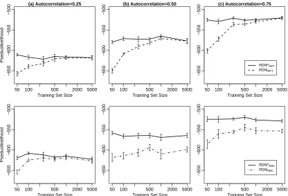
Figure 6 graphs the pseudo-loglikelihood of learned models as a function of training-set size for three levels of autocorrelation. Training-set size was varied at the levels{50,100,250,

500,1000,5000}. We varied p(X1|X1R,X2)to generate data with approximate levels of

autocorre-lation corresponding to{0.25,0.50,0.75}. At each training set size (and autocorrelation level), we generated 10 test sets. For each test set, we generated 10 training sets and learned RDNs. Using each learned model, we measured the pseudolikelihood of the test set (size 250) and averaged the results over the 10 models. We plot the mean pseudolikelihood for both the learned models and the true models. The top row reports experiments with data generated from an RDN_RPT∗ , where we learned an RDNRPT. The bottom row reports experiments with data generated from an RDN_RBC∗ ,

where we learned an RDNRBC.

(a) Autocorrelation=0.25 − 6 5 0 − 6 0 0 − 5 5 0 − 5 0 0

50 100 500 2000 5000

P s e d u o lik e lih o o d

Training Set Size

(b) Autocorrelation=0.50 − 6 5 0 − 6 0 0 − 5 5 0 − 5 0 0

50 100 500 2000 5000

Training Set Size

(c) Autocorrelation=0.75 − 6 5 0 − 6 0 0 − 5 5 0 − 5 0 0

50 100 500 2000 5000

Training Set Size RDN*RPT RDNRPT − 6 5 0 − 6 0 0 − 5 5 0 − 5 0 0

50 100 500 2000 5000

P s e d u o lik e lih o o d

Training Set Size

− 6 5 0 − 6 0 0 − 5 5 0 − 5 0 0

50 100 500 2000 5000

Training Set Size

− 6 5 0 − 6 0 0 − 5 5 0 − 5 0 0

50 100 500 2000 5000

Training Set Size RDN*RBC RDNRBC

Figure 6: Evaluation of RDN learning.

These experiments show that the learned RDNRPT is a good approximation to the true model by

There appears to be little difference between the RDNRPT and RDNRBCwhen autocorrelation is

low, but otherwise the RDNRBCneeds significantly more data to estimate the parameters accurately.

One possible source of error is variance due to lack of selectivity in the RDNRBC, which necessitates

the estimation of a greater number of parameters. However, there is little improvement even when we increase the size of the training sets to 10,000 objects. Furthermore, the discrepancy between the estimated model and the true model is greatest when autocorrelation is moderate. This indicates that the inaccuracies may be due to the naive Bayes independence assumption and its tendency to produce biased probability estimates (Zadrozny and Elkan, 2001).

4.1.2 RDN INFERENCE

The second set of synthetic experiments evaluates the RDN inference procedure in a prediction context, where only a single attribute is unobserved in the test set. We generated data with the

RDN_RPT∗ and RDN_RBC∗ as described above and learned models for X1 using the intrinsic attributes

of the object (X2,X3,X4) as well as the class label and the attributes of directly related objects

(X1R,X2R,X3R,X4R). At each autocorrelation level, we generated 10 training sets (size 500) to learn

the models. For each training set, we generated 10 test sets (size 250) and used the learned models to infer marginal probabilities for X1on the test set instances. To evaluate the predictions, we report

area under the ROC curve (AUC).17 These experiments used the same levels of autocorrelation outlined above.

We compare the performance of four types of models. First, we measure the performance of RPTs and RBCs. These are conditional models that reason about each instance independently and do not use the class labels of related instances. Second, we measure the performance of learned RDNs: RDNRBCand RDNRPT. For RDN inference, we used fixed-length Gibbs chains of 2000

sam-ples with burn-in of 100. Third, we measure performance of the learned RDNs while allowing the true labels of related instances to be used during inference. This demonstrates the level of perfor-mance possible if the RDNs could infer the true labels of related instances with perfect accuracy. We refer to these as ceiling models: RDN_RBCceil and RDN_RPTceil. Fourth, we measure the performance of two RMNs described below.

The first RMN is non-selective. We construct features from all the attributes available to the RDNs, defining clique templates for each pairwise combination of class label value and attribute value. More specifically, the available attributes consist of the intrinsic attributes of objects, and both the class label and attributes of directly related objects. The second RMN, which we refer to as RMNSel, is a hybrid selective model—clique templates are only specified for the set of attributes

selected by the RDN during learning. For both models, we used maximum-a-posteriori parameter estimation to estimate the feature weights, using conjugate gradient with zero-mean Gaussian priors, and a uniform prior variance of 5.18For RMN inference, we used loopy belief propagation (Murphy et al., 1999).

We do not compare directly to RBNs because their acyclicity constraint prevents them from representing the autocorrelation dependencies in this domain. Instead, we include the performance of conditional models, which also cannot represent the autocorrelation of X1. Although RBNs and

conditional models cannot represent the autocorrelation directly, they can exploit the autocorre-lation indirectly by using the observed attributes of related instances. For example, if there is a

17. Squared-loss results are qualitatively similar to the AUC results reported in Figure 7.

correlation between the words on a webpage and its topic, and the topics of hyperlinked pages are autocorrelated, then the models can exploit autocorrelation dependencies by modeling the contents of a webpage’s neighboring pages. Recent work has shown that collective models (e.g., RDNs) are a low-variance means of reducing bias through direct modeling of the autocorrelation dependen-cies (Jensen et al., 2004). Models that exploit autocorrelation dependendependen-cies indirectly by modeling the observed attributes of related instances, experience a dramatic increase in variance as the number of observed attributes increases.

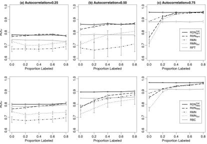
During inference we varied the number of known class labels in the test set, measuring perfor-mance on the remaining unlabeled instances. This serves to illustrate model perforperfor-mance as the amount of information seeding the inference process increases. We expect performance to be sim-ilar when other information seeds the inference process—for example, when some labels can be inferred from intrinsic attributes, or when weak predictions about many related instances serve to constrain the system. Figure 7 graphs AUC results for each model as the proportion of known class labels is varied.

Figure 7: Evaluation of RDN inference.

The data for the first set of experiments (top row) were generated with an RDN_RPT∗ . In all configurations, RDNRPT performance is equivalent, or better than, RPT performance. This indicates

that even modest levels of autocorrelation can be exploited to improve predictions using an RDNRPT. RDNRPT performance is indistinguishable from that of RDNRPTceil except when autocorrelation is high

and there are no labels to seed inference. In this situation, the predictive attribute values (i.e., X2) are

exploit the autocorrelation dependencies. When there is no information to anchor the predictions, there is an identifiability problem—symmetric labelings that are highly autocorrelated, but with opposite values, appear equally likely. In situations where there is little seed information (either attributes or class labels), identifiability problems can increase variance and bias RDN performance towards random.

When there is low or moderate autocorrelation, RDNRPT performance is significantly higher

than both RMNs. In these situations, poor RMN performance is likely due to a mismatch in feature space with the data generation model—if the RMN features cannot represent the data dependencies that are generated with aggregated features, the inferred probabilities will be biased. When there is high autocorrelation, RDNRPT performance is indistinguishable from RMN, except when there

are no labels to seed inference—the same situation where RDNRPT fails to meet its ceiling. When

autocorrelation is high, the mismatch in feature space is not a problem. In this situation most neighbors share similar attribute values, thus the RMN features are able to accurately capture the data dependencies.

The data for the second set of experiments (bottom row) were generated with an RDN_RBC∗ . The

RDNRBCfeature space is roughly comparable to the RMN because the RDNRBCuses multinomials to

model individual neighbor attribute values. On these data, RDNRBCperformance is superior to RMN

performance only when there is low autocorrelation. RMNSel uses fewer features than RMN and it

has superior performance on the data with low autocorrelation, indicating that the RMN learning algorithm may be overfitting the feature weights and producing biased probability estimates. We experimented with a range of priors to limit the impact of weight overfitting, but the effect remained consistent.

RDNRBCperformance is superior to RBC performance only when there is moderate to high

au-tocorrelation and sufficient seed information. When auau-tocorrelation is low, the RBC is comparable to both the RDN_RBCceil and the RDNRBC. Even when autocorrelation is moderate or high, RBC

perfor-mance is still relatively high. Since the RBC is low-variance and there are only four attributes in our data sets, it is not surprising that the RBC is able to exploit autocorrelation to improve performance. What is more surprising is that RDNRBCrequires substantially more seed information than RDNRPT

in order to reach ceiling performance. This indicates that our choice of model should take test-set characteristics (e.g., number of known labels) into consideration.

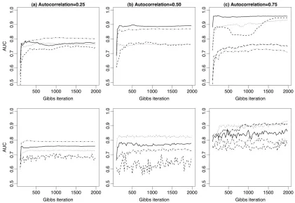
To investigate Gibbs sampling convergence, we tracked AUC throughout the RDN Gibbs sam-pling procedure. Figure 8 demonstrates AUC convergence on each inference task described above. We selected a single learned model at random from each task and report convergence from the trials corresponding to five different test sets. AUC improves very quickly, often leveling off within the first 250 iterations. This shows that the approximate inference techniques employed by the RDN may be quite efficient to use in practice. However, when autocorrelation is high, longer chains may be necessary to ensure convergence. There are only two chains that show a substantial increase in performance after 500 iterations and both occur in highly autocorrelated data sets. Also, the

RDNRBC chains exhibit significantly more variance than the RDNRPT chains, particularly when