CarpeDiem: Optimizing the Viterbi Algorithm and
Applications to Supervised Sequential Learning
Roberto Esposito [email protected]
Daniele P. Radicioni [email protected]
Department of Computer Science University of Turin
Corso Svizzera, 185 - 10149 Turin - Italy
Editor: Michael Collins
Abstract
The growth of information available to learning systems and the increasing complexity of learn-ing tasks determine the need for devislearn-ing algorithms that scale well with respect to all learnlearn-ing parameters. In the context of supervised sequential learning, the Viterbi algorithm plays a funda-mental role, by allowing the evaluation of the best (most probable) sequence of labels with a time complexity linear in the number of time events, and quadratic in the number of labels.
In this paper we propose CarpeDiem, a novel algorithm allowing the evaluation of the best possible sequence of labels with a sub-quadratic time complexity.1We provide theoretical ground-ing together with solid empirical results supportground-ing two chief facts. CarpeDiemalways finds the optimal solution requiring, in most cases, only a small fraction of the time taken by the Viterbi algorithm; meantime,CarpeDiemis never asymptotically worse than the Viterbi algorithm, thus confirming it as a sound replacement.
Keywords: Viterbi algorithm, sequence labeling, conditional models, classifiers optimization, exact inference
1. Introduction
In supervised learning systems, classifiers are learnt from sets of labeled examples and then used to predict the “correct” labeling for new objects. According to how relations between objects are exploited to build and evaluate the classifier, different categories of learning systems can be individ-uated. When the learning system deals with examples as isolated individuals, thus disregarding any relation among them, the system is said to work in a propositional setting. In this case classifiers can optimize the assignment of labels individually. Instead, in the setting of supervised sequential learning (SSL) the objects are assumed to be arranged in a sequence: relationships between previous and subsequent objects exist, and are used to improve the classification accuracy. SSL classifiers are then required to find the globally optimum sequence of labels, rather than the sequence of locally optimal labels. For instance, in the optical character recognition task, the labelling “learning” is probably better than “learn1ng”, even though the description of the sixth character taken in isola-tion might suggest otherwise. A SSL classifier may deal with such ambiguities by exploiting the
1. The implementation ofCarpeDiemand of several sequence learning algorithms can be downloaded at: http://www.di.unito.it/˜esposito/Software/seqlearning.tar.gz
a working GUI (Mac OS X only) for experimenting with the software can be downloaded at:
higher sequential correlation, in the English language, of the bigram in with respect to 1n. Concep-tually, given a sequence of T observations and K possible labels, KTpossible combinations of labels are to be considered by SSL classifiers. Most systems deal with such complexity by assuming that relations may span only over nearby objects and use the Viterbi algorithm (Viterbi, 1967) to find the globally optimal sequence of labels inΘ(T K2)time.
In the last few years it has become increasingly important for supervised sequential learning algorithms to handle problems with large state spaces (Dietterich et al., 2008). Unfortunately, even the drastic reduction in complexity achieved by the Viterbi algorithm may be not sufficient in such domains. For instance, this is the case of web-logs related tasks (Felzenszwalb et al., 2003), music analysis (Radicioni and Esposito, 2007), and activity monitoring through body sensors (Siddiqi and Moore, 2005), where the number of possible labels is so large that the classification time can grow prohibitively high.
Some recent works propose techniques that under precise assumptions allow faster execution time of classifiers based on hidden Markov models (HMMs) (Rabiner, 1989). One feature shared by these approaches is the assumption that the transition matrix has a specific form allowing one to rule out most transitions. Such approaches are highly valuable when the problem naturally fits the assumption; vice versa they either lose the optimal solution or cannot be applied at all, when it does not. Moreover, they assume the transition matrix to be known beforehand and fixed over time. While this is a natural assumption in HMMs, recent algorithms based on the boolean features framework (McCallum et al., 2000) allow for more general settings where the transition matrix is itself a function of the observations around the object to be labelled. In such cases it is hard to figure out how the aforementioned approaches apply.
In this paper we introduce CarpeDiem. It is a parameter-free algorithm, sporting best case sub-quadratic complexity, devised as a replacement for the Viterbi algorithm. CarpeDiem avoids considering a transition whenever local observations make it impossible for the transition to be part of the optimal path. CarpeDiempreserves the optimality of the result, never being asymptotically worse than the Viterbi algorithm. Moreover,CarpeDiemautomatically adapts to the sequence being evaluated, so that its complexity degrades to the Viterbi algorithm complexity in case the underlying assumption is not met. Interestingly, in contrast with alternative approaches, the assumption made byCarpeDiemneeds not be “always” valid. On the contrary, the algorithm is able to take advantage of the assumption even when it holds for small portions of the sequence. This implies that the worst case complexity is hit only in the very unlikely situation where the assumption does not hold for the entire sequence. Finally,CarpeDiemcan be directly applied in any sequential learning system based on the Viterbi algorithm, even in those where the transition matrix changes over time.
The present work is structured as follows: we briefly recall the Viterbi algorithm and state the problem (Section 2). After surveying related work (Section 3), we illustrate CarpeDiem in full detail, and an execution example on a toy problem is provided (Section 4). We then show how
2. Preliminaries
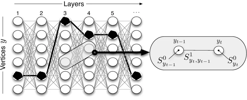
The problem of finding the best sequence of labels is often represented as a search for the optimal path in a layered and weighted graph (Figure 1).
Definition 1 Layered graph. A layered graph is a connected graph where vertices are partitioned into a set of “layers” such that: i) edges connect only vertices in adjacent layers; ii) any vertex in a given layer is connected to all vertices of the successive layer.
We adopt the convention of indicating the layer to which a vertex belongs as a subscript to the vertex name, so that yt denotes a vertex in layer t. We associate to each vertex yt a weight S0yt, and to each edge(yt−1,yt) a weight S1yt,yt−1 (Figure 1). In the following we use the term “vertical” in referring to “per node” properties. For instance, we will use the expressions “vertical weight” of yt and “vertical information” to refer to S0yt and to the information provided by evidence related to
vertices, respectively. Similarly, we use the term “horizontal” in referring to “per edge” properties. For instance, we will use the expression “horizontal weight” in referring to the weight associated to a given transition. The distinction between vertical and horizontal information is important in the present work, the key idea inCarpeDiemis to exploit vertical information to avoid considering the horizontal one.
Given a layered and weighted graph with T layers and K vertices per layer, a path is a sequence of vertices y1,y2, . . . ,yt (1≤t≤T ). The reward for a path is the sum of the vertical and horizontal weights associated to the path:
reward(y1,y2, . . . ,yt) = t−1
∑
u=1
S0yu+S1yu+1,yu !
+S0yt.
We defineγ(yt)as the maximal reward associated to any path from any node in layer 1 to yt:
γ(yt) = max
y1,y2,...,yt−1
reward(y1,y2, . . . ,yt−1,yt).
We consider the problem of picking the maximal path from the leftmost layer to the rightmost layer. The naive solution considers all the KT possible paths, and returns the maximal one. The Viterbi algorithm (Viterbi, 1967) solves the problem inΘ(T K2)time by exploiting a dynamic pro-gramming strategy. The main idea stems from noticing that the reward of the best path to node yt can be recursively computed as: i) the reward of the best path to the predecessorπ(yt)on the optimal path to yt; ii) plus the reward for transition S1y
t,π(yt); iii) plus the weight of node yt. In formulae:
γ(yt) =
(
S0yt if t=1
γ(π(yt)) +S1y
t,π(yt)+S
0
yt otherwise.
(1)
We will also make use of the equivalent formulation obtained by noticing that π(yt) is the best predecessor for yt. That is, π(yt) is the vertex yt−1 (in layer t−1) that maximizes the quantity
γ(yt−1) +S1yt,yt−1. Then:
γ(yt) =
( S0
yt if t=1
maxyt−1 γ(yt−1) +S
1
yt,yt−1+S
0
yt
Figure 1: S0yt and S0yt−1 denote per vertex (vertical) weights. S1yt,yt−1 denotes per edge (horizontal) weights.
The Viterbi algorithm proceeds from left to right storing the values ofγinto an arrayGas soon as
such values are computed. Assuming that∀yt−1:G(yt−1) =γ(yt−1), thenG(yt)is computed as:
G(yt) =max
yt−1
G(yt−1) +S1y
t,yt−1+S
0
yt
.
The pseudo code for the algorithm is reported in Algorithm 1. Since the maximization at the line marked with label number 1 (henceforth simply “line 1 ”) requiresΘ(K)time, the time needed for processing each layer is in the order ofΘ(K2). The total time required by Viterbi is thenΘ(K2T). The standard formulation of the Viterbi algorithm would also store the optimal path information as it becomes available. Since this can be done using standard techniques (Cormen et al., 1990, page 520) without affecting the complexity of the algorithm, we do not explicitly report that in the pseudo-code.
Let us now consider how the above definitions instantiate in the context of a learning environ-ment. The symbol S0yt conveys information about label yt provided by observing the data at time t. In hidden Markov models terminology, S0yt corresponds to probability byt(xt)of observing symbol
xt in state yt (Rabiner, 1989, definition of bj(k)pag. 261, Eq. 8). More generally, S0yt is a quantity
that depends on both the label yt predicted for time (layer) t and the observations at and around time t. Likewise, in HMMs terminology, Sy1′,y corresponds to the probability ayy′ of transiting from state
y to state y′ (Rabiner, 1989, definition of ai j pag. 260, Eq. 7). More in general, S1y′,y may depend
on both the labels(y′,y)and on the observations at and around the current layer. We note that since S1y′,y may vary over time (which motivates the notation S1yt,yt−1), the setup considered here is more
begin
forall y1do G(y1)←S0
y1;
end
for t=2 to T do
forall ytdo
1 G(yt)←maxyt−1 G(yt−1) +S
1
yt,yt−1+S
0
yt
;
end end
y∗T←arg maxyTG(yT);
return y∗T;
end
Algorithm 1: The Viterbi algorithm.
3. Related Work
As we illustrated in Section 1, in cases where hundreds or thousands of labels are to be handled, the quadratic dependence on the number of labels is still a high burden that limits the applicability of sequential learning techniques.
In other fields (e.g., telecommunications) there exist ad hoc solutions that allow one to tame the complexity of the Viterbi algorithm by means of hardware implementations (Austin et al., 1990) or methods for approximating the optimum path (Fano, 1963). For instance, in the research field of speech recognition, the Viterbi algorithm is routinely applied to huge problems. This is a typical case where approximate solutions really pay off: suboptimal paths could be tolerated (to some ex-tent) and tight time constraints prevent exhaustive search. A popular approach in this field is the Viterbi beam search (VBS) (Lowerre and Reddy, 1980; Spohrer et al., 1980; Bridle et al., 1982): essentially, VBS performs a breadth-first suboptimal search in which only the most promising solu-tions are retained at each step. Many improvements over this basic strategy have been proposed to refine either the computational performance or the accuracy of the solution (e.g., Ney et al., 1992). In most cases domain-based knowledge (such as language constraints) is used to restrict the search efforts to some relevant regions of the search space (Ney et al., 1987). Also, in recent years, several algorithms have been proposed that overcome the difficulties inherent in heuristic ranking strategies by learning ranking functions specifically optimized for the problem at hand (Xu and Fern, 2007).
has two drawbacks: at learning time, it hinders the process of finding better classifiers (or at least it slows the process down); at testing time, it yields sub-optimal classifications.
In recent years, despite a widespread usage of the Viterbi algorithm within the sequential learn-ing field, only few works addressed the problem of reduclearn-ing its time complexity and at the same time retaining the optimal result. In Felzenszwalb et al. (2003), linear (and near linear) algorithms are proposed to compute the optimal labels sequence. Their algorithms work under the assumption that the reward for the transition between states number i and j is a “simple” function of|i−j|.2
In Siddiqi and Moore (2005) it is assumed that the transition matrix is well approximated by a particular one where, for each vertex, the probability mass is concentrated on the k highest transi-tions leaving it. Then, the weights associated to the other transitransi-tions are approximated by a constant, and the optimal path is evaluated withΘ(kKT)time complexity. Clearly, the smaller k, the faster the algorithm.
Both techniques provide significant time savings with respect to the Viterbi algorithm. However, they are both based on assumptions about the entries in the transition matrix that are not guaranteed to hold in practice. More in particular, the assumption by Felzenszwalb et al. (2003) does not seem to easily fit general cases. Also, the investigation needed to devise the correct parameter space may require knowledge and efforts that are not always at disposal of the average practitioner. The as-sumption underlying the work of Siddiqi and Moore (2005) is, in our opinion, simpler to be fulfilled in practice. However, the extent to which it holds (which determines the magnitude of k) cannot be easily forecasted. Again, the extra efforts needed to assess the applicability of the approach may be detrimental to its application. Moreover, both approaches require homogeneous transition matrices: that is, transition matrices that do not vary over time. This is a common assumption, but unfortunately it cannot be guaranteed in some recently developed approaches, as those based on the boolean feature framework (McCallum et al., 2000). CarpeDiemcan be safely applied even in this more complex scenario. In the experimentation, we successfully applyCarpeDiemin both settings, the one where the transition matrix is not constant (Section 6.1), as well as the one where it is (Sections 6.2 and 6.3).
In a recent paper Mozes et al. (2007) propose an exact compression-based technique to speed up the Viterbi algorithm. The authors propose to use three well known compression schemes achiev-ing significant speed-ups whose magnitude depends on which compression algorithm is adopted. Interestingly the cited approach is not a search scheme, rather it is a preprocessing step. As such, it qualifies as an orthogonal technique amenable to be used together withCarpeDiemobtaining the advantages of both techniques.
In facts, to the best of our knowledge, the algorithmsCarpeDiemand (Mozes et al., 2007) are the only exact ones, capable of speeding up the Viterbi algorithm when the assumption of homo-geneous matrices is dropped. We would also argue that the other approaches presented above are not easily adapted to work in this, more complex, scenario. In Siddiqi and Moore (2005) the tran-sition matrix needs to be traversed in advance in order to obtain the highest ranking frequencies. If those frequencies change over time, this operation needs to be repeated for each t, and the algorithm would require O(T K2)only to compute this preprocessing step. In Felzenszwalb et al. (2003) it is necessary to express the weights of the transition from label i to label j in terms of a function of
|i−j|. The effectiveness of the approach depends on particular properties of this function. It could be argued that, in very particular situations, those properties could be shown to hold even when
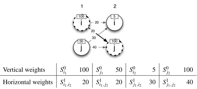
Vertical weights S0
i1 100 S0j1 50 S0i2 5 S0j2 100
Horizontal weights S1i1,i2 20 Si11,j2 20 S1j1,i2 30 S1j1,j2 40
Figure 2: Sometimes horizontal weights can be disregarded without loosing the optimal path.
the transition matrix varies with t. However, it is hard to figure out a general way to enforce this property without inspecting the whole transition matrix at each time step.
CarpeDiemenjoys the desirable property of smoothly scaling to the Viterbi algorithm complex-ity when the underlying assumptions soften (as argued in Section 4.5). This has two consequences: 1) the algorithm adapts to the problem and to the sequence at hand, and 2) the algorithm can be uni-versally applied (even when one is unsure about whether the problem fitsCarpeDiemassumptions or not). In contrast with other state-of-the-art algorithms, no domain knowledge is to be given, nor any parameter needs to be set. This makesCarpeDiemwell suited to be used on a regular basis as a drop-in replacement of the Viterbi algorithm: in the worst case, with no time saving.
4. TheCarpeDiemAlgorithm
In the general case, in order to determine the end point of the best path to a given layer, one can avoid inspecting all vertices in that layer. In particular, after sorting the vertices in layer t according to their vertical weight, the search can be stopped when the difference in vertical weight of the best node so far and the next vertex in the ordering is big enough to counterbalance any advantage that can be possibly derived from exploiting a better transition and/or a better ancestor.
To clarify this point, it is interesting to consider the minimal example reported in Figure 2. Let us assume that the reward for the maximal weight for any transition is 60. Our objective is to find the endpoint of the best path to each layer. For layer 1 we have no incoming paths, the best endpoint is simply the vertex with the maximal vertical weight: in the example, i1. In our approach, we consider
vertices with highest vertical weight first. Hence we start by calculating the reward of the optimal path to node j2: in the example, the path i1,j2(with score S0i1+S1j2,i1+S0j2 =100+20+100=220). We notice that the reward attainable by reaching i2cannot be higher than 165, computed as the sum
of the reward for the best path to layer 1 (i.e., 100), plus the maximal weight for any transition (i.e., 60), plus the vertical weight of i2 (i.e., 5). Therefore the endpoint of the best path to layer
2 must be j2 and it is not necessary to calculate the reward for reaching i2. In the course of the
each layer (Algorithm 3), and one that finds the reward for reaching a given node by traversing the graph from right to left (Algorithm 4).
We say that a vertex is open if the reward of its best incoming path has been computed; otherwise the vertex is said to be closed.CarpeDiemfinds the best vertex for each layer by calling Algorithm 3 (also referred to as forward search strategy), which leaves closed as many vertices as possible. The backward search strategy is called to open vertices whenever necessary.
The main procedure ofCarpeDiemis presented in Algorithm 2; the forward and the backward search strategies are presented in Algorithms 3 and 4, respectively. Before detailing the algorithm, we need to introduce several definitions.
Definition 2 Let us define:
S1∗ : an upper bound to the maximal transition weight in the current graph S1∗≥ max
yt,yt−1
S1yt,yt−1; (3)
γ∗
t : the reward of the best path to any vertex in layer t (including the vertical weight of the ending vertex)
γ∗
t =maxy
t
γ(yt);
βt : an upper bound to the reward that can be obtained in reaching layer t (2≤t≤T )
βt=γ∗t−1+S1∗; (4)
⊒t : a total ordering—based on vertical weights—of vertices at layer t.
⊒t≡ {(yt,yt′)|S0yt >S
0
y′t}. (5)
Also, we say that vertex yt is more promising than vertex y′t iff yt ⊒tyt′.
During execution, CarpeDiem calculates several values that are strictly connected to the def-initions above. In particular Gis a vector of K×T elements. G(yt) contains the value of γ(yt)
as calculated by CarpeDiem. Also, Bis a vector of T elements. Bt contains the value of βt as
calculated byCarpeDiem. To a good extent, provingCarpeDiemcorrect will involve proving that, indeed,G(yt) =γ(yt)andBt=βt.
4.1 Algorithm 2 – Main Procedure
Algorithm 2 initializesG(y1)andB2values and calls Algorithm 3 on all layers 2. . .T . More
specif-ically,G(y1)is set to S0
1(as required by Equation 1). AlsoB2is set to the maximal vertical weight
found plus S1∗(as required by Equation 4).
4.2 Algorithm 3 – Forward search strategy
The forward strategy searches for the best vertex for layer t stopping as soon as this vertex can be determined unambiguously.
begin
foreach y1{Initialization Step}do 2 G(y1)←S0y1;{Opens vertex y1}
end
3 y∗1←arg maxy1(G(y1)); B2←G(y∗
1) +S1∗;
foreach layer t∈2. . .T do
y∗t ←result of Algorithm 3 on layer t;
end
return path to y∗T;
end
Algorithm 2:CarpeDiem.
begin
y∗t ←most promising vertex; y′t←next vertex in the⊒t ordering; Open vertex y∗t {call Algorithm 4};
whileG(y∗
t)<Bt+S0y′
t do
4 Open vertex y′t {call Algorithm 4}; 5 y∗t ←arg maxy′′∈{y∗
t,y′t}[G(y
′′)];
y′t←next vertex in the⊒t ordering;
end
6 Bt+1←G(y∗t) +S1∗; return y∗t;
end
Algorithm 3: Forward search strategy.
case, the algorithm can avoid opening all vertices in every layer. The search is stopped when the difference in vertical weight of y∗t and y′t is big enough to counterbalance any advantage that can be possibly derived from exploiting a better transition and/or a better ancestor. In formulae, letπ(y∗t)
be the best predecessor for y∗t, the (forward) search is stopped when the currently best vertex yt∗and the next vertex y′t in the⊒t ordering satisfy:
accounts for a better vertical weight of y∗t w.r.t. yt
z }| {
Sy0∗
t −S
0
yt′ ≥
accounts for a possibly bet-ter predecessor of y′tw.r.t. y∗t
z }| {
γ∗
t−1−γ(π(y∗t)
+
accounts for a possibly bet-ter transition from y′t
prede-cessor
z }| {
S1∗−S1y∗
t,π(y∗t)
. (6)
The above formula is a direct consequence of the exit condition of the while loop of Algorithm 3, and it can be obtained by substituting3BandGwithβandγ, and then expandingβandγusing their
definitions (we repeat the relevant definitions in Table 1-a and b).
a) Definition ofβ βt =γ∗t−1+S1∗
b) Definition ofγ(see Eq. 1) γ(y∗t) =γ(π(yt∗)) +S1y∗
t,π(y∗t)+S
0
y∗t
Table 1: Summary of few useful quantities
In case the stop criterion is not met, the algorithm calls Algorithm 4 (also referred to as the backward strategy) which setsG(y′t) =γ(y′t). If necessary, the “maximal” vertex y∗t (the vertex that,
so far, has associated maximal reward) is updated. Before exiting,Bt+1is readied for later use, and
the best vertex is returned.
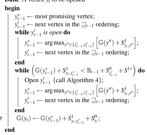
4.3 Algorithm 4 – Backward search strategy
The backward search strategy opens a vertex yt by finding its best ancestor and settingG(yt) accord-ingly. In much the same spirit as in the forward strategy, the algorithm saves some computation i) by exploiting⊒t−1in order to inspect first the most promising vertices, and ii) by taking advantage
ofβt−1in order to stop the search as soon as possible.
Data: A vertex yt to be opened
begin
y∗t−1←most promising vertex;
y′t−1←next vertex in the⊒t−1ordering; while y′t−1is open do
y∗t−1←arg maxy′′∈{y′
t−1,y∗t−1}
h
G(y′′) +S1
yt,y′′
i
;
y′t−1←next vertex in the⊒t−1ordering; end
while
G(y∗
t−1) +S1yt,y∗t−1 <
Bt−1+S0
yt′−1+S
1∗do
Open y′t−1{call Algorithm 4};
y∗t−1←arg maxy′′∈{y′
t−1,y∗t−1}
h
G(y′′) +S1
yt,y′′
i
;
y′t−1←next vertex in the⊒t−1ordering; end
7 G(yt)←G(y∗t−1) +S1yt,y∗t−1+S
0
yt;
end
Algorithm 4: Backward search strategy to open yt.
The first loop finds the best predecessor among the open vertices of layer t−1. In the second loop, we exploit the same idea behind the forward strategy. Let us inspect the exit condition of the second loop:
G(y∗t
−1) +S1yt,y∗t−1<
Bt−1+S0
y′
t−1+S
1∗.
With the exception of the symbols in bold font, the formula is the same as the one in the exit condition of the while loop in Algorithm 3. The bold symbols take into account the transition to the target vertex. Namely, S1y
t,y∗t−1 takes into account the transition from the current best vertex (y ∗
to the target vertex yt and S1∗accounts for the maximal reward that a transition from y′t−1to yt can possibly obtain.
Also the internal working of the second loop is very similar to the one in the forward strategy. After opening (through a recursive call) y′t−1, the current best vertex is set to the best of y′t−1and y∗t−1.
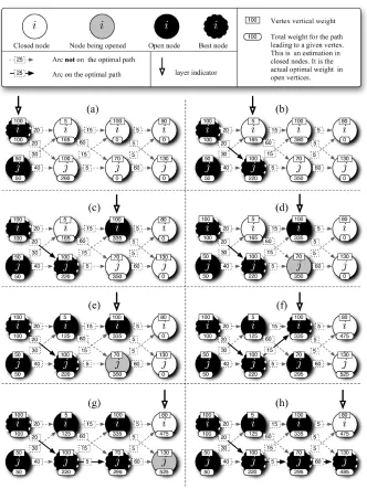
4.4 Example
In the following we provide a description of an execution ofCarpeDiemover a toy problem. The problem consists of labeling a sequence containing four events and two labels (named i and j). The example is reported in Figure 3. The weight shown on the edge between labels yt−1 and yt
corre-sponds to S1yt,yt−1. The bound S1∗ on the maximum horizontal reward is 60. Two further quantities are reported in the figure, and shown graphically by means of boxes placed on vertices: within rectangular boxes, we report the vertical weight of the vertex. Within rounded boxes, we report:
• G(yt), if yt is open;
• Bt+S0
yt, if yt is closed andBt has already been computed;
• 0, otherwise.
Here we give a detailed description of the algorithm execution over the given graph.
step (a) At the beginning of the execution, all vertices are closed. The initialization steps in
Algo-rithm 2 open all vertices in layer 1. Clearly, there is no reward for arriving at vertices in layer 0 and no incoming transitions to be taken into account. The best vertex in layer 1 is thus the vertex having the maximum vertical weight.
step (b) The analysis of layer 2 starts by opening the most promising vertex in that layer (vertex j).
Since all vertices at layer 1 are open, the backward strategy already has complete information at disposal, and it does not need to enter the second loop to open j2. OnceG(j2)has been
computed, the algorithm compares this value to the bound on the weight of the best path to i2. Since S0i2+B2=165 cannot outperformG(j2) =220, there is no need to open vertex i2. step (c) To open i3, the backward strategy goes back to layer 2 and searches for the best path to
that vertex. Again, vertex i2can be left closed, since there is no chance that the best path to i3
traverses it. In fact,
B2+S0
i2+S1∗= (100+60) +5+60=225 cannot outperform the reward
G(j2) +S1
i3,j2 =220+15=235
obtained by passing through j2. ThenG(i3)is set to 235+100=335.
Unfortunately, this does not allow to make a definitive decision about whether this is the best vertex of layer 3, sinceB3+S0
Figure 3:CarpeDiemin action on a toy problem.
step (d) The goal is, at this point, to find the best path to j3. Even though j2has a clear advantage
over i2, this does not suffice to exclude that the latter one is on the optimal path to j3(since G(j2) +S1
j3,j2 6<B2+S0i2+S1∗): the backward strategy is then forced to recursively call itself to open i2.
step (e) By opening i2, the algorithm setsG(i2)to 125 (the best path being i1→i2), thus ruling it
out as a candidate for being on the optimal path to j3.
step (f) In returning to consider layer 3, we are back to the path i1→ j2→i3. To open vertices i2
step (g) The first vertex to be opened in its layer is j4. Interestingly, the best path to j4 is not
through the best vertex in layer 3. In fact, while the highest reward for a three steps walk is on vertex i3, it is more convenient to go through vertex j3to reach vertex j4.
step (h) SinceG(j4) =485 is larger thanB4+S0
i4, the algorithm terminates leaving i4closed. In Section 6 real world problems are considered, and much larger optimizations obtained.
4.5 Algorithm Properties
An intuitive way of characterizing the algorithm complexity is to consider Formula 6, where the exit condition of Algorithm 3 is rewritten in order to point out why in some cases it is safe to stop inspecting the current layer. Clearly, the sooner the loop exit condition is satisfied, the faster the algorithm.
Arguably, the worst case happens when vertical rewards, being equal for each label, do not provide any discriminative power. In such a case, the left term in Formula 6 is zero, the inequality is never satisfied, and Algorithm 3 calls Algorithm 4 over all K vertices in every layer. In this case, for each one of the k vertices to be opened in a new layer, the first loop of Algorithm 4 iterates over all K predecessors. However, no recursive call takes place. Overall, in the worst case hypothesis,
CarpeDiemhas order of O(T KK+T K log(K)) =O(T K2)time complexity.4 CarpeDiemis never asymptotically worse than the Viterbi algorithm.
The best case happens when horizontal rewards, being equal for each transition, do not provide any discriminative power. In such a case the right hand side of the inequality in Formula 6 is zero and the inequality is guaranteed to be satisfied immediately. Moreover, being the backward strategy based on a bound similar to the one that leads to Formula 6, it will never open any other vertex. Then, a single vertex per layer is opened andCarpeDiemhas order of O(T+T K log(K)) =O(T K log(K))
time complexity. A more formal argument aboutCarpeDiem complexity is stated by Theorem 3 and proved in Appendix B.
Theorem 3 CarpeDiem has O(T K2)worst case time complexity and O(T K log K)best case time complexity.
CarpeDiemfinds the optimal sequence of labels. By using standard book-keeping techniques, the optimal sequence of labels can be tracked back by starting from the optimal end point. Then, the optimality ofCarpeDiemcan be proved by showing that the vertex returned by the forward strategy at the end of the algorithm is the end-point of the optimal path through the graph. This property, stated by Theorem 1, is formally proved in Appendix A.
Theorem 1 Let us consider a sequence of calls to Algorithm 3 on layers 2,3, . . . ,t(t≤T). When Algorithm 3 terminates on layer t, the returned vertex y∗t is the endpoint of the optimal path to layer t. Formally,
∀yt :γ(yt∗)≥γ(yt).
Beside the theoretical properties of the algorithm, it is important for the practitioner to consider its actual performances over real world problems. In the general case the algorithm will open some, but not all vertices: the exact number of the vertices that will be inspected depends on the particular
application and on how the features have been engineered. Empirical evidence (Section 6) suggests that many problems are closer to the best case than to the worst. Before introducing the experi-mentation, we show howCarpeDiemcan be instantiated in the context of a supervised sequential learning system and, more in particular, in a system based on the voted perceptron algorithm.
5. Grounding the Voted Perceptron Algorithm onCarpeDiem
The supervised sequential learning problem can be formulated as follows (Dietterich, 2002).
Let{(~xi,~yi)}Ni=1 be a set of N training examples. Each example is a pair of sequences (~xi,~yi), where~xi=hxi,1,xi,2, . . . ,xi,Tii and~yi=hyi,1,yi,2, . . . ,yi,Tii. The goal is to
con-struct a classifier H that can correctly predict a new label sequence~y=H(~x)given an input sequence~x.
The SSL problem has been approached with many different techniques. Among others, we recall Sliding Windows (Dietterich, 2002), hidden Markov models (Rabiner, 1989), Maximum Entropy Markov Models (McCallum et al., 2000), Conditional Random Fields (Lafferty et al., 2001), Dy-namic Conditional Random Fields (Sutton et al., 2007), and the voted perceptron algorithm (Collins, 2002).
The voted perceptron uses the Viterbi algorithm at both learning and classification time. It is then particularly appropriate for the application of our technique. Moreover, it relies on the boolean features framework (McCallum et al., 2000) which is more general than the HMMs model with respect to representing the graph. In this framework, depending on how features are implemented, both static (homogeneous) and dynamic transition matrices can be modeled. We use the term dy-namic transition matrix to indicate that weights associated to edges may change from time point to time point, depending on the observations.
In the boolean features framework the learnt classifier is built in terms of a set of boolean features. Each feature φreports about a salient aspect of the sequence to be labelled in a given time instant. More formally, given a time point t, a boolean feature is a 1/0-valued function of the whole sequence of feature vectors~x, and of a restricted neighborhood of yt. The function is meant to return 1 if the characteristics of the sequence~x around time step t support the classifications given at and around yt. Under a first order Markov assumption, eachφdepends only on yt and yt−1. Let
us denote with wφ the weight associated to featureφ. The classifier learnt by the voted perceptron algorithm has the form
H(~x) =arg max
~y T
∑
t=1
∑
φwφ·φ(~x,yt,yt−1,t)
and is suitable to be evaluated using the Viterbi algorithm.
In practice, not all boolean features depend on both yt and yt−1. Let us distinguish features
depending on both yt and yt−1 from those depending only on yt. We denote withΦ0 the set of features that depends only on yt and thus models per vertex (vertical) information. Analogously, we denote with Φ1 the set of features that depend on both yt and yt−1 modeling, thus, per edge
(horizontal) information. The vertical and horizontal weights can be then calculated as:
S0yt =
∑
φ∈Φ0and
S1yt,yt−1=
∑
φ∈Φ1wφφ(~x,yt,yt−1,t).
In general, the bound on the maximal transition weight S1∗can be set to the sum of all positive horizontal weights:
S1∗=
∑
φ∈Φ1J(wφ)
where J(x)is x if x>0, and 0 otherwise. It is noteworthy that this quantity can be computed without any extra—domain specific—knowledge.
Often, however, better bounds can be given based on specific domain knowledge. An example of such improvements (one that we exploit throughout our experimentation) consists in partitioning the horizontal features into sets of mutually exclusive features. Then the bound can be computed as the sum of the maximal weight of each partition. In case the partitions degenerate to a single set (i.e., all horizontal features are mutually exclusive), the maximal horizontal weight can be used. For instance, in many domains where HMMs are routinely applied, horizontal features are used only to check the last two predicted labels. In such domains, if a horizontal feature is asserted, no other feature can and we can appropriately set
S1∗=max
φ∈Φ1J(wφ). (7)
6. Experimentation
To figure out whether and how CarpeDiem can be applied to actual tasks, we tested it on three different problems: the problem of music harmony analysis (Radicioni and Esposito, 2007), the fre-quently asked questions (FAQs) segmentation problem (McCallum et al., 2000), and a text recog-nition problem built starting from the “letter recogrecog-nition” data set from the UCI machine learning repository (Frey and Slate, 1991).
The running time of an execution of CarpeDiemdepends on how the weights of vertical and horizontal features compare: the more discriminative are vertical features with respect to horizontal features, the larger is the edgeCarpeDiemhas over the Viterbi algorithm.
Overall the three experiments cover three situations that are likely to occur in practice. The music analys problem represents a situation where S1∗ has been selected by exploiting detailed domain knowledge: horizontal features have been divided into sets of non trivial partitions and the bound has been set accordingly (see end of Section 5). Features of the FAQs segmentation problem have been developed by McCallum et al. (2000) on a different system, and then imported into ours without modifications. Features used in the text recognition task didn’t go through a real engineering process; on the contrary, they can be seen as a first, to some extent naive, attempt to tackle the problem. In these last two cases, we have set S1∗using Formula 7.
6.1 Tonal Harmony Analysis
Music analysis task can be naturally represented as a supervised sequential learning problem. In fact, by considering only the “vertical” aspects of musical structure, one would hardly produce reasonable analyses. Experimental evidences about human cognition reveal that in order to dis-ambiguate unclear cases, composers and listeners refer to “horizontal” features of music as well: in these cases, context plays a fundamental role, and contextual cues can be useful to the analysis system.
The system relies on 39 features. They have been engineered so that they take into account the prescriptions from music harmony theory, a field where vertical and horizontal features naturally arise. Vertical features report about simultaneous sounds and their correlation with the currently predicted chord. Horizontal features capture metric patterns and chordal successions. This is a case where not all horizontal features are mutually exclusive (i.e., S1∗ is not the maximal of pos-itive horizontal weights) and where horizontal weights may change over time. For instance, the same transition between two chords can receive different weights according to whether it falls on accented/unaccented beats.
The training set is composed of 30 chorales (3,020 events) by J.S. Bach (1675-1750). The classifiers have been tested on 42 separate chorales (3,487 events) from the same author.
6.2 FAQs Segmentation
We experimented on the FAQs segmentation problem as introduced by McCallum et al. (2000). It basically consists of segmenting Usenet FAQs into four distinct sections: ‘head’, ‘question’, ‘answer’, and ‘tail’.
In this data set, events correspond to text lines and sequences correspond to FAQs. McCallum et al. define 24 boolean features. Each one is coupled with each possible label for a total of 96 features. Additionally, 16 features are used to take into account the possible transitions between labels.
The data set consists of a learning set containing 26 sequences (29,406 events) and a test set containing 22 sequences (33,091 events).
6.3 Text Recognition
Our third experiment deals with the problem of recognizing printed text. We trained the classifiers on the “The Frog King” tale (122 sequences, 6,931 events) by Grimm brothers, and tested over the “Cinderella” tale (240 sequences, 13,354 events) by the same authors. The classifier is called to recognize each letter composing the tale. The data set has been built as follows. Each letter (corresponding to an individual event) in the tales has been encoded by picking at random one of its possible descriptions as provided by the letters UCI data set5(Frey and Slate, 1991). Each sentence corresponds to a distinct sequence.
We briefly recall here the characteristics of the letters data set as originally proposed by the authors. The data set contains 20,000 letters described using 16 integer valued features. Such attributes capture highly heterogeneous facets of the scanned raw image such as: horizontal and vertical position, the width and height, the mean number of edges per pixel row. The images have been obtained by randomly distorting 16 fonts taken from the US National Bureau of Standards. The features used by the learning system are:
Experiment Viterbi CarpeDiem Time Saved (%)
music Analysis 13,582 1,507 88.90%
FAQs segmentation 537 144 73.15%
letter recognition 961,969 34,244 96.44%
Table 2: CPU Time (expressed in seconds) and percentage of time saved byCarpeDiem.
1. 26×(16×16) =6,656 vertical features, obtained by the original attributes devised by Frey and Slate (1991). The reported figure is explained as follows. We consider each of the 16 values of the 16 attributes in the original data set, thus resulting in 256 possible combinations. Each such combination is still to be coupled with the 26 letters of the English alphabet.
2. the 27×27=729 horizontal features, obtained by considering
A
×A
, whereA
is the set ofletters in the english alphabet, plus a sign for blanks.
6.4 Procedure
We compare the performances ofCarpeDiemagainst those provided by the Viterbi algorithm. To this aim, we embeddedCarpeDiem in a SSL system implementing the voted perceptron learning algorithm (Collins, 2002). The learnt weights have been then used to build two classifiers: one based on the Viterbi algorithm, the other one based onCarpeDiem.
For each one of the three problems we divided the data into a learning set and a test set. Each learning set has been further divided into ten data sets of increasing sizes (the first one contains 10% of the data, the second one 20% of the data, and so forth). Also, each experiment has been repeated by varying the number of learning iterations from 1 to 10, for a grand total of 100 classifiers per problem. We tested each learnt classifier on the appropriate test set recording the classification time obtained by using firstCarpeDiemand then Viterbi.
In the following we will indicate each one of the 100 classifiers by using two numbers separated by a colon: the former number corresponds to the size of the training set (1 standing for 10%, 2 for 20%, . . . , 10 for 100%), the latter one indicates the number of iterations. For instance, the classifier 8:1 has been acquired by iterating once on 80% of the learning set.
6.5 Results
As earlier mentioned (and implied by Theorem 1),CarpeDiemperforms exact inference: classifiers built onCarpeDiemprovide the same answers as those built on the Viterbi algorithm.
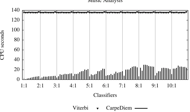
We measured the total classification time spent by the algorithms as well as the average time saved byCarpeDiemwith respect to the Viterbi algorithm. They are provided in Table 2: average time savings range from about 73% (FAQs segmentation) to over 96% (letter recognition). Fig-ures 4, 5 and 6 graphically report a detailed account of each experiment. Classification times for each problem were obtained using a fixed size test set. By observing the profiles reported in the fig-ures, it is apparent that, while the Viterbi algorithm runs in approximately constant time,CarpeDiem
performances depend on the particular classifier used.
0 20 40 60 80 100 120 140
1:1 2:1 3:1 4:1 5:1 6:1 7:1 8:1 9:1 10:1
CPU seconds
Classifiers Music Analysis
Viterbi CarpeDiem
Figure 4: Results on the music analysis problem. We report on the abscissas the learnt classifiers indicating i: j for classifier acquired using(10·i)% of the training set and j iterations. Labels on the abscissas refer only to the first classifier for each block of experiments; the following nine bars refer to the remaining ones. For instance, label 3:1 is positioned below the bar corresponding to the classifier trained on the 30% of the training set and using 1 iteration. The following nine bars refer to classifiers 3:2, 3:3,. . ., 3:10. We report on the ordinates the CPU seconds needed for the classification of the test set. Vertical bars refer to the time spent byCarpeDiem. Triangles refer to the time spent by Viterbi.
One interesting fact is unveiled by the profile of the classification time. Since—in each one of the three experiments—classification is performed on a data set of fixed size, one would expect roughly constant classification time. By converse, at least in the first two experiments (Figures 4 and 5), the emerging patterns are similar to those usually observed at learning time. We remark that the hundred runs of each experiment differ only in the set of weights used by the classifier. Then it is apparent that, as the voted perceptron learns, it somehow modifies the weights in a way that proves to be detrimental to the work ofCarpeDiem.
To explain the observed patterns, let us consider an informative vertical featureφ•and examine
the first iteration of the voted perceptron on a sequence of length T =100. Also, we assume that
φ• is asserted 60 times, and that it votes for the correct label 50 times out of 60. Even though
this example may seem unrealistic, it is not.6 The first iteration on the first sequence the voted
perceptron chooses labels at random. Then, the vast majority of them will be incorrectly assigned, thus implying a large number of feature weights updates. If all the labels for whichφ• is asserted
are actually mislabelled, due to the way the update rule acts, the weight associated to φ• will be
increased7by 40. This large increase occurs all at once at the end of the first iteration on the first sequence, and it is likely to overestimate the weight of φ•. The voted perceptron will spend the
rest of learning trying to compensate for this overestimation. However, subsequent updates will be
6. For instance, in the music analysis problem, this could be the case for the feature that votes for the chord that has exactly 3 notes asserted in the current event.
1 1.5 2 2.5 3 3.5 4 4.5 5 5.5
1:1 2:1 3:1 4:1 5:1 6:1 7:1 8:1 9:1 10:1
CPU seconds
Classifiers FAQs Segmentation
Viterbi CarpeDiem
Figure 5: Results on the FAQs Segmentation problem. The conventions adopted are the same as for Figure 4.
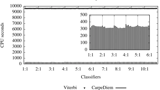
0 1000 2000 3000 4000 5000 6000 7000 8000 9000 10000
1:1 2:1 3:1 4:1 5:1 6:1 7:1 8:1 9:1 10:1
CPU seconds
Classifiers Letter Recognition
Viterbi CarpeDiem 0
100 200 300 400 500
1:1 2:1 3:1 4:1 5:1 6:1
Figure 6: Results on the letter recognition problem. In the inner frame we detail the time spent by
CarpeDiemusing the first fifty classifiers. The conventions adopted are the same as for Figure 4.
of smaller magnitude. In fact, the following predicted labeling will not be randomly guessed, thus implying a reduced number of updates.
-80 -60 -40 -20 0 20 40 60 80 100 120
0 7707 10708 13724 16755 19756 22772 25788 28804 31820
Weight
Number of updates
Number of updates
W
eigh
t
-80 -40
0
40 80
120
Figure 7: Evolution of vertical weights throughout learning. Each line corresponds to an individual vertical feature; vertical lines correspond to the beginning of new iterations. The plot refers to the music analysis data set.
learning steps of the voted perceptron where the time saved byCarpeDiemreaches peaks of 99.47% (music analysis, classifier 1:1) and 78.60% (FAQs segmentation, classifier 1:1).
Lastly, one might wonder why the observed pattern wasn’t seen in the text recognition problem. Notwithstanding that the problem itself is a sequential one, to model only bigrams probabilities proved—against our expectations—to be not enough to provide sufficient discrimination power to horizontal features. In other words, the horizontal features we devised contribute to the correct classification only in a marginal way. This is a setting whereCarpeDiemcan, and actually does, attain exceptional time savings (Figure 6).
Prompted by such time savings, we re-ran the same experiments using no horizontal features: the accuracy does not drop down as significantly as in the other two problems. This fact explains why the pattern observed in Figures 4 and 5 is not observed in Figure 6: since vertical features re-main predictive with respect to horizontal ones throughout the learning process the performances of
CarpeDiemdo not change over time. Here we note one important property ofCarpeDiem: Carpe-Diemtime performances reflect the degree of sequentiality inherent to the problem at hand. Actu-ally, by tracking the number of vertices opened in each layer, one can even measure how important sequential information is in different parts of the same sequence.
6.6 Comparison with Related Algorithms
6.6.1 RELATIONS WITHA∗
It could be argued that theCarpeDiemalgorithm looks interestingly similar to the A∗algorithm (Hart et al., 1968). In order to investigate this similarity let us consider the following heuristic, based on the same ideas underlyingCarpeDiem:
h(yt) =
∑
t′>t
max yt′
Sy0
t′
+S1∗
= (T−t)S1∗+
∑
t′>t
max yt′
S0y
t′
.
The heuristic estimates the distance to the goal by summing the best vertical weight in each layer and the best possible transition between any two layers.
Even though the heuristic is intuitively connected to the strategy implemented inCarpeDiem, the differences are indeed remarkable. A first important difference is in the choice criteria implemented in Algorithms 3 and 4 (we will focus only on Algorithm 3 for the sake of exposition). The criterion in Algorithm 3 states: do not consider any further node in this layer if
G(yt∗)>=Bt+S0
y′
t.
SinceBt=G(y∗
t−1) +S1∗, the above criterion approximates the reward of the optimal path by means
of S1∗only once rather than the T−t times taken by h(yt). Hence, A∗incurs an high risk of opening vertices in layers far from the goal only because of the cumulation of these approximations.
Another important difference between the two algorithms is in the fact that CarpeDiem imple-ments two different heuristics: one is used by Algorithm 3 and one is used by Algorithm 4. On the contrary A∗uses the same criterion throughout the computation. Finally, the data structures needed byCarpeDiemare simpler (and faster) than those needed to implement A∗.
In order to empirically assess whether A∗ could be competitive with respect toCarpeDiem, we implemented the above heuristic and paid particular attention to tuning the data structures. The resulting algorithm turned out to be even less efficient than the Viterbi algorithm.
Of course, this does not mean that the same principles implemented byCarpeDiemcould not be plugged into A∗by means of a carefully chosen heuristic. Rather, it shows that the problem is not trivial, and deserves ad-hoc research efforts.
6.6.2 VITERBIBEAMSEARCH
To compareCarpeDiemwith algorithms based on the Viterbi beam search (VBS) strategy presents several difficulties. On the one hand, we have an algorithm that guarantees optimality, but not com-putational performances; on the other hand, we have VBS approaches that guarantee comcom-putational performances abdicating optimality.
Let ξ be the ratio between the time spent by CarpeDiem and the time spent by the Viterbi algorithm for solving a given problem: that is, the time savings reported in Table 2 are computed as
[(1−ξ)×100]%. Given that the time spent by a Viterbi beam search algorithm is in the order of b2T , the time saved by a VBS algorithm w.r.t. the Viterbi algorithm is in the order of:
(K2−b2)T K2T =1−
b2 K2 .
By equating the time saved byCarpeDiem(i.e., 1−ξ) and the time saved via the VBS approach, we have that by setting:
b=pξK2 (8)
an algorithm based on the VBS approach will run in about the same time asCarpeDiem.
We implemented a basic VBS algorithm and measured its running time over the data set de-scribed in Section 6 and experimented with different settings of b. The results show that to obtain the same running times asCarpeDiem, the beam size needs to be set as follows:
• b=25 for the Tonal Harmony Analysis data set. Being K=78, this amounts to consider 32% of the possible labels;
• b=2 for the FAQ Segmentation data set. Being K=4, this amounts to consider 50% of the possible labels;
• b=5 for the text recognition data set. Being K =27, this amounts to consider 18.5% of the possible labels;
Two aspects are remarkable in the above results: i) the reported figures have been observed empir-ically rather than determined using the above formula. It is immediate to verify that they are very close to the ones returned by using Formula 8; ii) we omitted to implement a heuristic to guide the VBS search. Since computing the heuristic would require additional efforts, the timings used to derive such numbers are optimistic approximations of the actual time needed by a full fledged VBS algorithm.
In summary,CarpeDiemruns at least as fast as a VBS approach when a small to medium beam size is used while providing some additional benefits. Again, investigating the conditions that make appropriate one approach over the other one, deserves further deepening the research.
7. Conclusions
In this paper we have proposed CarpeDiem, a replacement of the Viterbi algorithm. On average,
CarpeDiem allows evaluating the best path in a layered and weighted graph in a fraction of the time needed by the Viterbi algorithm. CarpeDiem is based on a property exhibited by most tasks commonly tackled by means of sequential learning techniques: the observations at and around a time instant t are very relevant for determining the t-th label, while information about the succession of labels is mainly useful in order to disambiguate unclear cases. The extent to which the property holds determines the performances of the algorithm. We formally proved thatCarpeDiemfinds the best possible sequence of labels and that the algorithm complexity ranges between O(T K log K)in the best case, and O(T K2)in the worst case. The fact that the worst case complexity is the same as
In Section 3, we reviewed recently proposed alternatives and pointed out the following advan-tages ofCarpeDiemwith respect to the competitors:
• it is parameter free;
• it does not require any prior knowledge or tuning;
• it never compromises on optimality.
At the present time, the main strength of other approaches with respect to ours is that they have been devised to improve the forward-backward algorithm as well. We defer the extension of our approach in that direction to future work.
In addition to the theoretical grounding ofCarpeDiemcomplexity, we provided an experimen-tation on three real world problems, and compared its execution time with that of the Viterbi algo-rithm. The experiments show that large time savings can be obtained. The reported figures show time savings ranging from 73% to 96% with respect to the Viterbi algorithm.
A further interesting facet ofCarpeDiemis that its execution trace provides clues about the prob-lems at hand. It can then be used to understand how salient sequential information is. Also, within the same sequence, it is often interesting to investigate the time steps where sequential information gets crucial thus implying higher classification time. For instance, in Radicioni and Esposito (2007) we used this fact to find where musical excerpts get more difficult.
In a world where the quantity of information as well as its complexity is ever increasing, there is the need for sophisticated tools to analyse it in reasonable time. Our perception is that, in most problems, long chains of dependencies are useful to reach top results, but their influence on the correct labelling decreases with the length of the chain. In a probabilistic setting, the length of the chain of dependencies would be called the ‘order of the Markov assumption’. In such a context, it would be appropriate to say that what we call ‘vertical’ features are actually features making a zero order Markov assumption (no dependency at all), while horizontal features are features making a first order Markov assumption. The higher the order of the Markov assumption we want to plug into the model, the slower the algorithm that evaluates the sequential classifier. If our guess is correct, however, the higher the Markov assumption, the less informative are the features that use it. Should this be the case,CarpeDiemstrategy could be extended to efficiently handle higher order Markov assumptions, thereby allowing to use sequential classifiers to tackle a larger set of problems.
Acknowledgments
We wish to thank Luca Anselma, Guido Boella, Leonardo Lesmo, and Lorenza Saitta for their pre-cious advices on preliminary versions of the work. We also want to thank the anonymous reviewers for their helpful comments and suggestions.
Appendix A. Soundness
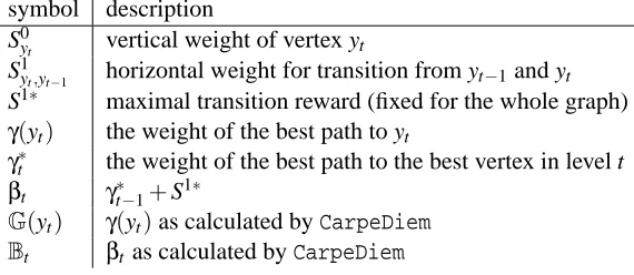
symbol description
S0yt vertical weight of vertex yt
S1yt,yt−1 horizontal weight for transition from yt−1and yt
S1∗ maximal transition reward (fixed for the whole graph)
γ(yt) the weight of the best path to yt
γ∗
t the weight of the best path to the best vertex in level t
βt γt∗−1+S1∗
G(yt) γ(yt)as calculated byCarpeDiem Bt βt as calculated byCarpeDiem
Table 3: Summary of the notation adopted.
keeping techniques can be used during the search to store path information. The path can be then be retrieved in O(T)time.
The proof consists in two Theorems and one Lemma; in particular, Theorem 1 directly im-plies the soundness ofCarpeDiem, while Theorem 2 and Lemma 1 are necessary in the proof of Theorem 1.
Before entering the core of the proof, let us summarize the notation adopted. We distinguish between values that are calculated byCarpeDiem, and those representing properties of the graph. We will use blackboard characters (GandB) to denote the former ones and greek letters (γandβ)
for the latter ones. A summary of important definitions is reported in Table 3.
We start by stating and proving Lemma 1, which ensures the soundness of the main bound used byCarpeDiem.
Lemma 1 IfBt=βt then the bound exploited by CarpeDiem does not underestimate the reward of
the optimal path to any vertex. Formally,
Bt =βt⇒Bt+S0y
t ≥γ(yt).
Proof Let us consider the optimal path to yt and denote withπ(yt)the predecessor of yt. Then, by definition we have:γt∗−1≥γ(π(yt)), and S1∗≥S1yt,π(yt). It immediately follows that:
γ∗
t−1+S1∗+Sy0t ≥γ(π(yt)) +S
1
yt,π(yt)+S
0
yt.
By definitionβt=γ∗t−1+S1∗andγ(yt) =γ(π(yt)) +S1yt,π(yt)+S0yt, which yields:
βt+S0yt ≥γ(yt)
and by assumption, this implies:
Bt+S0
yt ≥γ(yt).
Theorem 1 Let us consider a sequence of calls to Algorithm 3 on layers 2,3, . . . ,t(t≤T). When Algorithm 3 terminates on layer t, the returned vertex y∗t is the endpoint of the optimal path to layer t. Formally,
Proof We prove the stronger fact
Bt =βt∧ ∀yt :γ(y∗
t)≥γ(yt).
The proof is by induction on t. The base case for the induction is guaranteed by the initialization step in Algorithm 2 whereB2andγ(y∗
1)are set. We start by showing that
∀y1:γ(y1∗)≥γ(y1) (9)
as follows:
γ(y∗1) = γ(arg maxy1G(y1)) →by line 3 ( Algorithm 2) = γ arg maxy1S0y1 →by line 2 (Algorithm 2)
= γ(arg maxy1γ(y1)) →by Equation 2 = maxy1γ(y1)
⇓
∀y1:γ(y∗1)≥γ(y1).
In order to proveB2=β2, we note that Algorithm 2 setsB2toG(y∗ 1) +S1∗: B2= G(y∗
1) +S1∗ = S0y∗
1+S
1∗ →by line 2 (Algorithm 2) = γ(y∗1) +S1∗ →by Equation 2
= γ∗1+S1∗ →by definition ofγ∗1(Table 3) and Equation 9
= β2 →by definition ofβ2(Table 3).
Let us now assume that for all ˆt, 1≤ˆt<t:8
Bˆt=βˆt
∀yˆt:γ(y∗ˆt)≥γ(yˆt)
then we proveBt=βt as follows:
Bt= G(y∗
t−1) +S1∗ →by instruction 6 (Algorithm 3) = γ(y∗t−1) +S1∗ →by Theorem 2
= γt∗−1+S1∗ →by Equation 10 and definition ofγ∗t−1
= βt →by definition ofβt (Table 3).
In order to prove ∀yt :γ(yt∗)≥γ(yt) we start by noting that at the end of the main loop of Algorithm 3 it holdsG(y∗t)≥Bt+S0
y′t. Also, for any yt⊑ty
′
t we have (by Definition 2–Equation 5):
Bt+S0y
t ≤Bt+S
0
y′t. It follows that yt⊑ty
′
t ⇒G(y∗t)≥Bt+S0yt. Using Lemma 1 we have
yt ⊑t y′t⇒G(yt∗)≥γ(yt). (10)
8. We note that our definitions give no meaning toB1andβ1. We define them to be equal regardless their value: this