Integral Backstepping Control for a PMLSM Using Adaptive RNNUO

Integral Backstepping Control for a PMLSM Using Adaptive RNNUO

Chih-Hong Lin

1,*

, Chih-Peng Lin

2

1

Department of Electrical Engineering, National United University, Miaoli, Taiwan, ROC 2

Department of Engineering, Su-Mo Enterprise Co. LTD, Taichung, ROC

Received 17 July 2011; received in revised form 10 August 2011; accepted 17 September 2011

Abstract

Due to uncertainties exist in the applications of the a permanent magnet linear synchronous motor (PMLSM)

servo drive which seriously influence the control performance, thus, an integral backstepping control system using

adaptive recurrent neural network uncertainty observer (RNNUO) is proposed to increase the robustness of the

PMLSM drive. First, the field-oriented mechanism is applied to formulate the dynamic equation of the PMLSM

servo drive. Then, an integral backstepping approach is proposed to control the motion of PMLSM drive system.

With proposed integral backstepping control system, the mover position of the PMLSM drive possesses the

advantages of good transient control performance and robustness to uncertainties for the tracking of periodic

reference trajectories. Moreover, to further increase the robustness of the PMLSM drive, an adaptive RNN

uncertainty observer is proposed to estimate the required lumped uncertainty. The effectiveness of the proposed

control scheme is verified by experimental results.

Keywords: permanent magnet synchronous motor, recurrent neural network, integral backstepping control

1.

Introduction

The direct drive design of mechanical applications, which is based on PMLSM, has many advantages over its indirect

counterpart: such as no backlash and less friction, high speed and high precision in long distance location, simple mechanical

construction, high thrust force [1]. Therefore, the PMLSM is suitable for high-performance servo applications and has been

used widely for the industrial robots, semiconductor manufacturing systems, and machine tools, etc. [1-3].

The backstepping design provides a systematic framework for the design of tracking and regulation strategies suitable

for a large class of state feedback linearizable nonlinear systems. The approach can be extended to handle systems with

unknown parameters via adaptive backstepping [4-10]. The idea of backstepping design is to select recursively some

appropriate functions of state variables as pseudo-control inputs for lower dimension subsystems of the overall system. Each

backstepping stage results in a new pseudo-control design, express in terms of the pseudo control designs from preceding

design stages. When the procedure terminates, a feedback design for the true control input results achieves the original design

objective by virtue of a final Lyapunov function, which is formed by summing up the Lyapunov functions associated with each

individual design stage [4-10]. In addition, owing to the robust control performance of adaptive backstepping control and

sliding mode control, numerous combined adaptive backstepping and sliding-mode control schemes have appeared for both

*Corresponding author. E-mail address: [email protected]

linear and nonlinear systems [7-10].

The NNs can be mainly classified as feedforward neural networks (FNNs) and recurrent neural networks (RNNs)

according to the structures [11-18]. It is well known that an FNN is capable of approximating any continuous functions closely.

However, the FNN is a static mapping; it is unable to represent a dynamic mapping without the aid of tapped delays. The RNNs

[11-18] are a general case of artificial neural networks where the connections are not feed-forward ones only. In RNNs,

connections between units form directed cycles, providing an implicit internal memory. Those RNNs are adapted to problems

dealing with signals evolving through time. Their internal memory gives them the ability to naturally take time into account.

Valuable approximation results have been obtained for dynamical systems. The RNNs which comprise both feedforward and

feedback connections, have superior capabilities than FNNs, such as dynamic behavior and the ability to store information.

Since recurrent neuron has an internal feedback loop, it captures the dynamic response of a system without external feedback

through delays. Thus, RNNs are dynamic mapping and demonstrate good control performance in the presence of unmodelled

dynamics, parameter variations and external disturbances [11-18]. Lin et al. [17] incorporated recurrent neural network and an

adaptive backstepping controller to control linear induction motor drive for periodic reference trajectory tracking. Lin et al. [18]

developed adaptive backstepping controller and RNN uncertainty observer to control the periodic reference trajectory tracking

issue for a synchronous reluctance motor drive. For the purpose of real-time control, a RNN with simple network structure is

proposed in this study.

Due to uncertainties exist in the applications of the PMLSM servo drive which seriously influence the control

performance, thus, integral backstepping controller and adaptive RNNUO is proposed to control the rotor of the PMLSM to

track periodic references. In the proposed control scheme, an integral backstepping approach is proposed to control motion of

PMLSM drive system. Moreover, to further increase the robustness of the PMLSM drive, an adaptive RNNUO is proposed to

estimate the required lumped uncertainty in integral backstepping control system. Thus, an integral backstepping control

system using adaptive RNNUO is proposed to control the mover of the PMLSM to track periodic references. The effectiveness

of the proposed control scheme is verified by experimental results.

2.

Configuration of PMLSM Drive

The machine model of a PMLSM can be described in synchronous rotating reference frame as follows [1-3]:

d e q q s q Ri

v = +λ +ω λ (1)

q e d d s d Ri

v = +λ −ωλ (2)

where

q q q = Li

λ (3)

PM d d

d Li λ

λ = + (4)

r

e Pω

ω = ₍₅₎

and

v

d

,

v

q are the d and q axis voltages; are the d and q axis currents; Rsis the phase winding resistance; Ld,Lq are the

d and q axis inductances; ωr is the angular velocity of the mover;

ω

e is the electrical angular velocity;

λ

PM is the

permanent magnet flux linkage; P is the number of pole pairs. Moreover,

τ π

ωr= vr/ (6)

e r e Pν τ f

ν = =2 ₍₇₎

electromagnetic power is given by [2]

(

)

] /2 [

3 dq d q dq e

e e

e F P i L L ii

P = ν = λ + − ω (8)

Thus, the electromagnetic force is

(

)

τ

λ

π [ ]/2

3 d q d q dq

e P i L L ii

F = + − (9)

and the mover dynamic equation is

L r r

e Mv Dv F

F =  + + (10)

Where F_e is the electromagnetic force; M is the total mass of the moving element system; D _{is the viscous friction and} iron-loss coefficient; F_L is the external disturbance term.

The basic control approach of a PMLSM servo drive is based on field orientation [2]. The flux position in the d-q

coordinates can be determined by the Hall sensors. In (4), (8) and (9), ifid = 0, the d-axis flux linkage

λ

d is fixed since

PM

λ _{is constant for a PMLSM, and the electromagnetic force} Fe is then proportional to

*

q

i _{which is determined by}

closed-loop control. The rotor flux is produced in the d-axis only, while the current vector is generated in the q-axis for the

field-oriented control. Since the generated motor force is linearly proportional to the q-axis current as the d-axis rotor flux is

constant in (4), the maximum force per ampere can be achieved. The resulted force equation is

τ πλ /2 3 PMq

e i

F = (11)

The optimal electromagnetic performance for the actuator is therefore realized by controlling the primary current distributions

to lie in the q-axis, i.e., id =0

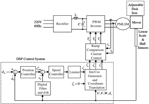
The configuration of a field-oriented PMLSM servo drive system is shown in Fig. 1, which consists of a PMLSM, a

ramp comparison current-controlled PWM VSI, a field-orientation mechanism, a coordinate translator, a speed control loop, a

position control loop, a linear scale and Hall sensors. The flux position of the PM is detected by the output signals of the Hall

sensors denoted U, V and W. Different sizes of iron disks can be mounted on the mover of PMLSM to change the mass of the

moving element and viscous friction. The field-oriented mechanism drive system was implemented by TMS320C32 DSP

control system. A host PC downloads the program running on the DSP. With the implementation of field-oriented control [1-3],

the PMLSM drive can be simplified to a control system with block diagram shown in Fig. 2, in which and this will yield a linear force per amp characteristic for the actuator.

*

q f e K i

F = (12)

τ λ

π /2

3 _PM

f P

K = ₍₁₃₎

D Ms s H_p

+

= 1

)

( ₍₁₄₎

where K_f is the thrust coefficient; i*q is the command of thrust current; s is the a Laplace's operator. The PMLSM used in this

study is 220V 3.5A 1kW 213N type. For the convenience of the controller design, the position and speed signals in the control

loop are set at 1V=0.075m and 1V=0.075m/sec. The parameters of the system are:

N/V 942 . 6 sec / kg 56 . 92

Nsec/V 2025 . 0 2.7kg

N/A, 8 . 60

= =

= =

=

D M K_f

(15)

Fig. 1 Configuration of DSP field-oriented control PMLSM drive system

Fig. 2 Simplified control system block diagram

3.

Integral Backstepping Control System Using Adaptive RNN Uncertainty Observer

Consider a drive system with parameter variations, external load disturbance, and friction force for the actual PMLSM

servo drive system, then (10) can be rewritten as

p r r v X

d = = (16)

L a A a a p a

p (A A)X (B B )U C F

X = +∆ + +∆ + (17)

r

d

Y = (18)

where d_r is the mover position of the PMLSM; Xp is the mover velocity of the

PMLSM;Aa =−D M ; Ba =Kf M >0; Ca =−1M ;

∆

A

and

∆

B

denote the uncertainties introduced by system

parameters M and D; U_A is the control input to the PMLSM drive system. Reformulate (17), then H

U B X A

Xp = a p + a A+ (19)

where H is named the lumped uncertainty and defined by

L A p BU CF

AX

H≡∆ +∆ + (20)

The lumped uncertainty H will be observed by an adaptive uncertainty observer and assumed to be a constant during the observation. The above assumption is valid in practical digital processing of the observer since the sampling period of the

observer is short enough to compare with the variation of H.

The control objective is to design an Integral backstepping control system for the output Y of the system shown in (18)

to track the reference trajectory Y_d(t), which is d_m, asymptotically. The proposed the Integral backstepping control system is designed to achieve the position-tracking objective and described step by step as follows.

b

T Tc 220V 60Hz Rectifier L C PWM Inverter Ramp Comparison Current Control Limiter Coordinate Translation Sin/Cos Generator and Digital Filter and d/dt + − 0 *₌ d i * q i * a i * b i * c i a T a i b i r d W V U, , ,

PMLSM ∗ r v ∑ + -∑ + -Position Controller Speed Controller m d r

d vr

Linear Scale & Hall Sensors Mover Adjustable Disk Iron

DSP Control System

b

T Tc 220V 60Hz Rectifier L C PWM Inverter Ramp Comparison Current Control Limiter Coordinate Translation Sin/Cos Generator and Digital Filter and d/dt + − 0 *₌ d i * q i * a i * b i * c i a T a i b i r d W V U, , ,

PMLSM ∗ r v ∑ + -∑ + -Position Controller Speed Controller m d r

d vr

Linear Scale & Hall Sensors Mover Adjustable Disk Iron

DSP Control System

∑

+ +

-PMLSM Drive System

*

q

i Fe

L F r v D Ms 1 + s 1 r d f K

( )s Hp Speed Controller * r v ∑ + -∑ + -Position Controller m d r v r d ∑∑ + +

-PMLSM Drive System

*

q

i Fe

L F r v D Ms 1 + s 1 r d f K

Step 1:

For the position-tracking objective, define the tracking error as

Y Y d d

z1= m− r = d − (21)

and its derivative is

p d d

1 Y Y Y X

z =  − =  − ₍₂₂₎

Define the following stabilizing function:

χ

α1=c1z1+Yd+c2 (23)

where

c

1and

c

2 are positive constants; χ =∫z1(τ)dτ is the integral action. We can ensure that tracking error converge to

zero by using integral action. Then, first Lyapunov function is chosen as

2 z

V 2

1

1 = / (24)

Define z2 =Xp−α1, then V₁ the derivative of is

χ

α 2 1

2 1 1 2 1 1 2 d 1 p d 1

1 z Y X z Y z z z cz c z

V = ( − )= ( − − )=− − − (25)

Step 2:

The derivative of

z

2 is now expressed as

1 p 2 X

z =  −α =AaXp +BaUA+H−c1z1−Yd −c2χ

(

2 α1

)

a A 1 1 d 2χ

a z BU H c z Y c

A + + + − − −

= _  (26)

To design the integral backstepping control system, the lumped uncertainty H is assumed to be bounded, i.e., H ≤H , and define the following Lyapunov function:

2 c 2 z V

V 2 2

2 2 1

2 = + / + χ / (27)

Using (25) and (26), the derivative of V2 can be derived as follows:

(

)

]

[ )

(

χ α

χ χ χ

χ χ

2 d 1 1 A

a 1 2 a 2 2 1 2 2 1 1 2 1

2 2 2 1 2 1 2

c Y z c H U B z

A z c z c z c z z

c z z V z , z V

− − − + + + +

+ − − − =

+ + =

   

   

[

_{1 a}( ₂ α₁) _{a A}

]

₂[ _{1 1 d 2}χ]

2 2 1

1z z z A z BU H z c z Y c

c + − + + + + − + +

−

= _ 

(28)

According to (28), an integral backstepping control law

U

A is designed as follows:

] )

( )

(

[ 1 2 2 a 2 α1 2 1 1 d 2χ

1 a

A B z c z A z Hsgn z c z Y c

U = − − − + − +  + + (29)

where c1 and c2

) (

)

(z ,z c z c z z H z H c z c z z H H

V_{2 1 2} =− _{1 1}2− _{2 2}2+ ₂ − ₂ ≤− _{1 1}2− _{2 2}2− ₂ −

are positive constants. Substitute (29) into (28), the following equation can be obtained:

2 2 2 2 1

1z c z

c −

−

≤ (30)

) ( )

( 2 1 2

2 2 2 2 1

1z c z V z ,z

c

t = + ≤−

Θ (31)

Then

∫tΘ _d ≤_{V z z} −_{V z t z t}

0 (τ) τ 2(1(0), 2(0)) 2( 1(), 2()) (32)

SinceV₂(z₁(0),z₂(0)) is bounded, and V₂(z₁(t),z₂(t)) is non-increasing and bounded, then_tlim_→∞∫0tΘ(τ)dτ<∞

( )

t

Θ

. Moreover,

is bounded, then and Θ

( )

t is uniformly continuous [19]. By using Barbalat’s lemma [19], it can be shown that tlim→∞Θ(t)=0. That is

z

1 and

z

2will converge to zero as

t

→

∞

. Moreover, tlim→∞Y(t)=Ydand tlimXp Yd



=

∞

→ . Therefore, the

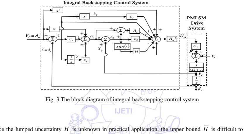
integral backstepping control system is asymptotically stable. The stability of the proposed the integral backstepping control

system, which is shown in Fig. 3, can be guaranteed.

Fig. 3 The block diagram of integral backstepping control system

Step 3:

Since the lumped uncertainty H is unknown in practical application, the upper bound H is difficult to determine. Therefore, a RNN uncertainty observer is proposed to adapt the value of the lumped uncertainty Hˆ . A three-layer RNN,

which comprises an input (the i layer), a hidden (the j layer) and an output layer (the k layer), is adopted to implement the

proposed control system. The signal propagation and the activation function in each layer is introduced as follows:

Layer 1: Input Layer

( )

( )

( )

(

( )

)

_{( )} i 12 e 1 1 N net f N y N x N net N net 1 i 1 i 1 i 1 i 1 i 1 i , , , = + = =

= ₋ (33)

where

x

1i represents the ith input to the node of input layer; N denotes the number of iterations;

1

i

f

is the activation function,

which is a sigmoidal function. The inputs of the RNN are the tracking errorem, which is the difference between the output of

the reference model

d

_m and the mover position

d

_r, and its derivative.

Layer 2: Hidden Layer

( )

=

(

−

)

+∑

( )

, i 2 i 2 ij 2 j 2 j 2

j N w y N 1 w x N

net

( )

(

( )

)

( ) j 12 l

e 1 1 N net f N y N net 2 j 2 j 2 j 2 j ..., , , , = + =

= ₋ (34)

where w2j are the recurrent weight for the units in the hidden layer;

2

ij

w are the connective weights between the input layer and the hidden layer; l is the number of neurons in the hidden layer; fj2 is the activation function, which is also a sigmoidal

function; y_i1(N)=x_i2(N) _{represents the jth input to the node of hidden layer.} 1 c s 2 z 1 z 1 α -+ p X r d Y= m d d Y = 2 s 1 a B− f K e F r v r d s 1 PMLSM Drive System L F D Ms 1 + A U Σ Σ Σ Σ Σ + -+

s z1

a A 2 c 1 c -+ -+ Integral Backstepping Control System

-s 1 2 c χ + + Σ + + ₊ H + + ( )⋅ sgn 1 c s 2 z 1 z 1 α -+ p X r d Y= m d d Y = 2 s2 s 1 a B− f K e F r v r d s 1 PMLSM Drive System L F D Ms 1 + A U Σ Σ Σ Σ Σ Σ Σ

Σ ΣΣ

+

-+

s z1

a Aa A 2 c 1 c -+ -+ Integral Backstepping Control System

Layer 3: Output Layer

( )

N w x

( )

N y

( )

N f

(

net

( )

N

)

net k 1

net k3

3 k 3 k 3 k j 3 j 3 jk 3

k =∑ , = = , = (35)

where w3jk are the connective weights between the hidden layer and the output layer;

3

k

f is the activation function, which is

set to be unit; y (N) x3j(N) 2

j = represents the kth input to the node of output layer. The output of the RNN U y3(N) k

R = is

rewritten as follows:

Γ Ο

Ο T

R H

U = ˆ( )= (36)

where

[

3

]

T

1 l 3 21 3

11 w w

w 

=

Ο is the collections of the adjustable parameters of RNN.

[

x x xl

]

T

3 3 2 3 1 

=

Γ , in which x3j is

determined by the selected sigmoidal function and 0≤ 3≤1

j

x .

To develop the adaptation laws of the RNN uncertainty observer, the minimum reconstructed error E is defined as follows:

) (Ο*

H H

E= − (37)

where Ο* is an optimal weight vector that achieves the minimum reconstructed error, and the absolute value of E is assumed to be less than a small positive constant, E (i.e., E ≤E). Then, a Lyapunov candidate is chosen as

) ( ) ( 2 1 ) ˆ ( 2

1 2 * *

2

3=V + E−E + Ο−Ο T Ο−Ο

V

η

ρ (38)

where

ρ

and

η

are positive constants;

E

ˆ

is the estimated value of the minimum reconstructed error E. The estimation of the reconstructed error E is to compensate the observed error which is induced by the RNN uncertainty observer and to

further guarantee the stable characteristic of the whole control system. Take the derivative of the Lyapunov function from Eq.

(38)

[

z A z BU H

]

z z c 1 E E E 1 V V A a 1 2 a 1 2 2 1 1 T 2 3 + + + + − + − = − + − + = ) ( ) ( ˆ ) ˆ ( * α η

ρ Ο Ο Ο

   Ο Ο Ο      T 2 d 1 1 2 1 E E E 1 c Y z c

z[ _{+ +} ]₊ (ˆ₋ )ˆ₊ ( ₋ *) −

η ρ

χ

(39)

According to (39), an integral backstepping control with adaptive law U_A =Uˆ_A is proposed as follows:

)] ( ˆ ˆ ) ( [

ˆ _{α χ}

2 d 1 1 1 2 a 2 2 1 1 a A

A U B z c z A z E H c z Y c

U = = − − − + − − +  + + (40)

Substituting (40) into (39), the following equation can be obtained

Ο Ο Ο    T 2 2 2 2 2 2 2 1 1 3 1 E E E 1 E z H z H z z c z c

V =− − + − ˆ − ˆ+ (ˆ− )ˆ + ( − *) η ρ Ο Ο Ο Ο Ο

Ο  T 

2 2 2 2 2 2 2 1 1 1 E E E 1 H H z H H z E z z c z

c _{− −} ˆ₊ ( ₋ ˆ( *))₊ (ˆ( *)₋ ˆ( ))₊ (ˆ₋ )ˆ₊ ( ₋ *) − = η ρ Ο Ο Ο Γ Ο

Ο T  T 

2 2 2 2 2 2 1 1 1 E E E 1 z E E z z c z

c _{− −} (ˆ₋ )₋ ( ₋ *) ₊ (ˆ₋ )ˆ₊ ( ₋ *) −

=

η ρ

(41)

The adaptation laws for Ο and

E



ˆ

are designed as follows:

Γ

2

ˆ _z

E=ρ ₍₄₃₎

Thus, (32) can be rewritten as follows:

0 t z c z c

V 2 22

2 1 1

3 =− − =Θ()≤

 (44)

By using Barbalat’s lemma [19], it can be shown that Θ(t)→0 as t→∞, that is,

z

1 and

z

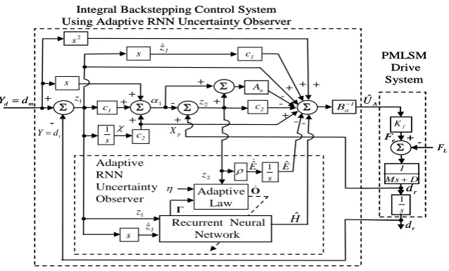
2will converge to zero as t→∞. As a result, the stability of the proposed integral backstepping control system by using an adaptive RNNUO, which is shown

in Fig. 4, can be guaranteed. On the other hand, the guaranteed convergence of tracking error to be zero does not imply

convergence of the estimated value of the lumped uncertainty to it real values. The persistent excitation condition [19] should

be satisfied for the estimated value to converge to its theoretic value.

In order to train the RNN effectively, an on-line parameter training methodology can be derived by using adaptation

laws Ο of above the Lyapunov stability theorem. Then adaptation laws of the parameters in the RNN, (w w w2j ) 2 ij 3 jk, , Ο 3 j R 3 3 jk 3 k 3 k 3 k 3 k R R 3 2 3 jo x U V w net net y y U U V z w ∂ ∂ η ∂ ∂ ∂ ∂ ∂ ∂ ∂ ∂ η

η ∆− =−

= Γ



,

can be computed by using the gradient descent method and the backpropagation algorithm as follows:

(45)

The above Jacobian term of controlled system can be rewritten as ∂V₃ ∂U_R =−z₂ . The error term can be calculated as

2 3 k R R 3 k z y U U V = − ∆ ∂ ∂ ∂ ∂ δ (46)

The recurrent weight of hidden layer 2 j

w can be updated as

j 3 jk k 2 j 2 j 2 j 3 k 3 k 3 k 3 k R R 3 2 j 3 2

j w P

w y y net net y y U U V w V w δ ∂ ∂ ∂ ∂ ∂ ∂ ∂ ∂ ∂ ∂ ∂ ∂ _{=− =} − ≡  (47) where 2 j 2 j

j y w

P ≡∂ ∂ can be calculated from (34). The weight between hidden layer and input layer can be updated as

ji 3 jk k 2 ji 2 j 2 j 3 k 3 k R R 3 ji 3 2

ji w Q

w y y y y U U V w V w δ ∂ ∂ ∂ ∂ ∂ ∂ ∂ ∂ ∂ ∂ _{=− =} − ≡ (48) where 2 ji 2 j

ji y w

Q ≡∂ ∂ can be calculated from (34).

Fig. 4 The block diagram of integral backstepping control system using adaptive RNNUO ρ

s

1 Eˆ

Adaptive Law

s

Recurrent Neural Network η Γ 2 z Ο 1 z  1 z Hˆ Adaptive RNN Uncertainty Observer

Eˆ

1 c s 2 z 1 z 1 α -+ p X r d Y= m d d Y = 2 s 1 a B− f K e F r d r d s 1 PMLSM Drive System L F D Ms 1 + A Uˆ Σ Σ Σ Σ Σ + -+

s z1

a A 2 c 1 c -+ -+ -+ + Σ + + ₊ + + - -s 1 2 c χ

Integral Backstepping Control System Using Adaptive RNN Uncertainty Observer

ρ

s

1 Eˆ

Adaptive Law

s

Recurrent Neural Network η Γ 2 z Ο 1 z  1 z Hˆ Adaptive RNN Uncertainty Observer

Eˆ

1 c s 2 z 1 z 1 α -+ p X r d Y= m d d Y = 2 s2 s 1 a B− f K e F r d r d s 1 PMLSM Drive System L F D Ms 1 + A Uˆ Σ Σ Σ Σ Σ Σ Σ

Σ ΣΣ

+

-+

s z1

a Aa A 2 c 1 c -+ -+ -+ + Σ Σ + + ₊ + + - -s 1 2 c χ

4.

Experimental Results

A block diagram of the DSP control system for a PMLSM drive is depicted in Fig. 1. A host PC downloads the program

running on the DSP. The proposed controllers are implemented by DSP control system. The current-controlled PWM VSI is

implemented by the IGBT power modules with a switching frequency of 15kHz. A DSP control board includes multi-channels

of D/A and encoder interface circuits. The coordinate transformation in the field-oriented mechanism is implemented by DSP

control system.

The parameters of the proposed adaptive integral backstepping control system by using RNNUO are given in the

following:

2

c1= , c2=1, ρ=0.2 (49)

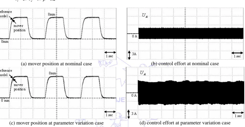
(a) mover position at nominal case (b) control effort at nominal case

(c) mover position at parameter variation case (d) control effort at parameter variation case

Fig. 5 Experimental results of the integral backstepping control system due to periodic step command.

All the gains in the integral backstepping control system without adaptive RNNUO and with adaptive RNN uncertainty

observer are chosen to achieve the best transient control performance in experimentation considering the requirement of

stability. The learning rate of adaptation laws of the parameters in the adaptive RNN uncertainty observer is set to

η

=0.1.

The node numbers of adaptive RNNUO have three, thirty and one neurons at the input, hidden and output layers, respectively.

Usually, some heuristics can be used to roughly initialize the parameters of the adaptive RNNUO for practical applications in

the experimental results. The control objective is to control the mover to move 8mm periodically. Then, when the command is

a sinusoidal reference trajectory, the reference model is set to be unit gain. The sampling interval of the control processing in

the experimentation is set at 1msec. Some experimental results are provided to demonstrate the control performance of the

proposed control systems. Two test conditions are provided in the experimentation, which are the nominal case and the

parameter variation case. The parameter variation case is the addition of one iron disk with 8.1kg weight to the mass of the

mover, i.e., the total mass is 3 times the nominal mass. First, the experimental results of the integral backstepping control

system for a periodic step and sinusoidal command at the nominal condition and the parameter variation condition are depicted

in Figs. 5 and 6. The position responses of the mover due to a periodic step command at the nominal condition and parameter

variation condition are depicted in Fig. 5(a) and 5(c); the associated control efforts are depicted in Fig. 5(b) and 5(d). The

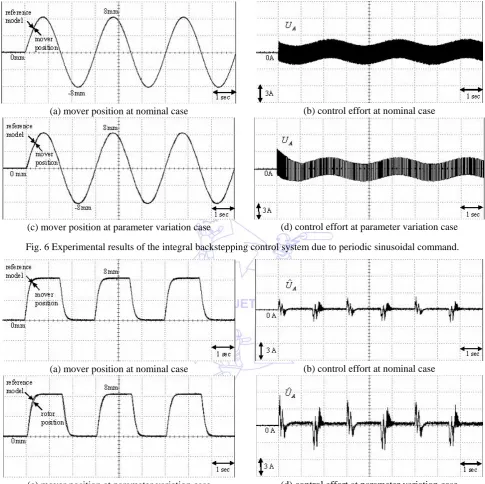
6. The position responses of the mover at the nominal case and the parameter variation case are shown in Figs. 6(a), and 6(c);

the associated control efforts are shown in Figs. 6(b) and 6(d). Though favorable tracking responses can be obtained by the

integral backstepping control system, the chattering phenomena in the control efforts are serious due to large control gain.

Moreover, the chattering control efforts will wear the bearing mechanism and might excite unstable system dynamics.

(a) mover position at nominal case (b) control effort at nominal case

(c) mover position at parameter variation case (d) control effort at parameter variation case

Fig. 6 Experimental results of the integral backstepping control system due to periodic sinusoidal command.

(a) mover position at nominal case (b) control effort at nominal case

(c) mover position at parameter variation case (d) control effort at parameter variation case

Fig. 7 Experimental results of the integral backstepping control system using an adaptive RNNUO due to periodic step command.

The experimental results of the integral backstepping control system by using an adaptive RNN uncertainty observer for a

periodic step and sinusoidal command at the nominal condition and the parameter variation condition are depicted in Figs. 7

and 8. The position responses of the mover due to a periodic step command at the nominal condition and parameter variation

condition are depicted in Fig. 7(a) and 7(c); the associated control efforts are depicted in Fig. 7(b) and 7(d). The tracking

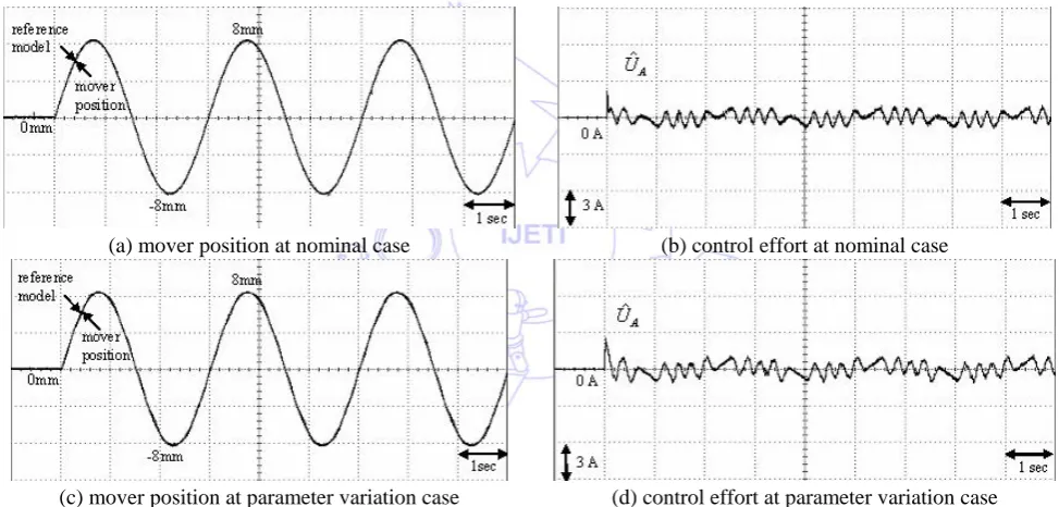
responses due to a periodic sinusoidal command at the nominal case and the parameter variation case are shown in Fig. 8. The

position responses of the mover at the nominal case and the parameter variation case are shown in Figs. 8(a), and 8(c); the

to periodic sinusoidal command at the nominal condition and parameter variation condition shown in Figs. 6(a), 6(c), 8(a), and

8(c) are relatively smoother due to periodic step command at the nominal condition and parameter variation condition shown

in Figs. 5(a), 5(c), 7(a), and 7(c), thus, the amplitude of the associated control efforts of the mover for a PMLSM due to

periodic sinusoidal command at the nominal condition and parameter variation condition shown in Figs. 6(b), 6(d), 8(b), and

8(d) are more relaxed due to periodic step command at the nominal condition and parameter variation condition shown in Figs.

5(b), 5(d), 7(b), and 7(d). Another friction forces and mass variation responses due to periodic sinusoidal command at the

nominal condition and parameter variation condition are more relaxed due to periodic step command at the nominal condition

and parameter variation condition. Since all the parameters of the RNN are initialized by using the pre-trained data, accurate

tracking control performance of the PMLSM servo drive can be obtained in the first cycle. Moreover, the chattering is much

reduced in the control efforts of the integral backstepping control system by using an adaptive RNN uncertainty observer as

shown in Figs. 7(b), 7(d), 8(b) and 8(d). However, the robust control performance of the proposed integral backstepping

control system using an adaptive RNN uncertainty observer under the occurrence of parameter variations at different

trajectories are obvious owing to the on-line adaptive adjustment of the RNN uncertainty observer. From the experimental

results, the control performance of the proposed integral backstepping control system by using an adaptive RNNUO is better

than the integral backstepping control system for the tracking of periodic commands.

(a) mover position at nominal case (b) control effort at nominal case

(c) mover position at parameter variation case (d) control effort at parameter variation case

Fig. 8 Experimental results of the integral backstepping control system by using an adaptive RNNUO due to periodic sinusoidal command.

5.

Conclusions

An integralbackstepping control system using adaptive recurrent neural network uncertainty observer (RNNUO) is

proposed to control PMLSM drive for the tracking of periodic reference inputs. First, the field-oriented mechanism is applied

to formulate the dynamic equation of the PMLSM servo drive. Then, an integralbackstepping control system using adaptive

RNNUO is developed to control PMLSM drive under the occurrence of parameter variations. With the proposed integral

backstepping control system, the mover position of the PMLSM drive possesses the advantages of good transient control

performance and robustness to uncertainties for the tracking of periodic reference trajectories. Moreover, to further increase

the robustness of the PMLSM drive, an adaptive RNN uncertainty observer is proposed to estimate the required lumped

6.

Acknowledgements

The author would like to acknowledge the financial support of the National Science Council in Taiwan, R.O.C. through

its grant NSC 99-2221-E-239-040-MY3.

References

[1] I. Boldea and S. A. Nasar, Linear electric actuators and generators, London, Cambridge University Press, 1997. [2] T. Egami, and T. Tsuchiya, “Disturbance suppression control with preview action of linear DC brushless motor,” IEEE

Trans. Ind. Electron., vol. 42, pp. 494-500, Oct.1995.

[3] M. Sanada, S. Morimoto, and Y. Takeda, “Interior permanent magnet linear synchronous motor for high-performance drives,” IEEE Tran. Ind. Appl., vol. 33, pp. 966-972, July/Aug. 1997.

[4] M. Krstic and P. V. Kokotovic, “Adaptive nonlinear design with controller-identifier separation and swapping,” IEEE Trans. Automat. Contr., vol. 40, pp. 426-440, March 1995.

[5] M. Krstic, I. Kanellakopoulos, and P. V. Kokotovic, Nonlinear and adaptive control design. New York: Wiley, 1995. [6] A. Stotsky, J. K. Hedrick, and P. P. Yip, “The use of sliding modes to simplify the backstepping control method,” Proc. of

American Control Conf., pp. 1703–1708, June 1997.

[7] G. Bartolini, A. Ferrara, L. Giacomini, and E. Usai, “Properties of a combined adaptive/second-order sliding mode control algorithm for some classes of uncertain nonlinear systems,” IEEE Trans. Automat. Contr., vol. 45, pp. 1334–1341, July 2000.

[8] F. J. Lin, P. H. Shen, and S. P. Hsu, “Adaptive backstepping sliding mode control for linear induction motor drive,” IEE Proc., Electr. Power Appl., vol. 149, pp. 184–194, May 2002.

[9] C. C. Wang, N. S. Pai, H, T. Yau, “Chaos control in AFM system using sliding mode control by backstepping design, ” Communications in Nonlinear Science and Numerical Simulation, vol. 15, pp. 741-751, 2010.

[10]C. L. Chen, C. C. Peng and H. T. Yau, “High-order sliding mode controller with backstepping design for aeroelastic systems,” Communications in Nonlinear Science and Numerical Simulation, vol. 17, pp.1813-1823, 2012.

[11]T. W. S. Chow and Y. Fang, “A recurrent neural-network-based real-time learning control strategy applying to nonlinear systems with unknown dynamics,” IEEE Trans. Ind. Electron., vol. 45, pp. 151-161, Feb. 1998.

[12]S.C. Sivakumar, W. Robertson, and W. J. Phillips, “On-line stabilization of block-diagonal recurrent neural networks,” IEEE Trans. Neural Networks, vol. 10, pp. 167-175, Jan. 1999.

[13]M. A. Brdys and G. J. Kulawski, “Dynamic neural controllers for induction motor,” IEEE Trans. Neural Networks, vol. 10, pp. 340-355, March 1999.

[14]H. Cardot, Recurrent neural networks for temporal data processing, InTech,Open Access Publisher, 2011.

[15]J. Martens and I. Sutskever, “Learning recurrent neural networks with Hessian-free optimization,” in Proceedings of the28th

[16]Q. Liu and J. Wang, “Finite-time convergent recurrent neural network with a hard-limiting activation function for constrained optimization with piecewise-linear objective functions,” IEEE Trans. Neural Networks, vol. 22, pp. 601-613, April 2011.

International Conference on Machine Learning, Bellevue, Washington, USA, 2011.

[17]F. J. Lin, R. J. Wai, W. D. Chou and S. P. Hsu, “Adaptive backstepping control using recurrent neural network for linear induction motor drive,” IEEE Trans. Ind. Electron., vol. 49, pp.134-146, Feb. 2002.

[18]C. H. Lin, A. J. Chen and Y. S. Tsai, “Adaptive backstepping control for synchronous reluctance motor drive using RNN uncertainty observer,” IEEE Power Electronics Specialists Conf., pp. 542-547, Orlando, FL., June 2007.